A&A 379, 1052-1082 (2001) 105220011320
J. M. Krijger1 - R. J. Rutten1 - B. W. Lites2 - Th. Straus3 - R. A. Shine4 - T. D. Tarbell4
1 - Sterrekundig Instituut,
Postbus 80000,
3508 TA Utrecht,
The Netherlands
2 -
High Altitude Observatory,
National Center for Atmospheric Research,
PO Box 3000,
Boulder CO 80307-3000,
USA
3 -
Osservatorio Astronomico di Capodimonte,
Via Moiariello 16,
80131 Napoli,
Italy
4 -
Lockheed Martin Solar and Astrophysics Lab,
Dept. L9-41, Building 252, 3251 Hanover Street,
Palo Alto,
CA 94304,
USA
Received 13 June 2001 / Accepted 14 September 2001
Abstract
We analyze oscillations in the solar atmosphere using image
sequences from the Transition Region and Coronal Explorer
(TRACE) in three ultraviolet passbands which sample the upper solar
photosphere and low chromosphere.
We exploit the absence of atmospheric seeing in TRACE data to
furnish comprehensive Fourier diagnostics (amplitude maps,
phase-difference spectra, spatio-temporal decomposition) for
quiet-Sun network and internetwork areas with excellent sampling
statistics.
Comparison displays from the ground-based Ca IIH spectrometry that
was numerically reproduced by Carlsson & Stein are added to link
our results to the acoustic shock dynamics in this simulation.
The TRACE image sequences confirm the dichotomy in oscillatory
behaviour between network and internetwork and show upward
propagation above the cutoff frequency, the onset of acoustic shock
formation in the upper photosphere, phase-difference contrast
between pseudo-mode ridges and the interridge background, enhanced
three-minute modulation aureoles around network patches, a
persistent low-intensity background pattern largely made up of
internal gravity waves, ubiquitous magnetic flashers, and low-lying
magnetic canopies with much low-frequency modulation.
The spatio-temporal occurrence pattern of internetwork grains is
found to be dominated by acoustic and gravity wave interference.
We find no sign of the high-frequency sound waves that have been
proposed to heat the quiet chromosphere, but such measurement is
hampered by non-simultaneous imaging in different passbands.
We also find no signature of particular low-frequency fluxtube waves
that have been proposed to heat the network.
However, internal gravity waves may play a role in their excitation.
Key words: Sun: photosphere - Sun: chromosphere - Sun: oscillations
This paper addresses oscillations of the quiet solar atmosphere from
image sequences taken with the Transition Region and Coronal
Explorer (TRACE).
TRACE images the Sun from a Sun-synchronous orbit at characteristic
temperatures between 104K and 107K by sequentially
selecting different spectral passbands to feed a
![]() px2 CCD camera with 0.5 arcsec pixels (366 km/px on the
Sun) that covers nearly 10% of the solar disk.
Details are given by Handy et al. (1999).
First results from the spectacular coronal movies taken through the
TRACE far-ultraviolet passbands were presented by
Schrijver et al. (1999).
px2 CCD camera with 0.5 arcsec pixels (366 km/px on the
Sun) that covers nearly 10% of the solar disk.
Details are given by Handy et al. (1999).
First results from the spectacular coronal movies taken through the
TRACE far-ultraviolet passbands were presented by
Schrijver et al. (1999).
In this paper we use image sequences taken through the
ultraviolet TRACE passbands centered at
![]() ,
1600, and
1550Å to study quiet-Sun oscillations in the upper photosphere
and low chromosphere.
We so return to the domain of the pioneering rocket studies of
1600Å "cell grains'' by Brueckner (1980) and
Cook et al. (1983) using the HRTS rocket
spectrograph, and by Bonnet et al. (1982), Foing & Bonnet
(1984a,b), Foing et al. (1986), and
Damé et al. (1986) using the TRC rocket filtergraph.
The obvious improvement that TRACE brings over the TRC flights is
enormous sequence duration increase and digital data registration
per CCD instead of emulsion.
TRACE has no spectrograph so that emulation of the HRTS flights
requires multi-spacecraft campaigns as in the recent
TRACE-plus-SUMER (and MDI) analysis of
Judge et al. (2001).
The strength of the present analysis is the large
statistical significance offered by TRACE image sequences and the
use of comprehensive and complementary Fourier diagnostics to
provide a complete inventory.
,
1600, and
1550Å to study quiet-Sun oscillations in the upper photosphere
and low chromosphere.
We so return to the domain of the pioneering rocket studies of
1600Å "cell grains'' by Brueckner (1980) and
Cook et al. (1983) using the HRTS rocket
spectrograph, and by Bonnet et al. (1982), Foing & Bonnet
(1984a,b), Foing et al. (1986), and
Damé et al. (1986) using the TRC rocket filtergraph.
The obvious improvement that TRACE brings over the TRC flights is
enormous sequence duration increase and digital data registration
per CCD instead of emulsion.
TRACE has no spectrograph so that emulation of the HRTS flights
requires multi-spacecraft campaigns as in the recent
TRACE-plus-SUMER (and MDI) analysis of
Judge et al. (2001).
The strength of the present analysis is the large
statistical significance offered by TRACE image sequences and the
use of comprehensive and complementary Fourier diagnostics to
provide a complete inventory.
In standard models of the solar atmosphere such as VAL-C of
Vernazza et al. (1973, 1976, 1981)
and FAL-C of
Fontenla et al. (1993), the disk-center intensity at
1700Å emerges from the "upper photosphere'', 1550Å radiation from the "lower chromosphere'', and 1600Å radiation
from the "temperature minimum region'', where the temperature
minimum at h = 500km above continuum optical depth
![]() at
at
![]() Å defines the transition
from photosphere to chromosphere (see the formation panels in
Fig. 36 of Vernazza et al. 1981).
The ubiquitous existence of a chromospheric temperature rise in
shell-like ("plane-parallel'') stratification over
h = 500 - 1000km is presently in debate on the basis of the very
oscillations discussed here and reviewed below, but we maintain
this nomenclature for clarity.
Also, we prefer to use "chromospheric dynamics'' even for the
upper-photosphere diagnostics since the TRACE UV passbands
essentially sample the onset of chromospheric oscillations and the
chromospheric network.
Å defines the transition
from photosphere to chromosphere (see the formation panels in
Fig. 36 of Vernazza et al. 1981).
The ubiquitous existence of a chromospheric temperature rise in
shell-like ("plane-parallel'') stratification over
h = 500 - 1000km is presently in debate on the basis of the very
oscillations discussed here and reviewed below, but we maintain
this nomenclature for clarity.
Also, we prefer to use "chromospheric dynamics'' even for the
upper-photosphere diagnostics since the TRACE UV passbands
essentially sample the onset of chromospheric oscillations and the
chromospheric network.
The same atmospheric regime is accessible to ground-based observation and has been studied extensively using the cores of strong absorption lines and the Ca II K2V and H2V inner-wing reversals. Although TRACE does not reach the angular resolution of ground-based telescopes at good seeing, TRACE image sequences offer the important advantage of distortion-free sampling over relatively long duration. Compared with oscillation studies employing Fraunhofer line spectrometry in the visible to probe these and lower heights in the solar atmosphere or ultraviolet line spectrometry to probe greater heights, the lack of Dopplershift information is a disadvantage, but TRACE imaging yields data from a far larger area than is sampled by a spectrograph slit and so permits a much more complete view of solar variations as well as much better statistical reliability in their diagnosis. In addition, the wide-band continua sampled by the TRACE 1700 and 1600Å passbands do not suffer Dopplershift contamination as is the case for the apparent brightness modulation of optically thick lines (including the inner wings of Ca IIH & K, see Sect. 4.3). These outstanding TRACE capabilities are exploited here to wrap up much previous work.
The extensive older literature on oscillations in the upper
photosphere and lower chromosphere has been reviewed by
Rutten & Uitenbroek (1991a); more recent work is reviewed by
Rutten (1994, 1995, 1999, 2001).
Stein & Carlsson (1997), Carlsson & Stein (1998),
Carlsson (1999), Deubner (1998), and
Deubner & Steffens (1999).
Even in quiet-Sun areas strict distinction must be made between
network and internetwork.
The first term denotes those parts of the supergranular cell
boundaries that contain kiloGauss magnetic elements at sufficient
spatial density to show up on photospheric magnetograms and on
chromospheric images taken in the core of Ca IIK or the
ultraviolet TRACE passbands.
On such filtergrams the chromospheric network appears as chains of
bright patches, each corresponding to a cluster of thin magnetic
elements in the underlying photosphere.
The latter, commonly identified with the modeller's fluxtubes, make
up the magnetic network and may appear as individual bright grains
in high-resolution (better than 0.5 arcsec) movies made in the
Fraunhofer G band around
![]() Å (e.g.,
Muller et al. 1989; Title & Berger 1996;
Berger et al. 1998; movies on the Dutch Open Telescope
website (URL http://dot.astro.uu.nl).
Å (e.g.,
Muller et al. 1989; Title & Berger 1996;
Berger et al. 1998; movies on the Dutch Open Telescope
website (URL http://dot.astro.uu.nl).
The bright patches on chromospheric filtergrams map the supergranular cell boundaries too sparsely to make the network identifiable as cellular patterning on snapshot images (cf. Hagenaar et al. 1997), but they stand out in longer-duration image sequences by being generally brighter and much more stably present than the transient, often briefly repetitive and often fast-moving, grainy brightness features seen in the intervening "internetwork'' areas corresponding to supergranular cell interiors.
The high degree of cospatiality of the brightness features seen in Ca IIK and the TRACE ultraviolet channels has been demonstrated by Rutten et al. (1999a). The correspondence between network grains in Ca IIK and clusters of smaller G-band magnetic elements located in underlying intergranular lanes is illustrated in Fig. 2 of Lites et al. (1999). The dynamical behaviour of the Ca IIK internetwork brightness patterning is illustrated in Fig. 3 of the same paper. Figure 5 of Rutten et al. (1999b) illustrates similar behaviour in a TRACE 1550Å image sequence. Figure 5 below shows a comparable 1700Å sequence.
The internetwork "three-minute'' oscillations (often in their
"internetwork grain'' disguise and often called "K2V grains'', see Rutten & Uitenbroek 1991a) are intensely
discussed in the recent literature after their identification as
weak acoustic shocks by Carlsson & Stein (1992, 1994, 1995, 1997,
1998).
Major issues that are presently in
debate are, respectively: (i) - the degree of correlation
between internetwork grain occurrence and enhanced internetwork
field (Lites et al. 1999 and references therein;
Worden et al. 1999), (ii) - the presence of
identifiable pistons at or below the surface that cause enhanced
acoustic flux higher up in the atmosphere
(Hoekzema & Rutten 1998;
Hoekzema et al. 1998;
Hoekzema & Brandt 2000; Kiefer & Balthasar 1998;
Goode et al. 1998; Skartlien 1998;
Rast 1999; Skartlien et al. 2000), (iii) - the relation between such pistons and observed
velocity-intensity (V-I) phase-difference patterns in
photospheric (![]() )
diagrams (Straus et al. 1999;
Oliviero et al. 1999; Skartlien & Rast 2000) with
additional interest concerning p-mode asymmetries (Nigam &
Kosovichev 1999a, 1999b;
Georgobiani et al. 2000), (iv) - the amount of wave reflection in the upper chromosphere
(Deubner et al. 1992, 1996;
Kneer & von Uexküll 1993;
von Uexküll & Kneer 1995; Jefferies et al. 1997;
Schmitz & Steffens 1999; Carlsson & Stein 1999), (v) - the penetration height of the shocks into the higher
chromosphere as evidenced by ultraviolet spectrometry with HRTS
(Hoekzema et al. 1997) and SUMER
(Steffens et al. 1997; Carlsson et al. 1997, 1999;
(Curdt & Heinzel 1998); Gouttebroze et al. 1999;
Doyle et al. 1999; Curdt et al. 1999;
Carlsson 1999; Wikstøl et al. 2000;
Judge et al. 2001), (vi) - the shock
contribution to chromospheric heating (Theurer et al. 1997a, 1997b;
Kalkofen et al. 1999), (vii) - the shock
contribution to the basal flux observed from cool stars
(Cuntz et al. 1999; cf. Ulmschneider 1999),
and (viii) - the shock contribution to the FIP split
affecting solar wind abundances (Rutten 1997;
Judge & Peter 1998).
Our TRACE results displayed below bear, directly or indirectly, on
all these internetwork debates.
)
diagrams (Straus et al. 1999;
Oliviero et al. 1999; Skartlien & Rast 2000) with
additional interest concerning p-mode asymmetries (Nigam &
Kosovichev 1999a, 1999b;
Georgobiani et al. 2000), (iv) - the amount of wave reflection in the upper chromosphere
(Deubner et al. 1992, 1996;
Kneer & von Uexküll 1993;
von Uexküll & Kneer 1995; Jefferies et al. 1997;
Schmitz & Steffens 1999; Carlsson & Stein 1999), (v) - the penetration height of the shocks into the higher
chromosphere as evidenced by ultraviolet spectrometry with HRTS
(Hoekzema et al. 1997) and SUMER
(Steffens et al. 1997; Carlsson et al. 1997, 1999;
(Curdt & Heinzel 1998); Gouttebroze et al. 1999;
Doyle et al. 1999; Curdt et al. 1999;
Carlsson 1999; Wikstøl et al. 2000;
Judge et al. 2001), (vi) - the shock
contribution to chromospheric heating (Theurer et al. 1997a, 1997b;
Kalkofen et al. 1999), (vii) - the shock
contribution to the basal flux observed from cool stars
(Cuntz et al. 1999; cf. Ulmschneider 1999),
and (viii) - the shock contribution to the FIP split
affecting solar wind abundances (Rutten 1997;
Judge & Peter 1998).
Our TRACE results displayed below bear, directly or indirectly, on
all these internetwork debates.
Network oscillations are often invoked to supply chromospheric or
coronal heating, but there is no firm identification yet nor have
they so far benefited from detailed observation modelling
comparable to the Carlsson-Stein internetwork shock simulation.
No high-frequency modes have been identified.
Well-established (and often rediscovered) dichotomies are that the
chromospheric network brightness modulation differs distinctly
from the internetwork in showing primarily periodicities of
![]() min
and longer, and that these modulations are much clearer in Dopplershift
than in brightness
(e.g., Jensen & Orrall 1963; Liu & Sheeley 1971; Cram 1978; Lites et al. 1993).
Kneer & Von Uexküll (1985, 1986)
have suggested that the observed slow
periodicities represent erratic fluxtube footpoint motions whereas
Kalkofen (1997, 1999)
argues that they are magnetoacoustic modes
that are generated impulsively as transverse waves in the
photosphere and become longitudinal higher up, and
Goodman (2000) proposes that linear fluxtube waves
drive transverse charged-particle currents which provide heating by
resistive dissipation.
An additional network issue is posed by the three-minute "power
aureoles'' around dense network and plage
(Braun et al. 1992;
Brown et al. 1992;
Toner & LaBonte 1991; Hindman & Brown 1998;
Braun & Lindsey 1999), and the reversed-sign "power
shadows'' found by Judge et al. (2001).
We address the network issues below as well.
min
and longer, and that these modulations are much clearer in Dopplershift
than in brightness
(e.g., Jensen & Orrall 1963; Liu & Sheeley 1971; Cram 1978; Lites et al. 1993).
Kneer & Von Uexküll (1985, 1986)
have suggested that the observed slow
periodicities represent erratic fluxtube footpoint motions whereas
Kalkofen (1997, 1999)
argues that they are magnetoacoustic modes
that are generated impulsively as transverse waves in the
photosphere and become longitudinal higher up, and
Goodman (2000) proposes that linear fluxtube waves
drive transverse charged-particle currents which provide heating by
resistive dissipation.
An additional network issue is posed by the three-minute "power
aureoles'' around dense network and plage
(Braun et al. 1992;
Brown et al. 1992;
Toner & LaBonte 1991; Hindman & Brown 1998;
Braun & Lindsey 1999), and the reversed-sign "power
shadows'' found by Judge et al. (2001).
We address the network issues below as well.
This paper is an initial TRACE study of oscillations in the quiet-Sun temperature-minimum domain. Our goal is to provide a comprehensive inventory and to place that in the context summarised above, combining standard oscillation analysis techniques with a variety of display formats: (i) - space-time displays plotting spatial development patterns; (ii) - power-map displays plotting Fourier amplitude per spatial element and per temporal frequency bin; (iii) - one-dimensional Fourier spectra of oscillatory power, phase difference and phase coherence, with separation of the network and internetwork contributions, and (iv) - two-dimensional (kh,f) phase-difference spectra. These displays represent a space-based counterpart to the similar ones from ground-based filtergram sequences in Kneer & von Uexküll (1993). It is worthwhile to combine these different formats in a single paper to enable interpretative comparisons, but the disadvantage is that the interpretation ranges widely, from acoustic to gravity to canopy waves.
We also add pertinent comparison displays of the Ca IIH spectrogram sequences that were used by Lites et al. (1993, henceforth Paper I) to describe chromospheric network oscillations in the first paper of this series. The internetwork part of these sequences provided both the photospheric input and the chromospheric testing ground for the numerical simulations of Carlsson & Stein (1997, henceforth CS1997). These data merit a revisit here in order to link our TRACE results to this numerical modelling and to the properties of the same oscillations when sampled by the Ca IIH core and wings.
The organization of the paper is as follows. The observations are presented in the next section. Section 3 defines our Fourier methods. In Sect. 4 we display TRACE results from May 12, 1998 together with Ca IIH comparisons in the various graphical forms listed above. We add an extensive error analysis in Sect. 5, including comparison with an independent TRACE data set from October 14, 1998. Some results are discussed in the context of other work in Sect. 6. The conclusions follow in Sect. 7.
We use two different TRACE data sequences in this paper, from May 12, 1998 and October 14, 1998, respectively. Both were downloaded from the public TRACE archive (URL http://vestige.lmsal.com/TRACE/). Details are given in Table 1; background information is available in the TRACE Analysis Guide (URL http://diapason.lmsal.com/~bentley/guides/tag/). During the first run (which was part of Joint Observing Program JOP72 in which most of us participated) TRACE was programmed to observe a rectangular quiet region near disk center sequentially in its three ultraviolet passbands. In the second run, TRACE observed an even quieter rectangular disk-center area with broad-band white light imaging added into the passband sequence. The white light images show (but do not resolve) the solar granulation. They are not used in this paper but may serve for photospheric piston searches in future analyses.
Following the TRACE Analysis Guide we subtracted the readout pedestal
of 86 readout units from the images for the 12 May data.
We did not apply flat-field corrections or bad-pixel eliminations
since none are specified for this date.
For the 14 Oct. data we used the nominal dark field and the flat
field measured on 31 August.
The top and bottom pixel rows of the May 12 images are very noisy
and were discarded.
Only two frames in each data set were affected by telemetry errors;
they were replaced by the averages of the preceding and subsequent
images.
Minor effects from the data compression appear in the data, for
example as a low-amplitude interference pattern in spatial
frequency in Fig. 23.
| date | May 12, 1998 | October 14, 1998 |
| program sequence | TDT.trnotsofast | TDT.any_frames |
| image size [px] |
|
|
| number of images | 354 | 612 |
|
|
-40, 308 | -13,-82 |
|
|
-2.51, 15.98 | -0.77, 1.04 |
| duration [UT] | 14:30-16:00 | 08:12-12:00 |
| cadence [s] | 15.0573 | 21.8625 |
| exposure 1700Å [s] | 2.0479 | 2.0480 |
| exposure 1600Å [s] | 1.0239 | 1.0239 |
| exposure 1550Å [s] | 5.7919 | 9.7400 |
| exposure white [s] | -- | 0.0064 |
Transmission curves for the three ultraviolet passbands are given by
Handy et al. (1998) together with a numerical recipe to
isolate the contribution of the C IV doublet at
![]() Å and 1550Å through optimised combination of images
taken in the three ultraviolet passbands.
The C IV lines dominate the 1550Å brightness in active areas,
but in quiet areas contributions from C I lines, from other lines,
and from the continuum dominate in the 20Å wide 1550Å passband.
We display Fourier results for such C IV "constructs'' below in
which the combination recipe was applied to the Fourier transforms
of the three sequences, after Fourier demodulation to correct for
the time delays between the sequentially exposed images.
Å and 1550Å through optimised combination of images
taken in the three ultraviolet passbands.
The C IV lines dominate the 1550Å brightness in active areas,
but in quiet areas contributions from C I lines, from other lines,
and from the continuum dominate in the 20Å wide 1550Å passband.
We display Fourier results for such C IV "constructs'' below in
which the combination recipe was applied to the Fourier transforms
of the three sequences, after Fourier demodulation to correct for
the time delays between the sequentially exposed images.
The TRACE housekeeping data specify the exposure duration and the
moment at which the shutter closed for each individual image.
The nominal delay between successive images in a given passband was
15s for May 12 and 21s for October 14.
Occasionally there were 1s longer intervals on May 12 and up to
10s longer intervals on Oct. 14; the cadence values in
Table 1 are sequence averages.
These erratic increments upset the use of standard Fast Fourier
Transform (FFT) routines which assume equidistant spacing.
We therefore defined an equidistant time scale for each dataset,
combining the average interval with an optimum starting time, and
then selected the image closest to each equidistant time step for
FFT analysis.
For the May 12 data, the offset from the actual mid-exposure time is
always shorter than half the exposure duration.
The slower cadence and longer 1550Å exposures of the October 14
data combine into larger offsets.
However, worse effects result from the non-simultaneity of the
imaging in the different passbands (Sect. 6).
| |
Figure 1: Solar location of the fields observed with TRACE on May 12, 1998 (left) and October 14, 1998 (right). The grid shows heliocentric longitude and latitude for each date. |
| Open with DEXTER | |
| |
Figure 2: Sample image taken by TRACE on May 12, 1998, at 15:26:32 UT in the 1700Å passband. The upper half contains stronger network. Axes: solar X and Y in arcsec from disk center. The greyscale is logarithmic in order to bridge large contrast. The field was split into the four indicated subfields for this analysis. |
| Open with DEXTER | |
![\begin{figure}
\par\includegraphics[width=83mm,clip]{jmkf3.eps}
\end{figure}](/articles/aa/full/2001/45/aah2945/img31.gif) |
Figure 3: Sample image taken by TRACE on Oct. 14, 1998, at 10:05 UT in the 1700Å passband. The observed area was very quiet. Axes: X and Y in arcsec from disk center, same scale (on the paper) as in Fig. 2. Greyscale: logarithmic. The field was split into two subfields as indicated. The horizontal striping at right marks incomplete sampling which results from solar rotation correction. |
| Open with DEXTER | |
![\begin{figure}
\par\includegraphics[width=88mm,clip]{jmkf4.eps}
\end{figure}](/articles/aa/full/2001/45/aah2945/img32.gif) |
Figure 4: Network and internetwork masks for the top subfield of the May 12 data shown in Fig. 2. Upper left: 30-min average (15:00-15:30UT) for 1600Å, logarithmic greyscale, X and Y axes in arcsec from disk center. Upper right: histogram of the number of pixels per brightness bin in this average. Dotted lines: division into internetwork (left), intermediate (middle strip), and network (right) categories. Lower left: logarithmic average overlaid with white and black contours corresponding to the demarcations. Lower right: final mask resulting from three successive 30-min averages. Dark grey: internetwork. White: network. Light grey: intermediate category in all three averages. Black: pixels which switch category between averages, discarded. The left and right edges are sampled incompletely due to solar rotation tracking and are also discarded. |
| Open with DEXTER | |
The
![]() values in
Table 1 specify the location of the center of
the field in the TRACE coordinate system measuring distance from
apparent disk center in arcsec on the sky along the solar meridian
(north positive) and latitude circle (west positive) through disk
center.
The
values in
Table 1 specify the location of the center of
the field in the TRACE coordinate system measuring distance from
apparent disk center in arcsec on the sky along the solar meridian
(north positive) and latitude circle (west positive) through disk
center.
The
![]() coordinates specify the
corresponding heliographic longitude and latitude of the field
center midway the sequences.
Figure 1 shows the field orientations.
Figures 2 and 3 show sample
1700Å images from the May 12 and October 14 sequences,
respectively.
The intensity scaling is logarithmic in order to accommodate both
network and internetwork variations; this is the case for all
greyscale image displays in this paper.
The May 12 field contained some active network.
The October 14 field sampled an area that was very quiet.
Both fields where divided into smaller subfields to fit our computer
memory during the analysis.
coordinates specify the
corresponding heliographic longitude and latitude of the field
center midway the sequences.
Figure 1 shows the field orientations.
Figures 2 and 3 show sample
1700Å images from the May 12 and October 14 sequences,
respectively.
The intensity scaling is logarithmic in order to accommodate both
network and internetwork variations; this is the case for all
greyscale image displays in this paper.
The May 12 field contained some active network.
The October 14 field sampled an area that was very quiet.
Both fields where divided into smaller subfields to fit our computer
memory during the analysis.
Solar rotation causes a drift of the entire field during the observation period while differential rotation causes differential drifts within the field. The split of the May 12 field into four subfields and of the October 14 field into two subfields, each covering 256 px in Y, reduces the differential variation. Each subfield was "derotated'' by co-alignment through cross-correlation. This was done for the four May 12 subfield sequences by aligning each frame to the average of 10 mid-sequence frames. Direct comparison between different wavelengths was made possible by co-aligning each subfield sequence to the corresponding 1600Å one.
The longer duration of the October 14 subfield sequences (nearly four
hours) and the consequent evolution of the solar scene necessitated
a more elaborate three-step alignment procedure.
It consisted of first aligning each sequence of 20 images to the
last previously aligned image, then replacing image shifts above
three-sigma rms value by the average shift of the preceding and
subsequent images in order to reduce pointing jitter extremes,
and finally co-aligning all images per sequence to the 1600 Å sequence.
The resulting October 14 alignments are generally accurate to a few
tenths of a pixel.
The May 12 alignments show larger displacements and were
smoothed through
![]() pixel spatial boxcar averaging.
pixel spatial boxcar averaging.
These alignments make fixed-pixel locations (X,Y) in each (X,Y,t) sequence correspond to fixed solar locations with respect to the local co-rotating solar frame. The rotation produces incomplete solar sampling at the east and west field edges where pixels rotated in or out of the field during the sequence. These are excluded from the measurements below by using edge masks as illustrated in Fig. 4.
Each observed subfield was divided into network, internetwork, and remaining area called "intermediate''. The latter may (and indeed does) mix properties of the two regimes and was introduced at appreciable fill factor in order to achieve better isolation of characteristic properties of the network and internetwork, respectively.
The separation was defined in terms of the average 1600 Å brightness per pixel over periods of 30 min for May 12, 80 min for October 14. The more stably present network patches survive such averaging, whereas the faster varying internetwork emission is washed out (compare the sequential variations in Fig. 5 with the 30-min average in the first panel of Fig. 4 and with the 90-min average in the first panel of Fig. 14). The upper-right panel of Fig. 4 shows a sample 30-min brightness distribution in the form of a histogram. It is characteristic for all our data and shows a Gaussian peak with an extended tail towards large brightness. Network/internetwork masks were constructed from the three successive 1600Å histograms per subfield by assigning a pixel to be "internetwork'' if its average brightness was below the Gaussian peak location in all three histograms, to be "network'' if it belonged in all three histograms to the non-Gaussian high-intensity tail demarcated in Fig. 4, and to be "intermediate'' if it fell between these extremes in all three histograms. Pixels that changed category between the three histograms were excluded. The mask that resulted for the May 12 top subfield is shown at lower right in Fig. 4. It restricts the pixels labeled network to the brightest areas in the first panel of Fig. 14 and the internetwork to rather small "heartland'' regions relatively far from network, with a large zone of intermediate-category pixels (light grey) separating the two.
We briefly review our evaluations of Fourier quantities from the TRACE
data.
The analysis is standard following Edmonds & Webb (1972),
Paper I, and
Lites et al. (1998), but there are various display choices
that require discussion.
We write the temporal Fourier transform
of a time sequence
f1 (x,y,t)
for solar location (x,y) as
| F12(x,y,f) | = | ||
| = | (2) |
This choice in normalisation does not affect the relative shape of an individual power spectrum but becomes important when comparing or averaging different signals. For example, if some wave process dissipates the same amount of energy at the wave frequency both in network and internetwork locations, using (3) without normalisation is appropriate. Fractional power normalisation (4) would underestimate the network dissipation in that case because network is consistently brighter, but it becomes the right measure when both network and internetwork are affected by the same multiplicative modulation process. We illustrate such differences below.
In this paper we show binned greyscale scatter plots with cross-power amplitude sample weighting following Lites & Chipman (1979).
We overlay spatially-averaged phase difference curves following
Lites et al. (1998), given per sampled frequency by
![\begin{figure}
\par\includegraphics[width=12cm,clip]{jmkf5.eps}
\end{figure}](/articles/aa/full/2001/45/aah2945/img51.gif) |
Figure 5: Partial cutouts from the May 12 1700Å sequence illustrating temporal variations at 30s cadence. The numbers specify elapsed time from 15:26:32 UT in seconds. Axes: X and Y in arcsec from disk center. The greyscale is logarithmic. The first panel is a central cutout of the top panel in Fig. 2. The white markers along the sides of this panel specify the horizontal cut location used in Figs. 6-7. The white box marks the yet smaller subfield which is duplicated in the third column using a sign-reversed logarithmic greyscale to display the slowly-varying internetwork background pattern. Taking the inverse emphasizes the internetwork features by darkening the network and makes the brightness minima of the three-minute oscillation appear as brightest features. These reversed extrema appear to travel fast along the strands of a more persistent background mesh which we attribute to gravity-wave interference. Similar behaviour is seen, in counterphase, for the bright internetwork grains on non-inverted but rapidly displayed movies such as the ones on URL http://www.astro.uu.nl/~rutten/trace1 from which this figure is derived. The grain-to-mesh superposition is also visualized in Fig. 11. |
| Open with DEXTER | |
We determined and Fourier-transformed the temporal brightness variation per pixel using equidistant time sampling with closest-neighbour image selection as discussed above, 10% cosine bell windowing, and replacing the zero-frequency transform values by the original mean brightness. We applied frequency smoothing for the coherence evaluations with n=5 so that pure noise has C = 0.45. The phase differences between different TRACE passbands were corrected for the temporal shifts between their respective sampling scales. The shifts result from the sequential TRACE image taking and produce artificial phase shifts that increase linearly with frequency when measured as phase-difference angle. Other effects from the sequential sampling are discussed in Sect. 6.
The resulting Fourier power spectra, phase-difference spectra and coherence spectra per solar location were spatially averaged over the network and internetwork pixel categories, respectively. We do not show results for the intermediate pixel category when these are indeed intermediate between network and internetwork.
Figure 5 illustrates the dynamical nature of the
solar atmosphere sampled by the 1700Å passband in the form of
a short sequence of small cutouts from the May 12 top subfield
shown in Fig. 2.
The cutout contains network at left and right, and internetwork in
the center.
The greyscale is logarithmic to show the grainy nature of both
network and internetwork in these displays, which resemble Ca IIK line-center filtergrams.
Each of the network grains results probably from multiple
close-lying magnetic elements in the photosphere (we tried but did
not succeed to obtain simultaneous G-band imaging with the Swedish
Vacuum Solar Telescope to resolve the chromospheric network into
photospheric magnetic element clusters).
The internetwork area contains bright grains that appear only
briefly, for example at x=-45, y=516 in the
![]() panel.
The network grains vary also with time, but are generally more
stable.
panel.
The network grains vary also with time, but are generally more
stable.
The third column in Fig. 5 shows further enlargements
of the cutouts in the first column with sign-reversed logarithmic
greyscaling.
The flip in contrast emphasises the spiderweb background pattern to
which we return below.
![\begin{figure}
\par\includegraphics[width=60mm,clip]{jmkf6.eps}
\end{figure}](/articles/aa/full/2001/45/aah2945/img58.gif) |
Figure 6: Linear intensity variation along Y=512.5 arcsec in the first panel of Fig. 5. The same cut location is used for the X-t slices in Fig. 7. The short bars specify the small segments selected as network and internetwork by the mask in Fig. 4. |
| Open with DEXTER | |
Figure 6 shows actual linear intensity along the
cut defined by markers in the first panel of
Fig. 5.
The high peak at X=-65 and the peak at Y=-25 are network grains;
the others are internetwork grains with the one at X=-33 a
"persistent flasher'' (see below).
The bright grains ride as enhancements on a general background, as
shown already by Foing & Bonnet (1984).
The severity with which the mask defines network and internetwork is
illustrated by the shortness of the corresponding cut segments,
with only the darkest background classified as internetwork.
The flasher is located in the generally brighter intermediate zone.
![\begin{figure}
\par\includegraphics[width=8.5cm,clip]{jmkf7.eps}
\end{figure}](/articles/aa/full/2001/45/aah2945/img59.gif) |
Figure 7: Partial X-t slices from the May 12 sequence at Y=512.5 arcsec, illustrating temporal behaviour of network patches (bright stripes) and internetwork oscillations (grains on dark background). Axes: X in arcsec from disk center, elapsed time in minutes covering the full sequence duration. Panels: upper left 1700Å, upper right 1600Å, lower left 1550Å, lower right C IV construct. The snapshots in Fig. 5 sample the 7.5 min period between the white markers. Greyscale: logarithmic, clipped for C IV. Bright horizontal dashes result from cosmic ray hits. |
| Open with DEXTER | |
The traditional way of displaying spatio-temporal variability is to construct space-time plots or "timeslices''. Figure 7 shows examples in the form of X-t graphs that cover the full May 12 sequence temporally but only the Y=512.5 cut marked in the first panel of Fig. 5 spatially. The sequence in Fig. 5 samples only the brief duration between the white markers in Fig. 7. The X-t slices in Fig. 7 resemble spectrometer data taken with the slit programmed to follow solar rotation (the format is directly comparable to many time evolution displays in the SUMER papers listed in the introduction). They typically show network as bright striping and internetwork oscillations (when present) as dappled grain sequences at lower brightness. Square-root or logarithmic greyscaling or subtraction of the mean intensity per pixel is usually required to enhance the visibility of the internetwork brightness modulation. Figure 7 illustrates this morphology with a bright network grain at left, some weaker network grains at right, and internetwork oscillations in the dark area around X=-50. The oscillatory internetwork patterning is roughly equal in the three TRACE passbands, but the network features become brighter and coarser at shorter wavelength. Additional emission contributed by the C IV lines shows up in the 1550Å panel and dominates in the C IV construct. The internetwork parts of the latter are very noisy.
A general comment with respect to Figs. 5 and 7 is that such cutouts and slices constitute a poor proxy for viewing the data cubes in fast on-screen computer display. We use an IDL "cube slicer'' developed by C.A. Balke to view concurrent (X,Y,t0), (X,Y0,t) and (X0,Y,t) plane cuts through multiple data cubes simultaneously, with mouse control to select and move the X0, Y0 and t0 cut location with co-moving cross-hairs in each, up to nine co-changing movie and timeslice panels in total. It enables inspection of such data sets using visual pattern recognition of variations, correlations, time-delay relationships, etc. Such slicing through TRACE data cubes makes one appreciate fully the richness and the variety of the solar scene - effectively sampling a manifold instead of the single cut plotted in a timeslice or observed by a spectrograph slit, and with displacements of one arcsec already showing significant pattern difference. The next-best option is to play TRACE sequences as movies, for example with SolarSoft Xstepper (URL http://www.lmsal.com/solarsoft/) or the ANA browser (URL http://ana.lmsal.com/). We urge the reader to do so in order to appreciate the dynamical nature of the quiet-Sun internetwork, and have made sample TRACE movies from this work available at URL http://www.astro.uu.nl/~rutten/trace1.
What do we see in our TRACE datacube visualizations? Just as on Ca II K2V movies from ground-based telescopes, the network grains appear as islands of stability in an internetwork sea made up of fast-changing grainy emission features that are superposed on a spiderweb background mesh which is modulated with three-minute periodicity but evolves much slower. The internetwork background is best seen in negative, as in the third column of Fig. 5, because its mesh structure then stands out without visual contamination from the brighter network and internetwork grains. It then resembles reversed granulation with 2-5 arcsec cell size, but it cannot be just that since it shows large three-minute modulation. It was detected by Martic & Damé (1989) as a 8 Mm spatial power peak in a 4.5 min sequence of TRC 1560Å filtergrams that was Fourier-filtered passing three-minute modulations; the reverse display in Fig. 5 shows it directly without Fourier tuning. The pattern becomes fuzzier with height: the 1700Å sequences show it sharper than the 1550Å sequences.
The internetwork grains appear as localised enhancements of the
background mesh pattern.
They are not as sharp and bright as on K2V filtergrams but show
similar rapid morphology changes on a 2-4 min time basis.
Sometimes, they reappear a few times at locations within
soundspeed (7 km s-1) travel distance.
Fairly frequently, pairs of grains 5-10 arcsec apart brighten
repeatedly in phase.
Other grains appear only once.
Many brightenings move with apparent supersonic speeds, up to
100 km s-1, along the strands of the background mesh pattern.
Such travel is more obvious for the darkest locations seen as bright
in reversed-greyscale display, peaking when such traveling
enhancements "collide'' at mesh strand junctions.
Occasionally, the timeslices exhibit wavy patterns that indicate
oscillatory coherence over spatial scales as long as 20 arcsec.
The reversed-greyscale movies also display slower modulation in
which the mesh junctions brighten (darken in reality) together in
patches covering about 10-20 arcsec.
Such large-area coherence was noted already by
Cook et al. (1983).
| |
Figure 8: Ca IIH segment of the disk-center spectrum atlas of Neckel (1999). The horizontal bars mark spectral windows used in Paper I for oscillation measurements shown below. The label C+S identifies the Fe I line used by CS1997 to derive subsurface piston driving in their numerical simulation of the Ca IIH line core behaviour in the same data. |
| Open with DEXTER | |
It is of interest to compare the TRACE ultraviolet timeslices in Fig. 7 with Ca IIH & K results using similar display formats. Most Ca IIK filtergram movies are made with passbands between 0.5 and 3 Å, integrating over a fairly wide segment of the Ca IIK core and mixing K3 line-center variations with the K2V grain and inner-wing whisker phenomena (cf. Rutten & Uitenbroek 1991a). This implies both a wider response function including contributions from lower heights as well as phase averaging for upwards propagating waves. The difference in signature can be displayed from spectrogram sequences by integrating over appropriate spectral passbands. Such a comparison is shown between the Ca II H2V feature and the passband of the Mount Wilson H & K photometer in Fig. 2 of Rutten (1994) and Fig. 1 of Rutten et al. (1999a), based on the Ca IIH spectrum sequence of Rutten et al. (1994) taken in 1991 at the NSO/Sacramento Peak Dunn Solar Telescope. It shows that limiting the bandpass to the K2V feature itself produces sharper grains with higher contrast than from the integrated Ca IIH core, but also that the dynamical time-slice patterning is quite similar for the wider passband.
We add a similar timeslice comparison in Fig. 9 that is based on the Ca IIH spectrum sequence of Paper I taken with the Dunn telescope in 1984. These data have special interest for internetwork dynamics because they were numerically simulated in great detail by CS1997. Figure 8 identifies various spectral features discussed here and below. The first panel of Fig. 9 measures the peak brightness of the Ca II H2V emission feature (following its wavelength shifts), the middle panel integrates brightness over a stable 0.16 Å band around its mean location (H2V index), and the rightmost panel integrates brightness over a 0.9 Å wide band around mean line center. The noise decreases with bandpass width. The second panel gains grain contrast by sampling low intensity when the H3 core shifts into the H2V passband. The third panel shows the internetwork grains at lower contrast and appreciably fuzzier due to response smearing, but nevertheless, the dynamical morphology is similar in all three panels. Thus, wider-band Ca IIK movies are indeed suited to study the spatio-temporal patterns of the oscillations that cause K2V and H2V grains.
![\begin{figure}
\par\includegraphics[width=88mm,clip]{jmkf9.eps} %\end{figure}](/articles/aa/full/2001/45/aah2945/img61.gif) |
Figure 9:
Ca IIH X-t slices from the data analysed also in Paper I.
Left: Ca II H2V peak brightness.
Middle: Ca II H2V index = brightness integrated over
|
| Open with DEXTER | |
CS1997 simulated the four solar locations that are marked in Fig. 9 and are labeled with the slit positions specified in their paper. Their simulations reproduced the spectral grain occurrence patterns at positions 110 and 132 remarkably well (their Plate 20). They computed too many and overly bright grains for positions 149 and 30 - which they attributed to a preceding computational excess of high-frequency (14 mHz) oscillations - but nevertheless, the overall agreement between the simulated and observed Ca IIH spectral behaviour is impressively good. This success has brought general acceptance of the notion that K2V internetwork grains are primarily an acoustic weak-shock phenomenon as advocated by Rutten & Uitenbroek (1991a, 1991b).
The ultraviolet slices in Fig. 7 are very similar to the wider-band Ca IIH slice in the rightmost panel of Fig. 9. The TRACE images therefore appear to have adequate angular resolution to display grain patterns similarly to a 1Å Ca IIK filtergram sequence. The considerable spectral width of the TRACE passbands must cause considerable height-of-formation and propagative phase mixing, so that the 1 arcsec TRACE resolution is perhaps not too far from the intrinsic detail observable in these passbands. The direct comparison of a selected Ca IIK image with simultaneous TRACE images in Fig. 2 of Rutten et al. (1999a) demonstrates that TRACE is not resolving the grains as well as a 3 Å Ca IIK filter at excellent La Palma seeing. Note that the ultraviolet continua sampled by TRACE are affected by bound-free scattering which is similar to the bound-bound resonance scattering affecting Ca IIK (cf. Fig. 36 of Vernazza et al. 1981; Figs. 2-4 of Carlsson & Stein 1994; lecture notes by Rutten 2000) and produces similar smearing of the source function response to thermal fine structure along the line of sight.
Apart from its lower resolution the 1700Å image in Fig. 2 of Rutten et al. (1999a) is virtually identical to the Ca IIK image. The Ca II slices in Fig. 9 show several episodes of reduced seeing quality (greyish horizontal wash-outs) that do not occur in the TRACE slices. Thus, the TRACE ultraviolet passbands sample network and internetwork much as 1-3Å Ca IIK passbands do - but they do so seeing-free, without geometrical distortions or temporary degradations.
The grains represent the most striking feature in the internetwork
parts of Ca IIK and ultraviolet filtergram sequences, but there is
also the spiderweb emission pattern that makes up the greyish
background in Figs. 5-7.
It is observed most clearly in reversed-greyscale movies as the
one at URL http://www.astro.uu.nl/~rutten/trace1, here
emulated by the third column in Fig. 5, has
2-5 arcsec mesh size, is modulated with 2-4 min periodicity, and
evolves at longer time scales.
Enhancements (both brightenings and darkenings, the latter standing
out more clearly in reversed-greyscale display) travel at large
apparent speed along the strands (cf. Fig. 3 of
Lites et al. 1999).
Internetwork grains occur always as local, point-like enhancements
of the mesh in its bright phase, as emphasised by
Cram & Damé (1983) whose V/R timeslice shows the background as a
"wavy curtain'' oscillatory pattern with considerable spatial
extent (cf. Rutten & Uitenbroek 1991a).
![\begin{figure}
\par\includegraphics[width=88mm,clip]{jmkf10.eps}
\end{figure}](/articles/aa/full/2001/45/aah2945/img62.gif) |
Figure 10: Fourier-decomposed timeslices of the spectral data presented in Paper I. Upper panels: Ca II H2V decomposition. The H2V brightness slice at left is also shown in Fig. 9. The other panels display its decomposition into low-frequency modulation, five-minute modulation and three-minute modulation, obtained by temporal filtering of the sequence for each spatial position along the slit. The greyscale is set to maximum contrast for each panel independently. Lower panels: similar decomposition for the Dopplershift of Fe I 3966.82 Å, the blend from which CS1997 derived a subsurface piston to simulate the intensity in the upper panels at the locations marked along the top. |
| Open with DEXTER | |
Figure 10 analyses the internetwork background and grain occurrence with another unpublished display from the 1984 Ca IIH data of Paper I. The upper part is a Fourier decomposition of the H2V index slice in Fig. 9 into low-frequency, five-minute and three-minute oscillatory components, similar to the H2V decompositions of 1991 data in Fig. 4 of Rutten (1994) and Fig. 6 of Rutten (1995). The split is obtained by temporal Fourier filtering per spatial x-position along the slit, so that adjacent columns are independently decomposed. As in any timeslice, horizontal structures imply instantaneous spatial coherence in the spatial direction while tilted structures suggest motion along the slit (real motion for a round feature, but for an elongated one moving at a small angle the apparent velocity of the slit-feature intersection exceeds the real motion). The lower part of Fig. 10 decomposes the simultaneously measured Dopplershifts of the photospheric Fe I line from which CS1997 obtained their subsurface piston excursions. The Fe I low-frequency panel (second in bottom row) presumably shows granular overshoot and/or internal gravity waves. The Fe I five-minute and three-minute panels show wavy-curtain patterns with considerable propagative spatial coherence and finer substructure at shorter periodicity. They extend across the network strip without obvious pattern change. The chromosphere (upper panels) shows qualitatively similar patterns, with appreciable correspondence with the underlying photospheric pattern at least for the five-minute components in internetwork areas. The H2V low-frequency panel (second in upper row) is the only modulation panel in which the presence of network (strip at x=30-40 arcsec) is recognisable, having slower and larger-amplitude modulation than the internetwork areas on both sides.
The photospheric wavy-curtain patterns in the third and fourth lower panels represent interference between the ubiquitous acoustic waves of the global and local p-mode oscillations that dominate the dynamics of the middle photosphere where convective motions have died out. The similar patterns in the upper row indicate that the rapidly varying modulation of the internetwork background mesh in Ca IIK and ultraviolet filtergram movies is also dominated by acoustic wave interference. However, the background pattern in the low-frequency panels differs morphologically between the upper and lower rows, without obvious direct correspondence.
The internetwork grains in the first panel occur at spatio-temporal
locations where the decomposed brightnesses to the right sum up to
a bright total.
For example, the bright grain at t=7 min in Carlsson-Stein column
110 marks coincidence of bright five-minute and bright three-minute
phases as present in a broad-band impulse.
A much weaker grain follows after five minutes because the
three-minute modulation is then out of phase.
A sequence of bright grains at three-minute periodicity, as the one
at the top of Carlsson-Stein Col. 30, requires the combination of
strong three-minute modulation, weak five-minute modulation, and a
bright phase of the low-frequency modulation in the second panel.
The component weighting follows the H2V power spectrum which is
similar to the H2V index power spectra shown in
Fig. 21 and is dominated by the three-minute
modulation.
![\begin{figure}
\par\includegraphics[width=85mm,clip]{jmkf11.eps}
\end{figure}](/articles/aa/full/2001/45/aah2945/img63.gif) |
Figure 11: Compressed timeslices. Upper panel: the 1700Å data of Fig. 7 compressed in the time direction, expanded in the spatial direction, and clipped in greyscale so that the network becomes heavily saturated. Lower panel: similar format for the Ca II H2V index data in the middle panel of Fig. 9, including Carlsson-Stein markers. The internetwork background mesh shows up as 2-5 arcsec wide columns on which the three-minute oscillation is superimposed. |
| Open with DEXTER | |
The chromospheric background pattern, its three-minute modulation, and the internetwork grain superposition on this pattern become more evident in timeslices when these are severely compressed in the time direction and clipped as in Fig. 11. The internetwork background pattern shows up as dark and bright structures of 20-40 min duration with three-minute modulations that often seem spatially coherent over lengths of 5-10 arcsec, occasionally as long as 20 arcsec - much longer than the coherence extents evident in Figs. 7 and 9-10. This is because the compression reduces the tilts caused by the apparent motion of brightenings and darkenings along the strands of the background pattern, so that the eye interprets the total travel distance as a single coherent feature. A similar pattern seen in Dopplershifts of C II and O VI lines from SUMER was reported by Wikstøl et al. (2000) as a new phenomenon with unexpectedly large spatial coherence, but their timeslice is similarly compressed.
Some internetwork grains seem to mark a location with longer spatial
memory than 5-10 min by reappearing repeatedly, sometimes
with extended intervals of absence.
An example is seen near X=-33 in the upper half of
Fig. 7.
A bright grain appears in the 1700Å passband at t=62 (also in
the
![]() panel of Fig. 5), seems to
reappear at t=66 and t=72, and then to become part of a bright
streak towards the end of the sequence.
In the 1550Å panel this location has enhanced brightness all
the time (at least on our screen).
What looks like an isolated 1700Å grain at first sight is
actually part of a long-lived (though modulated) brightness
feature.
panel of Fig. 5), seems to
reappear at t=66 and t=72, and then to become part of a bright
streak towards the end of the sequence.
In the 1550Å panel this location has enhanced brightness all
the time (at least on our screen).
What looks like an isolated 1700Å grain at first sight is
actually part of a long-lived (though modulated) brightness
feature.
A particular K2V grain of this type has been described by Brandt et al. (1992, 1994), who found it by playing a video movie of Ca IIK images very fast. It was occasionally absent for some time; fast movie display made its longer persistence recognisable. It flashed at 3-5 min periodicity when seen and it behaved as an actual solar "cork'', the chromospheric emission patch following the surface flows derived from local correlation tracking of granulation features and migrating from cell center to network within a few hours.
Such intermittently present persistent features are not easily identified without movie display. Only when stationary in Y do they become discernible in an X-t slice by leaving an extended trail. We find that many isolated bright features which, when seen on a single frame might be taken to represent acoustic shock grains, are in fact such flashers, reappearing over a longer period and often with slightly higher background emission producing a thin trail between flashes in 1550Å timeslices if the feature doesn't move "off the slit''. A shift of the slice position over one pixel (0.5 arcsec) often shortens or lengthens the apparent trail considerably. The sample slices in Fig. 7 contain a number of such weak long-duration streaks at right. The weakest ones fall in the intermediate pixel category in our mask definition and are not easily identifiable as network in Fig. 5. Only the dark area with dappled grain appearance around X=-50 in Fig. 7 seems to represent streak-less internetwork.
This split confirms the present conclusion from a long debate on magnetic internetwork grain anchoring (cf. Lites et al. 1999; Worden et al. 1999) that the internetwork areas may be locally dominated by grain-producing shock acoustics but may also contain features with a longer location memory that presumably mark magnetic field entities of sufficient strength to maintain an identity. We designate the latter "persistent flashers'' following Brandt et al. (1992, 1994). The three features marked in Fig. 2 of Lites et al. (1999) represent other examples in the form of isolated chromospheric Ca IIK grains that are clearly connected to photospheric G-band bright points of the type commonly believed to represent strong-field fluxtubes.
The flashers seem to appear more frequently near regular network.
It is tempting to wonder whether such loose features build up the
network or originate from it.
![\begin{figure}
\par\includegraphics[width=85mm,clip]{jmkf12.eps}
\end{figure}](/articles/aa/full/2001/45/aah2945/img65.gif) |
Figure 12: Mask-averaged brightness modulation spectra from the May 12 sequences, split between the network (NW), intermediate (IM), and internetwork (IN) pixel categories. Each curve shows linear Fourier amplitude scaled by the internetwork value for that wavelength at f=3 mHz, against temporal frequency. The mean value and trend (zero and first frequencies) are removed. Error bars: standard error of the average. Upper panels: 1700 and 1600 Å. Lower panels: 1550 Å and the C IV construct. |
| Open with DEXTER | |
By having a large intermediate pixel category we have eliminated most of the persistent non-network features from what our masks define as internetwork, a very stringent selection that should limit the internetwork Fourier results below to the darkest streakless regions in our data, such as the one around X=-50 in Fig. 7. Presumably, their brightness modulation is acoustically dominated.
| |
Figure 13: Mask-averaged 1700 and 1550 Å fractional brightness modulation spectra, as in Fig. 12 but normalised by the temporal mean (zero frequency value, subtracted) per curve. |
| Open with DEXTER | |
Figure 12 shows spatially averaged power spectra
per mask category for the three ultraviolet wavelengths and the
C IV construct.
Fourier amplitudes (![]() )
are plotted on linear scales that
are scaled per panel (wavelength) to the internetwork value at
f=3 mHz.
This represents amplitude scaling analogous to Eq. (3).
The heights of the different-category curves in each panel are
directly comparable.
Between panels, they are quantitatively comparable if the evanescent
five-minute waves have similar brightness power at different
heights in internetwork areas.
)
are plotted on linear scales that
are scaled per panel (wavelength) to the internetwork value at
f=3 mHz.
This represents amplitude scaling analogous to Eq. (3).
The heights of the different-category curves in each panel are
directly comparable.
Between panels, they are quantitatively comparable if the evanescent
five-minute waves have similar brightness power at different
heights in internetwork areas.
The curves in Fig. 12 show standard modulation behaviour (but with unprecedented precision) of network and internetwork. The brightness modulation power is highest at the lowest frequencies and reaches secondary maxima in the acoustic oscillation band, which grow in relative importance and in high-frequency extent with sampling height. Note that the acoustic peaks are less pronounced in these brightness modulation spectra than they appear in Dopplershift samples from the same atmospheric domain, largely because Dopplershift modulation lacks prominent low-frequency modulation peaks. The acoustic peak is less clearly defined for the C IV construct.
Network power exceeds internetwork power up to f=5 mHz but drops faster at higher frequencies. Higher up in the atmosphere, this distinction grows into fully disparate network-internetwork modulation behaviour, as illustrated below in Fig. 21. Around f=6 mHz the intermediate-pixel category is no longer intermediate between network and internetwork but has the largest amplitude. We return below to these "power aureoles''.
Figure 13 duplicates the 1700 and 1550 Å amplitude spectra in the first column of Fig. 12, but after normalisation by the mean amplitude, showing fractional modulation analogous to Eq. (4). The amplitude scales again have unity at the 3 mHz internetwork value. In the lefthand panel the fractional modulation of network and internetwork appears roughly equal over f=0.5-3 mHz. In the righthand panel the network category is lower than internetwork at all frequencies and the intermediate pixel class shows a "power shadow'' for f>4 mHz.
Comparison with Fig. 12 shows that the choice of
normalisation affects the network/internetwork modulation ratio.
It is not obvious which choice is physically preferable.
The internetwork 3-6 mHz peak consists of acoustic waves (a mixture
of the "photospheric five-minute'' and "chromospheric
three-minute'' oscillations, where none of these names should be
taken literally as meaning exclusive).
The internetwork low-frequency peak is attributed to internal
gravity waves (cf. Sect. 4.4).
For these wave phenomena absolute power or amplitude specifies
the importance of the wave itself, whereas fractional modulation
scales the amplitude to the total time-averaged amount of photon
emission which may be dominated by other processes.
Even if the wave field inside network elements is the same
as outside (fractionally or absolutely), the observed modulation
does not need to be the same with either normalisation since
density differences also affect the sampling height.
![\begin{figure}
\par\includegraphics[width=16.8cm,clip]{jmkf14.eps}
\end{figure}](/articles/aa/full/2001/45/aah2945/img67.gif) |
Figure 14:
Fourier modulation over the top subfield of the May 12 data.
Axes: solar X and Y at mid-observation in arcsec.
Greyscale: logarithm of the temporal Fourier amplitude ( |
| Open with DEXTER | |
Figure 14 resolves the results in Fig. 12 spatially by displaying the brightness modulation per pixel for selected temporal frequency bands, with brighter greyscale indicating larger Fourier amplitude. Cuts along Y=500 are shown in the top panels and display linear modulation amplitudes normalised by the mean of the whole subfield.
The first column represents the sequence-averaged intensities (zero-frequency modulation). The averaging increases the contrast between the fairly stable network and the rapidly varying internetwork. The logarithmic greyscale permits identification of the darkest internetwork areas; they correspond closely to the internetwork pixel category (dark grey) of the mask in Fig. 4. The network grains appear coarser at shorter wavelength in these averages; the C IV construct looses detail. The network contrast increases towards shorter wavelength (cuts on top).
The second and third columns show modulation maps for slow variations,
respectively with periodicities P > 13 min and
![]() min.
The network appears bright in the greyscale maps, with comparable
modulation amplitudes at the different wavelengths (tracings at the
top).
Both the network and the internetwork areas are finely grained on a
1-2 arcsec scale in these long-duration modulation maps.
There is no obvious morphology difference between high and small
amplitude regions as in the short-duration modulation amplitude
maps of Hoekzema et al. (1998b), probably due to
pattern migration during the much longer durations that are
Fourier-mapped here.
min.
The network appears bright in the greyscale maps, with comparable
modulation amplitudes at the different wavelengths (tracings at the
top).
Both the network and the internetwork areas are finely grained on a
1-2 arcsec scale in these long-duration modulation maps.
There is no obvious morphology difference between high and small
amplitude regions as in the short-duration modulation amplitude
maps of Hoekzema et al. (1998b), probably due to
pattern migration during the much longer durations that are
Fourier-mapped here.
The normalised modulation amplitudes decrease with frequency (tracings
at the top).
At all three ultraviolet wavelengths the internetwork modulation
gains amplitude with respect to the network modulation and exceeds
the latter for frequencies
![]() mHz.
The rightmost column illustrates this in the form of dark patches
that roughly correspond to the bright network areas in the first
column.
The high-frequency panel for the C IV construct (bottom right) does
not show internetwork contrast reversal, but its internetwork areas
are unreliable since these do not contribute C IV signal.
The C IV construct images contain many artifacts from cosmic ray
hits that have been removed.
mHz.
The rightmost column illustrates this in the form of dark patches
that roughly correspond to the bright network areas in the first
column.
The high-frequency panel for the C IV construct (bottom right) does
not show internetwork contrast reversal, but its internetwork areas
are unreliable since these do not contribute C IV signal.
The C IV construct images contain many artifacts from cosmic ray
hits that have been removed.
The C IV low-frequency amplitude map (second from left in the bottom
row) differs strikingly from the other amplitude maps.
It resembles a H![]() filtergram by showing the onset of
fibrils extending away from the network.
There is also a long curved arch in the upper-right corner.
When viewing this C IV subfield as a movie, bright blobs are seen
to be traveling along the arch at apparent speeds of about
100 km s-1.
The map also shows bright modulation patches that are much more
pronounced than in the longer-wavelength panels, for example around
(-40,530).
These non-photospheric features indicate substantial contribution by
the C IV lines that appears to be visualised easiest through their
slow modulation.
The fibril-like extensions are barely visible in the C IV
filtergram by showing the onset of
fibrils extending away from the network.
There is also a long curved arch in the upper-right corner.
When viewing this C IV subfield as a movie, bright blobs are seen
to be traveling along the arch at apparent speeds of about
100 km s-1.
The map also shows bright modulation patches that are much more
pronounced than in the longer-wavelength panels, for example around
(-40,530).
These non-photospheric features indicate substantial contribution by
the C IV lines that appears to be visualised easiest through their
slow modulation.
The fibril-like extensions are barely visible in the C IV
![]() min map.
min map.
The C IV fibrils clearly depict magnetic field topology in which the
field lines fan out from the network in the form of low-lying
bundles.
Magnetic canopies are a standard feature of magnetostatic fluxtube
modelling (e.g., Spruit 1976;
Solanki & Brigljevic 1992; Solanki & Steiner 1990) and
were first reported by Giovanelli (1980) and Giovanelli
& Jones (1982, 1983)
who concluded that the fibrils
observed in chromospheric lines such as H![]() map the actual
canopies only partially, showing only those low-lying magnetic
loops that have sufficient population density in the H I n=2 level.
We take the bright areas in the low-frequency C IV panel of
Fig. 14 therefore as an incomplete indicator of
canopy presence.
The darkest areas in this panel correspond closely to the
internetwork part of the mask in Fig. 4.
This implies that the intermediate pixel category that we derived
from the mean 1600Å brightness behaviour does not only
correspond to more frequent occurrence of persistent flashers as
discussed above, but also corresponds to the presence of
overlying canopy fields that stretch out from the network over the
adjacent internetwork at relatively low height.
map the actual
canopies only partially, showing only those low-lying magnetic
loops that have sufficient population density in the H I n=2 level.
We take the bright areas in the low-frequency C IV panel of
Fig. 14 therefore as an incomplete indicator of
canopy presence.
The darkest areas in this panel correspond closely to the
internetwork part of the mask in Fig. 4.
This implies that the intermediate pixel category that we derived
from the mean 1600Å brightness behaviour does not only
correspond to more frequent occurrence of persistent flashers as
discussed above, but also corresponds to the presence of
overlying canopy fields that stretch out from the network over the
adjacent internetwork at relatively low height.
The amplitude spectra in Fig. 12 around f=6 mHz and the rightmost column in Fig. 14 indicates the presence of weak "halos'' or "aureoles'' of enhanced high-frequency power around the network patches. They are seen as extended, though very patchy, bright rings around the dark areas marking network power deficits. They roughly cover the intermediate pixel zones and make the corresponding IM curves in the 1600Å and 1550Å panels of Fig. 12 exceed the other curves around f=6 mHz.
Power aureoles at 3-min periodicity around plage were first reported
from a chromospheric Ca IIK image sequence by
Braun et al. (1992) and from photospheric Dopplershift
modulation maps by Brown et al. (1992) as patchy
areas that contain small-scale 3-min modulation enhancements and
are associated, but not cospatial, with magnetic regions.
They were also seen in Ca IIK image sequences by
Toner & LaBonte (1991), in MDI Dopplergram sequences by
Hindman & Brown (1998), and in local-helioseismic images
constructed from MDI Dopplershift data by
Braun & Lindsey (1999) who renamed them "acoustic glories''
and suggested that the aureoles result from subsurface oscillation
deficits underneath active regions as a result of wave refraction
or scattering.
Thomas & Stanchfield (2000) studied them in both the photosphere
using a Doppler-sensitive iron line and the chromosphere using
Ca IIK, finding that the photospheric aureoles favour pixels of
intermediate field strength but are not clearly related to the
Ca IIK aureoles.
Hindman & Brown (1998) did not find aureoles in photospheric
continuum intensity fluctuations in MDI data and use that to
advocate that the halo oscillations are incompressible, a
suggestion extended by Thomas & Stanchfield (2000) to the height of
formation of their Fe I line.
![\begin{figure}
\par\includegraphics[width=72mm,clip]{jmkf15.eps}
\end{figure}](/articles/aa/full/2001/45/aah2945/img70.gif) |
Figure 15: Frequency-resolved aureole map, showing temporal power (grey scale) for the May 12 1600Å data as a function of distance r to the nearest network border, averaged over all non-network pixels in the whole May 12 field excluding edge pixels and normalised to the mean network power (value at r=0, grey) per frequency bin. |
| Open with DEXTER | |
![\begin{figure}
\par\includegraphics[width=88mm,clip]{jmkf16.eps}
\end{figure}](/articles/aa/full/2001/45/aah2945/img71.gif) |
Figure 16:
Spatially-averaged modulation aureoles for different pixel categories.
Each curve measures the mean temporal modulation power
of the May 12 1600Å data as a
function of distance r to the nearest network border,
excluding edge pixels and normalised to the mean network
power (the value at r=0) per frequency bin.
The shaded contours specify 3 |
| Open with DEXTER | |
The network patches in our quiet fields of observation represent much smaller field concentrations than the active regions in the aureole literature above and our TRACE data do not sample Dopplershift, which displays 3-min modulation much clearer than brightness at chromospheric heights (e.g., Cram 1978), but nevertheless the TRACE images bring additional information because they sample intrinsic brightness modulation in the upper photosphere that result from temperature and/or opacity variations without crosstalk from Dopplershifts.
Figures 15, 16 attempt to quantify the visual impression of aureoles in Fig. 14 by plotting 1600Å Fourier power as a function of the distance of a pixel to the nearest network area with spatial averaging over the whole May 12 data set. Figure 15 is a frequency-resolved greyscale plot of this mean dependence for all pixels outside network. The average presence of aureoles shows up as a power peak (bright) between r = 3-7 arcsec and f=5-7 mHz.
Figure 16 displays the same power-versus-distance measurements for selected frequencies with spatial division between internetwork pixels, intermediate-category pixels, and their sum ("non-network'') according to the mask definition in Fig. 4. The first panel illustrates that at low frequencies network power generally exceeds non-network power. The five-minute power distributions in the middle panel show a remarkable split between the intermediate and true internetwork pixels. Both categories display an initial dip followed by a rise of mean power with distance from the nearest network. The intermediate category does so at a much higher value.
The 6-8 mHz panel at right shows similar but steeper initial increases for all three pixel categories, peaks at r=3 - 5 arcsec, and average decreases further out. The intermediate-category pixels provide the largest contribution to this pattern, also at large distance r. Thus, the high-frequency aureoles seem to favour the relatively large time-averaged brightness that make up the intermediate-category pixels - possibly marking the presence of persistent flashers, or the presence of overlying canopy fibrils as evidenced by the low-frequency C IV modulation map in Fig. 14.
Recently, Judge et al. (2001) have detected "magnetic
shadows'' in time-slice projections from SUMER measurements which
they attribute to mode conversion in canopy fibrils (cf. McIntosh et al. 2001).
In contrast to the power aureoles, these shadows are near-network
areas that lack both in brightness and oscillatory power.
Judge et al. (2001) plotted fractional modulation as
defined by Eq. (4) which suggests that the
shadows may correspond to the drop of the intermediate-category
curve below the network one in the righthand panel of
Fig. 13.
Spatially resolved examples of such power normalisation are given in
the top panels of Fig. 17, selecting the 5-min and
2.5-min frequency bands of the 1600Å subfield that are shown
in Fig. 14 without normalisation.
The low power (darkness) of the network areas illustrates the
relative lowering of the network curves from
Fig. 12 to
Fig. 13.
These dark patches extend slightly beyond the brightest cores of the
network (first panel of Fig. 4) and so overflow into
our intermediate pixel category (light grey in the fourth panel of
Fig. 4).
Blinking these normalised-amplitude maps against the mean brightness
maps shows that the dark patches correspond closely to the network
at a somewhat less restrictive brightness contour, i.e. that their
darkness derives primarily through the normalisation from the
averaged network brightness.
The aureoles quantified in Fig. 16 extend further
and remain discernable as patchy bright borders in the upper-right
panel.
![\begin{figure}
\par\includegraphics[width=88mm,clip]{jmkf17.eps}
\end{figure}](/articles/aa/full/2001/45/aah2945/img72.gif) |
Figure 17:
Network shadows in normalised amplitude maps.
Upper row: Fourier modulation maps for the top subfield
of the 1600Å May 12 data,
similar to the third and fourth panels in the
second row of Fig. 14 but with the greyscale
representing linear Fourier amplitude per pixel normalised
by the temporal mean per pixel.
Lower row: ratio of 1550 and 1700Å normalised
amplitude maps.
Left column: 2.6-3.6 mHz bin (periodicity
|
| Open with DEXTER | |
Blinking the normalised-amplitude maps between wavelengths shows that the dark patches darken and grow with decreasing wavelength. This is illustrated with the second row of Fig. 17 which displays the 1550/1700Å normalised-map ratio. Bright noise results from division by small numbers; greyish areas mark comparable modulation amplitude at the two wavelengths. The dark areas in the 2.5-min panel result from contrast increase with formation height, with appreciable dark-patch widening. The same areas darken slightly in the 5-min ratio map at left.
In the interpretation of Judge et al. (2001) the
dark-patch increase should map magnetic canopy expansion with
height as increasing loss of wave amplitude due to mode conversion,
but it actually follows the growth of the temporal-mean network
patches in the first column of Fig. 14 through the
pixel-by-pixel normalisation.
The apparent growth of the latter patches with formation height is
indeed likely to mark canopy spreading, but the shadow behaviour in
Fig. 17 cannot be attributed to mode conversion
unless the wave amplitudes indeed scale with the mean brightness.
Again, it is not clear a priori whether this is the case.
Magnetic mode conversion seems better established at larger
atmospheric height than sampled by the TRACE ultraviolet passbands
(McIntosh et al. 2001).
![\begin{figure}
\par\includegraphics[width=78mm,clip]{jmkf18.eps}
\end{figure}](/articles/aa/full/2001/45/aah2945/img73.gif) |
Figure 18:
Temporal Fourier spectra of the May 12
brightness data for 1700 and 1600Å,
spatially averaged over internetwork
(upper panel, 7838 pixels) and network (lower panel, 37712 pixels).
Abscissae: temporal frequency, corresponding periodicity
specified along the top.
Solid curves in the lower half of each panel: power spectra
on a logarithmic scale (at right),
with 1 |
| Open with DEXTER | |
![\begin{figure}
\par\includegraphics[width=78mm,clip]{jmkf19.eps}
\end{figure}](/articles/aa/full/2001/45/aah2945/img74.gif) |
Figure 19: Temporal Fourier spectra of the May 12 brightness data for 1600Å and 1550Å, spatially averaged over internetwork (upper panel) and network (lower panel). Format as for Fig. 18. |
| Open with DEXTER | |
Figures 18-22 provide a variety of Fourier spectra in a compact format, showing power spectra, coherence spectra and phase-difference spectra for different pairs of diagnostics with spatial averaging split between internetwork and network through masks as in Fig. 4. We first discuss Figs. 18-19 which are derived from the TRACE May 12 image sequences. Figure 18 compares 1700Å brightness modulation to 1600Å brightness modulation; Fig. 19 does the same for the 1600Å and 1550Å pair. The latter pair samples somewhat greater heights but the large similarity of the two figures indicates that the oscillations persist without major change of character over the increase. This is not the case for the Ca IIH diagnostics shown in Figs. 20-22 from the data of Paper I simulated by CS1997, which again provide a useful comparison.
The mask-defined spatial means of the temporal power spectra for each of the two passbands are shown at the bottom of each panel. They are the same as in Fig. 12 and are added here for reference, but now plotted on logarithmic scales to permit appreciation of the mean value and the high-frequency noise level. The units are the arbitrary TRACE data units. The same power spectra are shown with zero-frequency normalisation in Fig. 26. The combined network plus internetwork 1700 Å power spectrum is shown on a linear power scale in Fig. 23.
The mean brightness (zero frequency) and lowest-frequency modulation have much larger power than the acoustic oscillation peaks. The spectra show a gradual decline to the noise level at high frequency, with noisier behaviour of the network curves in the lower panel due to the smaller number of pixels.
The coherence C between the members of each pair is plotted at the
top of each panel, also with ![]() error estimates (scale at
right).
We remind the reader that random noise gives C=0.45 with our
method of frequency averaging plus spatially independent sampling.
The coherences are significant for f < 15 mHz in all panels of
Figs. 18-19 and are very high
in the 5-3 min band.
error estimates (scale at
right).
We remind the reader that random noise gives C=0.45 with our
method of frequency averaging plus spatially independent sampling.
The coherences are significant for f < 15 mHz in all panels of
Figs. 18-19 and are very high
in the 5-3 min band.
The phase-difference spectra are the most informative part of Figs. 18, 19.
The pixel-by-pixel
![]() values are shown as binned
greyscale images in the format of Lites & Chipman (1979),
weighting each (X,Y,f) sample by the cross-power amplitude.
The greyscale is scaled to the same maximum blackness for each
frequency bin (column) in order to appreciate the spread also at
low power.
The spatial averages are obtained vectorially as defined by
Eq. (7) in Sect. 2 and are
plotted as solid curves through the scatter clouds, with
values are shown as binned
greyscale images in the format of Lites & Chipman (1979),
weighting each (X,Y,f) sample by the cross-power amplitude.
The greyscale is scaled to the same maximum blackness for each
frequency bin (column) in order to appreciate the spread also at
low power.
The spatial averages are obtained vectorially as defined by
Eq. (7) in Sect. 2 and are
plotted as solid curves through the scatter clouds, with ![]() curves determined from the weighted and binned distributions.
curves determined from the weighted and binned distributions.
The spatial samples bunch up tightly in the acoustic oscillation band
where the coherence is high, especially for the internetwork.
The large amount of spatial sampling in our large-field image
sequences yields very good statistics so that the average phase
differences (solid curve) are very well determined in this band.
At higher frequency the scatter increases.
Note that pure random noise causes random scatter over all angles
which does not average out to zero but produces equally erratic
excursions of the average curves, with 1![]() spread over 0.68
of the figure height.
Such behaviour is seen at high frequency for the network averages,
which are based on a smaller spatial sample.
spread over 0.68
of the figure height.
Such behaviour is seen at high frequency for the network averages,
which are based on a smaller spatial sample.
The internetwork phase-difference behaviour in
Figs. 18, 19
follows a well-defined pattern.
It was observed earlier using optical lines
(e.g., Fig. 7 of
Lites & Chipman 1979; Fig. 7 of
Lites et al. 1982; Fig. 7 of Paper I)
and far-infrared continua
(Kopp et al. 1992), but it is recovered here with much higher precision.
At the lowest frequencies the internetwork shows a small but
significant negative phase difference, meaning that the deeper-formed
(longer wavelength) intensity lags the higher-formed intensity.
This is attributed to internal gravity waves below.
The 5-min oscillation (f = 3.3 mHz) has slightly positive I-I phase difference due to radiative damping (comparable V-V spectra as in the lower-left panel of Fig. 20
have zero phase difference as expected for evanescent waves).
The phase difference then
shows a gradual increase out to
![]() mHz, implying upward acoustic wave propagation with
the higher-formed 1600Å brightness lagging 1700Å brightness.
The gradual increase
follows the tilted line through
mHz, implying upward acoustic wave propagation with
the higher-formed 1600Å brightness lagging 1700Å brightness.
The gradual increase
follows the tilted line through
![]() which would hold
if the same height difference
which would hold
if the same height difference ![]() is sampled at each frequency
and if all waves propagate up at the same speed
is sampled at each frequency
and if all waves propagate up at the same speed ![]() so that
so that
![]() (cf. Lites & Chipman 1979). In this interpretation the increase has
(cf. Lites & Chipman 1979). In this interpretation the increase has
![]() km
as characteristic value until
f=7 mHz where a slow decrease to
km
as characteristic value until
f=7 mHz where a slow decrease to
![]() sets in.
We return to this pattern after a comparison with Ca IIH formation.
sets in.
We return to this pattern after a comparison with Ca IIH formation.
It is again useful to compare our TRACE results with the Ca IIH spectrogram sequence of Paper I. That analysis targeted network oscillations; Figs. 20-22 present unpublished but informative internetwork measurements from these data in a comprehehensive Fourier format similar to Figs. 18, 19. Figure 20 displays wing modulation sufficiently far from H-line center to portray acoustic oscillations in the middle photosphere where they behave linearly in well-known fashion. Figures 21, 22 use the H2V brightness index which portrays nonlinear chromospheric kinetics in complex fashion. These figures bracket our TRACE data in formation height.
The upper panels of Fig. 20 compare I-I internetwork Fourier modulation of the brightness in three
blend-free spectral windows in the blue wing of Ca IIH indicated
by bars in Fig. 8.
The oscillatory power peak becomes more pronounced at smaller
separation from line center, i.e. higher formation.
The I-I phase-difference patterns are very similar to the
phase-difference patterns in Figs. 18, 19.
![\begin{figure}
\par\includegraphics[width=88mm,clip]{jmkf20.eps}
\end{figure}](/articles/aa/full/2001/45/aah2945/img83.gif) |
Figure 20:
Photospheric comparison Fourier spectra from the Ca IIH data
presented in Paper I.
The format follows
Lites et al. (1994) and is similar to that of
Figs. 18, 19,
but the power spectra (curves in lower half) are on linear
scales normalised to their peaks with the mean removed,
the coherence (curve in upper half) was evaluated with
9-point frequency averaging so that C=0.33 for random noise
(dash at right),
the vector averages of the phase differences are shown as solid dots,
and the 1 |
| Open with DEXTER | |
The lower panels of Fig. 20 add Dopplershift
analysis for the weakest Fe I blend in the Ca IIH spectra, which
is the line at
![]() Å used by CS1997 to define
their simulation piston.
It samples height
Å used by CS1997 to define
their simulation piston.
It samples height
![]() km above the
km above the
![]() surface.
The lefthand panel shows a V-V comparison with the strongest
Fe I blend in the Ca IIH spectra (cf. Fig. 8)
which was estimated to represent
surface.
The lefthand panel shows a V-V comparison with the strongest
Fe I blend in the Ca IIH spectra (cf. Fig. 8)
which was estimated to represent
![]() km in Paper I from
the phase difference at f = 8 mHz in this panel.
The two power spectra have the same shape.
Both lack the prominent low-frequency peak present in the brightness
power spectra in the upper panels, but it should be noted that
substantial spectrograph wavelength drift was removed from these
Dopplershift measurements through nonlinear fit subtraction, a
procedure which suppresses the small low-frequency peaks that
do show up in the very similar (but more stable) data of
Lites et al. (1994).
The corresponding overshoot motions were therefore also not included
in the simulation piston of CS1997, as shown by the piston power
spectrum in Fig. 1 of Theurer et al. (1997a).
km in Paper I from
the phase difference at f = 8 mHz in this panel.
The two power spectra have the same shape.
Both lack the prominent low-frequency peak present in the brightness
power spectra in the upper panels, but it should be noted that
substantial spectrograph wavelength drift was removed from these
Dopplershift measurements through nonlinear fit subtraction, a
procedure which suppresses the small low-frequency peaks that
do show up in the very similar (but more stable) data of
Lites et al. (1994).
The corresponding overshoot motions were therefore also not included
in the simulation piston of CS1997, as shown by the piston power
spectrum in Fig. 1 of Theurer et al. (1997a).
The V-V phase-difference spectrum shows evanescent behaviour for
the five-minute waves and again displays upward propagation at
higher frequencies up to
![]() mHz (blueshift is positive
in this paper).
The V-V five-minute band shows very high coherence and a smaller
spread than in the I-I upper panels but the spread becomes
slightly larger for the propagating regime because Dopplershift
measurement is noisier.
mHz (blueshift is positive
in this paper).
The V-V five-minute band shows very high coherence and a smaller
spread than in the I-I upper panels but the spread becomes
slightly larger for the propagating regime because Dopplershift
measurement is noisier.
The lower-right panel of Fig. 20 shows a
V-I comparison between Fe I 3966.82 Dopplershift and the
Ca IIH wing intensity at
![]() Å.
Such V-I comparisons usually assume that brightness represents
temperature, Dopplershift measures velocity, and that the two
sample the same atmospheric height for a given spectral line.
These assumptions are often erroneous and can be very misleading
(cf. Skartlien et al. 1994;
Stein & Carlsson 1997); are they valid here? The Ca IIH wing is not too much affected by coherent resonance scattering this
far from line center (e.g., Uitenbroek 1989) and should
obey LTE reasonably well, and the Fe I blends are also quite
likely to have LTE source functions even when their opacity is
depleted by radiative overionization (Athay & Lites 1972,
cf. Rutten 1988).
Figure 8 shows that the Fe I 3966.82 line core
and the -1.36Å wing window have the same spatially-averaged
emergent intensity, which with LTE and the Eddington-Barbier
approximation implies formation at the same average temperature and
so at the same height.
Indeed, their acoustic power peaks coincide and their phase
differences are roughly constant with frequency.
Thus, the classical assumptions do hold in this case.
At the coherence peak at f=5 mHz the V-I lag of about
Å.
Such V-I comparisons usually assume that brightness represents
temperature, Dopplershift measures velocity, and that the two
sample the same atmospheric height for a given spectral line.
These assumptions are often erroneous and can be very misleading
(cf. Skartlien et al. 1994;
Stein & Carlsson 1997); are they valid here? The Ca IIH wing is not too much affected by coherent resonance scattering this
far from line center (e.g., Uitenbroek 1989) and should
obey LTE reasonably well, and the Fe I blends are also quite
likely to have LTE source functions even when their opacity is
depleted by radiative overionization (Athay & Lites 1972,
cf. Rutten 1988).
Figure 8 shows that the Fe I 3966.82 line core
and the -1.36Å wing window have the same spatially-averaged
emergent intensity, which with LTE and the Eddington-Barbier
approximation implies formation at the same average temperature and
so at the same height.
Indeed, their acoustic power peaks coincide and their phase
differences are roughly constant with frequency.
Thus, the classical assumptions do hold in this case.
At the coherence peak at f=5 mHz the V-I lag of about
![]() fits the compilations from many lines in Figs. 1 and 3
of Deubner (1990) at the
fits the compilations from many lines in Figs. 1 and 3
of Deubner (1990) at the
![]() km formation
height and fits the classical interpretation of near-adiabaticity
with some thermal relaxation (Schmieder 1976, 1977, 1978;
Lites & Chipman 1979;
Kopp et al. 1992).
km formation
height and fits the classical interpretation of near-adiabaticity
with some thermal relaxation (Schmieder 1976, 1977, 1978;
Lites & Chipman 1979;
Kopp et al. 1992).
Thus, all is well in Fig. 20.
The TRACE Fourier spectra in Fig. 18 show
comfortably similar I-I behaviour with much better measurement
statistics.
Although the ultraviolet continua are not formed in LTE they
apparently sample the same oscillations with similar height
discrimination.
![\begin{figure}
\par\includegraphics[width=88mm,clip]{jmkf21.eps}
\end{figure}](/articles/aa/full/2001/45/aah2945/img91.gif) |
Figure 21:
Chromospheric comparison spectra
from the Ca IIH data discussed in
Paper I
in the format of Fig. 20.
Left: internetwork. Right: network.
Upper panels: I-I spectra for wing brightness at
|
| Open with DEXTER | |
However, TRACE images and timeslices as in Figs. 5-7 display internetwork
grains much like Ca IIK filtergrams, so that comparison should
also be made with Ca IIH formation closer to line center.
This is done in Figs. 21, 22.
The upper panels of Fig. 21 show internetwork
and network I-I comparisons using the H2V brightness index
of which the timeslice is shown in Fig. 9 and
decomposed in Fig. 10.
Its internetwork power spectrum is dominated by the f=5 mHz peak
and its phase differences with the
![]() Å brightness rise steeply with frequency, reaching
Å brightness rise steeply with frequency, reaching ![]() at
f=10 mHz.
Spectrally, this upward propagation of the brightness modulation in
the Ca II H & K wings was diagnosed from inward wing whisker
contraction already by Beckers & Artzner (1974).
It causes the fuzziness in the time direction of the H2V grains
in the wide-band timeslice at right in Fig. 9.
The steep
at
f=10 mHz.
Spectrally, this upward propagation of the brightness modulation in
the Ca II H & K wings was diagnosed from inward wing whisker
contraction already by Beckers & Artzner (1974).
It causes the fuzziness in the time direction of the H2V grains
in the wide-band timeslice at right in Fig. 9.
The steep
![]() gradient across the three-minute
band also contributes apparent dissimilarity between the two
three-minute slices of Fig. 10 because it
washes out timeslice structure with sampling height even at high
coherence.
The larger similarity of the internetwork parts of the two
five-minute slices in Fig. 10 corresponds to
constancy across the five-minute band of the total
gradient across the three-minute
band also contributes apparent dissimilarity between the two
three-minute slices of Fig. 10 because it
washes out timeslice structure with sampling height even at high
coherence.
The larger similarity of the internetwork parts of the two
five-minute slices in Fig. 10 corresponds to
constancy across the five-minute band of the total
![]() sum of the two righthand panels of Fig. 20
and the upper-left panel of Fig. 21.
sum of the two righthand panels of Fig. 20
and the upper-left panel of Fig. 21.
![\begin{figure}
\par\includegraphics[width=88mm,clip]{jmkf22.eps}
\end{figure}](/articles/aa/full/2001/45/aah2945/img94.gif) |
Figure 22:
Chromospheric V-I spectra from the Ca IIH data in
Paper I
for internetwork.
Left: Fe I 3966.07Å Dopplershift and H2V index.
Right: H3 Dopplershift and H2V index.
The rms
|
| Open with DEXTER | |
The steep
![]() increase is in conflict with the small
amount of propagative difference in Fig. 19 if one
assigns H2V brightness formation to temperature behaviour at
temperature-minimum formation height.
This would be the case if one assumes that equal time-averaged
emergent intensity implies the same formation height, as proven
above for the Fe I 3966.82Å and
increase is in conflict with the small
amount of propagative difference in Fig. 19 if one
assigns H2V brightness formation to temperature behaviour at
temperature-minimum formation height.
This would be the case if one assumes that equal time-averaged
emergent intensity implies the same formation height, as proven
above for the Fe I 3966.82Å and
![]() Å pair.
One would then assign Fe I 3966.82Å and the H2V index to
the same layer on the basis of their equal mean intensity in
Fig. 8, but the assumption is wrong as indicated
by the Fe I 3966.82 - Ca II H3 V-V comparison in the
lower-left panel which shows a similar
Å pair.
One would then assign Fe I 3966.82Å and the H2V index to
the same layer on the basis of their equal mean intensity in
Fig. 8, but the assumption is wrong as indicated
by the Fe I 3966.82 - Ca II H3 V-V comparison in the
lower-left panel which shows a similar
![]() gradient
but spans a much larger height interval.
The similarity illustrates that H2V brightness is strongly
influenced by the Dopplershift excursions of the H3 core well
above the layer where the H2V photons escape, with H2V enhancements corresponding to H3 redshifts.
This well-known relationship, initially proposed and modelled by
Athay (1970), Cram (1972), and
Liu & Skumanich (1974), is explained in detail in the
informative H-line formation break-down diagrams in Figs. 4-7 of
CS1997 and is here demonstrated observationally by the V-I diagrams in Fig. 22.
In the righthand panel the coherence is higher, the two three-minute
power peaks are virtually identical, and
gradient
but spans a much larger height interval.
The similarity illustrates that H2V brightness is strongly
influenced by the Dopplershift excursions of the H3 core well
above the layer where the H2V photons escape, with H2V enhancements corresponding to H3 redshifts.
This well-known relationship, initially proposed and modelled by
Athay (1970), Cram (1972), and
Liu & Skumanich (1974), is explained in detail in the
informative H-line formation break-down diagrams in Figs. 4-7 of
CS1997 and is here demonstrated observationally by the V-I diagrams in Fig. 22.
In the righthand panel the coherence is higher, the two three-minute
power peaks are virtually identical, and
![]() is
roughly constant with frequency.
Thus, the steep
is
roughly constant with frequency.
Thus, the steep
![]() increases in the I-I and the
V-V internetwork panels of Fig. 21 are
both set by H3 Dopplershift modulation.
The same increase was observed in Fig. 5 of
Lites & Chipman (1979) and the grain-rich V-V diagram from
1991 data in Fig. 5 of Rutten (1994), and it is also present
(with a sign-definition flip) in Fig. 4 of
Skartlien et al. (1994) which evaluates V-V phase
difference for the Ca II H3 - 8542Å line pair from the
CS1997 simulation, confirming that the increase is a characteristic
of acoustic shock dynamics.
increases in the I-I and the
V-V internetwork panels of Fig. 21 are
both set by H3 Dopplershift modulation.
The same increase was observed in Fig. 5 of
Lites & Chipman (1979) and the grain-rich V-V diagram from
1991 data in Fig. 5 of Rutten (1994), and it is also present
(with a sign-definition flip) in Fig. 4 of
Skartlien et al. (1994) which evaluates V-V phase
difference for the Ca II H3 - 8542Å line pair from the
CS1997 simulation, confirming that the increase is a characteristic
of acoustic shock dynamics.
We conclude from this comparison that the internetwork Fourier behaviour diagnosed in Figs. 18-19 samples oscillations comparably to the inner wings of the Ca II H & K lines, but without the brightness enhancement that internetwork grains gain when observed at the K2V and H2V wavelengths from the large-amplitude shock modulation of the H3 Dopplershift in higher layers.
Phase-difference measurements with TRACE should permit recognition of oscillation signatures to higher frequencies than is possible in ground-based observations. The interest in diagnosing high-frequency oscillations is large, for example to settle the current debate on chromospheric heating by high-frequency acoustic waves and their presence or absence in the Carlsson & Stein piston (Musielak et al. 1994; Theurer et al. 1997a; Theurer et al. 1997b; Ulmschneider 1999; Kalkofen et al. 1999) and its stellar ramifications (Cuntz et al. 1999).
The phase-difference spectra in Figs. 18, 19 show gradual decrease
above
![]() mHz.
In older oscillation studies such declines have generally been
attributed to atmospheric seeing (e.g.,
Endler & Deubner 1983;
Deubner et al. 1984; Deubner & Fleck 1990;
see Rutten et al. 1994 for a discussion).
In TRACE observations, however, there is no seeing apart from the
small-scale guiding jitter that has mostly been removed by our
alignment procedures.
However, also from space acoustic oscillations are harder to
measure at higher frequency because the wavelength shortens: at
soundspeed propagation it drops to 350 km for f=20 mHz.
An upwards propagating wave may fit from maximum compression to
maximum rarefaction within the response function width, so that
much less power is detected than actually present - but even in
that case phase difference may yet be measurable.
mHz.
In older oscillation studies such declines have generally been
attributed to atmospheric seeing (e.g.,
Endler & Deubner 1983;
Deubner et al. 1984; Deubner & Fleck 1990;
see Rutten et al. 1994 for a discussion).
In TRACE observations, however, there is no seeing apart from the
small-scale guiding jitter that has mostly been removed by our
alignment procedures.
However, also from space acoustic oscillations are harder to
measure at higher frequency because the wavelength shortens: at
soundspeed propagation it drops to 350 km for f=20 mHz.
An upwards propagating wave may fit from maximum compression to
maximum rarefaction within the response function width, so that
much less power is detected than actually present - but even in
that case phase difference may yet be measurable.
In this context the phase-difference behaviour for f=10-20 mHz in
the two lefthand panels of Fig. 21 should be
noted.
The noise is large (the 1![]() bars nearly reaching their maximum
extent of 68% of the panel height) but the averages
seem to display a pattern which we deem possibly significant because
similar behaviour is seen in Fig. 5 of Lites & Chipman (1979)
and Fig. 7 of Rutten (1994).
bars nearly reaching their maximum
extent of 68% of the panel height) but the averages
seem to display a pattern which we deem possibly significant because
similar behaviour is seen in Fig. 5 of Lites & Chipman (1979)
and Fig. 7 of Rutten (1994).
Figures 18, 19 show no
high-frequency behaviour analogous to the internetwork behaviour to
Fig. 21 at all, only the gradual
![]() decrease.
The latter seems significant even though the power drops strongly
towards f=10 mHz.
We suggest that the phase difference decline results primarily from
non-linear wave steepening.
On their way to become weak acoustic shocks in the low chromosphere,
the higher-frequency components travel faster and arrive earlier at
the higher sampling location.
In the TRACE brightness measurements the steepening is sampled far
below the level that produces the patterns seen in
Fig. 21, which must both be attributed to
K3 Dopplershift behaviour as discussed above.
Thus, the
decrease.
The latter seems significant even though the power drops strongly
towards f=10 mHz.
We suggest that the phase difference decline results primarily from
non-linear wave steepening.
On their way to become weak acoustic shocks in the low chromosphere,
the higher-frequency components travel faster and arrive earlier at
the higher sampling location.
In the TRACE brightness measurements the steepening is sampled far
below the level that produces the patterns seen in
Fig. 21, which must both be attributed to
K3 Dopplershift behaviour as discussed above.
Thus, the
![]() decreases in Figs. 18, 19 sample nonlinear wave
steepening at its onset, well below the level where shocks result
and produce H2V and K2V grains as well as observable
sawtooth behaviour.
The question to what maximum frequency these
decreases in Figs. 18, 19 sample nonlinear wave
steepening at its onset, well below the level where shocks result
and produce H2V and K2V grains as well as observable
sawtooth behaviour.
The question to what maximum frequency these
![]() decreases
are significant is addressed in Sect. 5 where
we conclude that the non-simultaneity of the TRACE imaging in the
different passbands sets the
decreases
are significant is addressed in Sect. 5 where
we conclude that the non-simultaneity of the TRACE imaging in the
different passbands sets the
![]() reliability limit to
f = 15 mHz at best.
reliability limit to
f = 15 mHz at best.
The network panels in Figs. 18, 19 differ only slightly from the internetwork panels. The differences in power spectra are exhibited more clearly in Figs. 12, 13 and correspond to the relative lack of network power in the 2.5-min maps in Fig. 14. The coherences drop a bit faster with frequency in the network and the phase-difference scatter is slightly larger even in the five-minute band. The large similarity with the internetwork behaviour shows that the acoustic oscillations pervade network at these heights without much modification, as they do in the photosphere (plots as in Fig. 20 for network, not shown, are identical apart from small-sample noise).
The picture is drastically different for the chromospheric diagnostics
in Fig. 21 where power spectra and phase
difference behaviour are very different between network and
internetwork.
The fourth panel illustrates the conclusion of Paper I that the
long-period modulation peak that is particular to chromospheric
network sampled by H3 Dopplershift has no connection (low
coherence) to the dynamics of the underlying photosphere.
This disconnection is demonstrated here by the large disparity in
internetwork-network differences between Fig. 19
(upper and lower panels nearly the same) and
Fig. 21 (left and right panels very
different).
![\begin{figure}
\par\includegraphics[width=88mm,clip]{jmkf23.eps}
\end{figure}](/articles/aa/full/2001/45/aah2945/img97.gif) |
Figure 23: Partial two-dimensional power spectra of the 1700 Å brightness in the complete May 12 sequence (full field and duration). Only the significant part is shown. Axes: horizontal wavenumber kh and temporal frequency f. The corresponding spatial wavelengths and temporal periodicities are specified along the top and at right. Upper panel: absolute brightness power on logarithmic greyscale. The solid curves show the temporally and spatially integrated power spectra on linear inverted scales with the mean and trend removed. Lower panel: the same after subtraction of the background variation to enhance the p-mode and pseudo-mode ridges, and with the greyscale inverted to display the contours better. The latter define the ridge mask. The vertical fringing is an artifact from TRACE data compression. |
| Open with DEXTER | |
![\begin{figure}
\par\includegraphics[width=88mm,clip]{jmkf24.eps}
\end{figure}](/articles/aa/full/2001/45/aah2945/img98.gif) |
Figure 24:
Two-dimensional
|
| Open with DEXTER | |
![\begin{figure}
\par\includegraphics[width=88mm,clip]{jmkf25new.eps}
\end{figure}](/articles/aa/full/2001/45/aah2945/img99.gif) |
Figure 25: Upper panel: absolute power in 1700Å brightness as function of horizontal wavenumber at different frequencies, from top to bottom 4.7, 5.6, 6.6, 7.5 mHz. Triangles: ridge locations as in Fig. 23. Dotted curves: background estimates underlying the ridges. Lower panel: fraction of the summed ridge power (above the dotted backgrounds in the upper plot) of the total power, as function of frequency. The dotted curve results from the longer-duration October 14 sequence. |
| Open with DEXTER | |
Figures 23, 24 complete our suite of Fourier diagnostics for the May 12 data in the form of two-dimensional power and phase-difference spectra, resolving the oscillations in both temporal frequency f (vertical) and in spatial wavenumber kh through annular averaging over the horizontal (kx,ky) plane. These spatially-averaged diagrams make no distinction between internetwork and network. Only the lower-left (kh,f) quadrants with significant structure are shown.
Figure 23 shows the (kh,f) power spectrum for the May 12 1700Å data. The solid curves are the spatially and temporally averaged power spectra, respectively. The one at right is the combination of the internetwork and network 1700Å power spectra in Fig. 18 but is here plotted on a linear scale with removal of the mean and trend to emphasise the low-frequency and acoustic modulation peaks.
The (kh,f) power spectrum contains p-mode (f= 2-5 mHz) and
pseudo-mode (above the cutoff frequency
![]() mHz) power
ridges out to f = 8 mHz and to kh = 3.2 arcsec-1 or
spatial wavelength
mHz) power
ridges out to f = 8 mHz and to kh = 3.2 arcsec-1 or
spatial wavelength
![]() arcsec (scale on top; the
latter limit may be set by the 1.5 arcsec boxcar image smoothing of
the May 12 sequences).
The pseudo-mode ridges do not originate from global mode selection
through multi-pass interference, as is the case for the
evanescent five-minute modes used in helioseismology, but come from
waves that are excited near the surface in downward directions and
are reflected only once at the inward temperature increase before
propagating upwards out of the photosphere.
They add power to the directly excited outgoing wave at (kh,f) locations corresponding to the one-bounce travel length and
duration from the source.
Thus, they do not represent global wave interference but local power
addition.
They correspond to first-bounce power ridges in time-distance plots
in which the appearance of only one ridge for three-minute waves
established the up-and-out loss after the first reflection
(Duvall et al. 1993), and they roughly obey the Duvall
dispersion law for a fixed waveguide with n nodes along its
length (Duvall 1982; cf. Eq. (2.14) of
Deubner & Gough 1984; see also
Kumar et al. 1994; Kumar 1994;
Jefferies 1998; Vorontsov et al. 1998).
arcsec (scale on top; the
latter limit may be set by the 1.5 arcsec boxcar image smoothing of
the May 12 sequences).
The pseudo-mode ridges do not originate from global mode selection
through multi-pass interference, as is the case for the
evanescent five-minute modes used in helioseismology, but come from
waves that are excited near the surface in downward directions and
are reflected only once at the inward temperature increase before
propagating upwards out of the photosphere.
They add power to the directly excited outgoing wave at (kh,f) locations corresponding to the one-bounce travel length and
duration from the source.
Thus, they do not represent global wave interference but local power
addition.
They correspond to first-bounce power ridges in time-distance plots
in which the appearance of only one ridge for three-minute waves
established the up-and-out loss after the first reflection
(Duvall et al. 1993), and they roughly obey the Duvall
dispersion law for a fixed waveguide with n nodes along its
length (Duvall 1982; cf. Eq. (2.14) of
Deubner & Gough 1984; see also
Kumar et al. 1994; Kumar 1994;
Jefferies 1998; Vorontsov et al. 1998).
Figure 24 shows the (kh,f) diagram for the May 12
1700-1600Å phase differences.
The pseudo-mode ridges stand out by having larger
![]() values than between the ridges, representing a
ridge-interridge split of the
values than between the ridges, representing a
ridge-interridge split of the
![]() averages in
Fig. 18.
Since the ridges correspond to single-bounce power enhancements in
(kh,f) selection, they are likely to correspond to locations where
acoustic waves propagate vertically upwards.
The on-ridge
averages in
Fig. 18.
Since the ridges correspond to single-bounce power enhancements in
(kh,f) selection, they are likely to correspond to locations where
acoustic waves propagate vertically upwards.
The on-ridge
![]() values then correspond to
vertical travel time between the two sampling heights for such
waves.
They do not stand out through interference between spatially
different locations but because outward propagation is enhanced at
the (kh,f) ridge locations.
values then correspond to
vertical travel time between the two sampling heights for such
waves.
They do not stand out through interference between spatially
different locations but because outward propagation is enhanced at
the (kh,f) ridge locations.
The interridge background has smaller phase differences, implying partial non-propagative signature (oblique propagation would increase the delay). We suspect that these smaller differences are standing-wave contributions from partial reflections at larger height, possibly at shocks (e.g., Deubner et al. 1996; Carlsson & Stein 1999), or from deep penetration of ballistic post-shock downfall. In the Carlsson-Stein simulation, shocks are sometimes stopped in their upward propagation by such downdrafts after prior shocks. Such a case is observationally present in the form of the triple-grain sequence at the top of C+S Col. 30 (x=63) in Figs. 9-11. When blinking the upper and lower rightmost panels of Fig. 10 against each other, the upward propagation of the three-minute waves is immediately evident as up-and-down jumping patterns - except for this particular grain train which appears standing still when blinked, so simultaneously present at the two sampling heights, with zero phase difference.
Not only does the interridge background have distinctly different phase behaviour at pseudo-mode frequencies but it also has appreciable power in the whole acoustic regime. This is quantified in Fig. 25. The upper panel shows power distributions along horizontal cuts through the (kh,f) diagram in Fig. 23. The ridges defined by the ridge mask (lower panel of Fig. 23) are indicated by triangles. The dotted curves are background estimations. The lower panel shows the fraction of ridge power above the local background summed over all mask ridges along horizontal cuts. The ridge power is most important below the cutoff frequency but even there the background contribution is sizable. The latter rapidly gains importance with frequency above the cutoff frequency.
In the p-mode regime below the cutoff frequency the on-ridge power enhancements represent constructive interference of global oscillatons with long-duration mode persistence, whereas the p-mode background represents shorter-duration wavetrains from local excitations without global mode selection. Long-duration sampling as in helioseismology increases the ridge/interridge power contrast because shorter wavetrains then cancel through having random phases. In contrast, pseudo-mode ridges do not correspond to such long-duration persistence and may actually be dominated by local excitations, whereas the pseudo-mode background may have a larger interference contribution from wave reflections. This intrinsic difference is illustrated by the difference between the two curves in the lower panel of Fig. 25. The twice longer duration of the October 14 sequence (dotted curve) produces higher contrast for the p-mode ridges but lower contrast for the pseudo-mode ones.
At lower frequency, the dark wedge in Fig. 24
indicates downward propagation which corresponds to the initial
![]() dip in the upper panels of
Figs. 18 and 20.
The wedge shape, the location of the upper limit at the Lamb
line, and the larger-than-granule wavelengths suggest strongly
that this wedge is due to internal gravity waves (cf. Straus & Bonaccini 1997).
It was previously observed in similar (kh,f) spectra from ground-based
filtergram sequences by Kneer & von Uexküll (1993) who tentatively
made the same identification, as did Schmieder (1976),
Cram (1978), Brown & Harrison (1980),
Deubner & Fleck (1989), Bonet et al. (1991) and
Komm et al. (1991) from various other diagnostics.
The same tentative identification was made in Paper I for the
low-frequency power peaks shown here in
Fig. 20.
These are much higher, relatively to the acoustic peak, than
the low-frequency Doppler modulation by convective overshoot (which
is artifically suppressed in the lower panels of
Figs. 20, 21 as noted
above but remains well below the acoustic peak height in other
data).
We now confirm the identification as gravity waves from the (kh,f) phase-difference signature in Fig. 24.
dip in the upper panels of
Figs. 18 and 20.
The wedge shape, the location of the upper limit at the Lamb
line, and the larger-than-granule wavelengths suggest strongly
that this wedge is due to internal gravity waves (cf. Straus & Bonaccini 1997).
It was previously observed in similar (kh,f) spectra from ground-based
filtergram sequences by Kneer & von Uexküll (1993) who tentatively
made the same identification, as did Schmieder (1976),
Cram (1978), Brown & Harrison (1980),
Deubner & Fleck (1989), Bonet et al. (1991) and
Komm et al. (1991) from various other diagnostics.
The same tentative identification was made in Paper I for the
low-frequency power peaks shown here in
Fig. 20.
These are much higher, relatively to the acoustic peak, than
the low-frequency Doppler modulation by convective overshoot (which
is artifically suppressed in the lower panels of
Figs. 20, 21 as noted
above but remains well below the acoustic peak height in other
data).
We now confirm the identification as gravity waves from the (kh,f) phase-difference signature in Fig. 24.
It is no surprise to find gravity waves in the upper photosphere since they should be abundantly excited by convective overshoot. However, their detection is not easy because they combine long periods and short wavelengths with small Dopplershifts and because they travel preferentially in slanted directions, so that sampling widely different heights along radial lines of sight suffers loss of coherency (see the detailed descriptions and predictions in the fundamental papers of Mihalas & Toomre 1981, 1982).
Our TRACE
![]() measurement represents a
particularly sensitive gravity-wave diagnostic because (i) -
it samples brightness rather than velocity, (ii) - does so
sufficiently high (the intensity modulation grows considerably with
height), but (iii) - yet below the wave breaking height
above which the waves vanish, and (iv) - compares brightness
phase at sufficiently close heights with sufficient spatial
integration (1.5 arcsec boxcar smoothing) to detect slanted waves.
The negative-phase signature is smaller for the higher-located
sampling in Fig. 19; the corresponding (kh,f) diagram (not shown) has similar ridge-interridge difference at
smaller amplitude.
measurement represents a
particularly sensitive gravity-wave diagnostic because (i) -
it samples brightness rather than velocity, (ii) - does so
sufficiently high (the intensity modulation grows considerably with
height), but (iii) - yet below the wave breaking height
above which the waves vanish, and (iv) - compares brightness
phase at sufficiently close heights with sufficient spatial
integration (1.5 arcsec boxcar smoothing) to detect slanted waves.
The negative-phase signature is smaller for the higher-located
sampling in Fig. 19; the corresponding (kh,f) diagram (not shown) has similar ridge-interridge difference at
smaller amplitude.
The gravity wave signature is similarly present in the Ca IIH wing brightness modulation spectra in the upper panels of Fig. 20, for the same reasons: gravity waves have much larger brightness modulation than Dopplershift modulation, the brightness modulation is sampled at heights where the amplitude grows large before reaching breaking height, and the Ca IIH wing windows sample a sufficiently small height difference to avoid spatial mismatch from oblique propagation. In addition, since the H wings are formed in LTE they may respond more faithfully to temperature modulation than the ultraviolet continua which suffer from scattering. The low-frequency power peak is still weakly present in the internetwork H2V index spectrum in the upper-left panel of Fig. 21.
Note that both
![]() power and H2V index power have a
(relatively) more pronounced low-frequency peak in the network
(upper-right panel of Fig. 21) and that this
peak seems to survive as the only peak in internetwork H3 Dopplershift power (lower-right panel).
The tantalising suggestion is that the H3 Dopplershift peak
may result from fluxtube interaction at mid-photospheric heights
with gravity waves impinging sideways from the surrounding
internetwork that get enhanced in the fluxtube.
An alternative interpretation is that the network H3 Dopplershift peak represents mottle flow dynamics as mapped by the
second bottom panel of Fig. 14.
power and H2V index power have a
(relatively) more pronounced low-frequency peak in the network
(upper-right panel of Fig. 21) and that this
peak seems to survive as the only peak in internetwork H3 Dopplershift power (lower-right panel).
The tantalising suggestion is that the H3 Dopplershift peak
may result from fluxtube interaction at mid-photospheric heights
with gravity waves impinging sideways from the surrounding
internetwork that get enhanced in the fluxtube.
An alternative interpretation is that the network H3 Dopplershift peak represents mottle flow dynamics as mapped by the
second bottom panel of Fig. 14.
For reasons of space we have only displayed results from the May 12
TRACE sequences so far.
The October 14 sequences produce comparable timeslices, Fourier
amplitude maps and Fourier spectra, with as major difference
that the extreme quietness of the solar field makes the C IV construct yet more unreliable and dominated by noise.
Nevertheless, the October 14 sequences provide a different sample
that we use here to judge the reliability of the May 12 results, in
particular the high-frequency parts of the Fourier spectra which
are most sensitive to the nonsimultaneities and the cadence and
timing irregularities of the TRACE image acquisition, which differ
between the two dates.
![\begin{figure}
\par\includegraphics[width=70mm,clip]{jmkf26.eps} %
\par
\end{figure}](/articles/aa/full/2001/45/aah2945/img104.gif) |
Figure 26: Comparison of the spatially averaged Fourier spectra from May 12 1998 and from October 14 1998. The solid curves are the same as in Fig. 18 except that the power spectra are normalised to the zero-frequency value (square of the mean intensity). The October 14 spectra are dashed and have a lower Nykvist frequency (23 mHz). |
| Open with DEXTER | |
Figure 26 compares Fourier spectra between the two dates in the format of Fig. 18 (but without scatter clouds and rms curves to avoid overcrowding). The power spectra are again plotted logarithmically but are now made comparable by zero-frequency normalisation as in Eq. (4). The October 14 power spectra have a higher noise level at high frequency. The acoustic peaks are about the same for the two dates.
The phase-difference averages differ much between the two dates from
![]() mHz onwards, even in the well-sampled internetwork
(upper panels).
The averaged coherences disagree appreciably at even lower
frequency.
mHz onwards, even in the well-sampled internetwork
(upper panels).
The averaged coherences disagree appreciably at even lower
frequency.
The TRACE fields sample a sizable fraction of the solar disk.
The October 14 field was even quieter than the May 12 field but
there is no reason to assume that the internetwork was
intrinsically different between the two dates in these large
spatial averages.
Thus, we may expect the solar behaviour to have been similar at the
two dates (except for the C IV construct), especially in the
internetwork.
The fact that the mean phase difference and coherence spectra differ
so much above
![]() mHz implies that measurement errors
and measurement differences are important and upset our
anticipation of diagnosing high-frequency oscillation properties
exploiting the TRACE virtues of seeing-less and statistically-rich
sampling.
Various tests were therefore made to elucidate these errors.
The principal question is to what frequency the phase-difference
spectra are reliable.
mHz implies that measurement errors
and measurement differences are important and upset our
anticipation of diagnosing high-frequency oscillation properties
exploiting the TRACE virtues of seeing-less and statistically-rich
sampling.
Various tests were therefore made to elucidate these errors.
The principal question is to what frequency the phase-difference
spectra are reliable.
![\begin{figure}
\par\includegraphics[width=80mm,clip]{jmkf27.eps} %
\end{figure}](/articles/aa/full/2001/45/aah2945/img106.gif) |
Figure 27:
Phase-difference closure. The curves show
|
| Open with DEXTER | |
![\begin{figure}
\par\includegraphics[width=8cm,clip]{jmkf28.eps} %\end{figure}](/articles/aa/full/2001/45/aah2945/img107.gif) |
Figure 28:
Phase-difference tests using 2500 pairs of artificial
solar-like signals with random phase per
frequency in the first signal.
The top panel results when the second signal is identical
to the first one apart from a phase delay of |
| Open with DEXTER | |
A direct reliability test of the phase differences in Figs. 18, 19 is available in the form
of phase-difference closure.
If each passband samples a well-defined oscillation phase per
frequency, the
![]() differences should
equal the summed
differences should
equal the summed
![]() and
and
![]() values.
Figure 27 shows that the direct and summed
evaluations depart between f=10 and f=15 mHz, and for the
network at somehat lower frequencies.
This is the same frequency region in which the phase-difference
spectra in Fig. 26 depart from each
other, indicating that the averaged phase-difference spectra in
Figs. 18, 19 indeed become
unreliable in this frequency band.
values.
Figure 27 shows that the direct and summed
evaluations depart between f=10 and f=15 mHz, and for the
network at somehat lower frequencies.
This is the same frequency region in which the phase-difference
spectra in Fig. 26 depart from each
other, indicating that the averaged phase-difference spectra in
Figs. 18, 19 indeed become
unreliable in this frequency band.
In standard practice, the 10% start and end segments of the brightness sequence per pixel were multiplied by a 10% cosine bell taper to the mean value in order to suppress window edge effects. The original mean was restored as zero-frequency amplitude after the transform. Tests changing or even deleting the edge taper produced more high-frequency noise as expected from edge discontinuities (Brault & White 1971), but no significant change in phase-difference behaviour.
TRACE has no high-frequency filter to suppress noise above the Nykvist
frequency.
The power curves in Fig. 18 still decrease slightly
close to the Nykvist frequency, so that some aliasing seems indeed
to occur.
However, the Nykvist frequency is quite high in the May 12 data.
The power spectra are appreciably higher around f=15 mHz so that
the phase-difference spectra should be dominated by non-aliased
signal around this frequency.
However, at higher frequencies the sampling itself becomes
inadequate for phase measurements below the Nykvist frequency.
These imply a three-parameter sinusoidal fit (amplitude, offset, and
phase) to each signal per frequency and pixel, so that the
uncertainties increase rapidly when the signal is sampled less then
3 times per period, i.e. above
![]() mHz for the May 12
data.
mHz for the May 12
data.
The worst phase-difference error source is the non-simultaneity of the
imaging in the different passbands.
In principle, the temporal offset between the samples in two
sequences introduces phase difference at each frequency that equals
the offset divided by the period, a linear increase with frequency
that was corrected using the equidistant time scale defined for
each dataset.
(The correction also makes
![]() depart from
depart from ![]() or
or
![]() at the Nykvist frequency.) However, the actual timing
irregularities and exposure durations cause uncertainties that also
increase with frequency and become quite large at the
high-frequency end - as demonstrated below.
at the Nykvist frequency.) However, the actual timing
irregularities and exposure durations cause uncertainties that also
increase with frequency and become quite large at the
high-frequency end - as demonstrated below.
Figure 28 illustrates the effects of the major
sampling errors on phase-difference measurements by using an
artificially generated signal that possesses a solar-like power
spectrum.
Statistical variation was introduced by generating 2500 realizations
in each of which the phase was chosen randomly at each frequency.
The top panel illustrates errors due to discrete sampling and
sampling irregularities alone.
It uses the actual mid-exposure timing sequence of the May 12
1600Å data to measure phase differences between the 2500
artificial signals and 2500 copies that are phase-shifted over
![]() at each frequency.
The curve shows the result from vector-averaged phase-difference
determination as done above.
The deviations from
at each frequency.
The curve shows the result from vector-averaged phase-difference
determination as done above.
The deviations from
![]() illustrate the errors
caused by the non-equidistant exposure timing.
They are reasonably small out to high frequencies.
illustrate the errors
caused by the non-equidistant exposure timing.
They are reasonably small out to high frequencies.
The middle panel of Fig. 28 shows a similar test using 2500 pairs of identical (not phase-shifted) signals sampled with the actual 1600 and 1700 Å timing sequences. The noise increases considerably compared with the top panel.
The bottom panel results from a 2500-pair test combining the two error
sources.
It indicates that the irregular sampling of different signals at
unequal times introduces large errors that cause appreciable
![]() distortion for frequencies above f=10 mHz and large
distortion for frequencies above f=10 mHz and large
![]() scatter above f=20 mHz.
The phase closure test in Fig. 27 indicates a
somewhat larger extent of reliability, out to f=15 mHz for errors
below
scatter above f=20 mHz.
The phase closure test in Fig. 27 indicates a
somewhat larger extent of reliability, out to f=15 mHz for errors
below ![]() ,
in the internetwork which provided more samples than
the 2500 used in these tests.
The internetwork
,
in the internetwork which provided more samples than
the 2500 used in these tests.
The internetwork
![]() curves in
Fig. 26 also show equality up to
f=15 mHz.
curves in
Fig. 26 also show equality up to
f=15 mHz.
The conclusion is that, even though the TRACE data do not suffer from
seeing, the sequential nature of TRACE's filter-wheel switching
between passbands combined with the sampling irregularity
is the major contributor of phase-difference noise and limits the
reliability of the
![]() spectra in Figs. 18, 19 to frequencies below
spectra in Figs. 18, 19 to frequencies below
![]() mHz.
mHz.
A major supplier of dynamics in the internetwork atmosphere at
the heights sampled by TRACE's ultraviolet passbands is, obviously,
the so-called chromospheric three-minute oscillation, i.e. the
broad peak for 2-5 min periodicity in the spatially-averaged power
spectra in
Figs. 12, 13 and
23.
The fast-changing "sea of motion'' sampled by the cutouts in
Fig. 5, the dappled appearance of the internetwork
parts of the timeslices in Fig. 7, the tight
concentration of the three-minute
![]() spread in
Figs. 18, 19, and the amount of
three-minute power in Fig. 12 all attest to
this ubiquitous oscillation gaining dynamical dominance already in
the upper photosphere.
There is not much else happening at these heights for
frequencies around f=5 mHz or the coherences wouldn't be so high
and the
spread in
Figs. 18, 19, and the amount of
three-minute power in Fig. 12 all attest to
this ubiquitous oscillation gaining dynamical dominance already in
the upper photosphere.
There is not much else happening at these heights for
frequencies around f=5 mHz or the coherences wouldn't be so high
and the
![]() spreads wouldn't be so small.
spreads wouldn't be so small.
Our extensive comparisons with comparable displays from the Ca IIH data of Lites et al. (1993) in
Figs. 9-11 and Figs. 20-22 show that the
ultraviolet continua sample the upper photosphere and low
chromosphere rather like the inner wings of Ca IIH, but without the
higher-up Dopplershift effects of H3 that produce the
spectral asymmetry and intricate time-dependent spectral variations
of the H & K emission reversals.
Since the spectral Ca IIH behaviour in these very data was
convincingly reproduced by the simulations of CS1997, we deem it
beyond doubt that the highly similar internetwork behaviour in the
ultraviolet timeslices and Fourier spectra is set by acoustic waves
that are steepening into weak shocks on their way up.
As discussed in Sect. 4.3, we suspect that the
mean
![]() decline in Figs. 18, 19 from
decline in Figs. 18, 19 from
![]() mHz
to
mHz
to
![]() mHz (where
mHz (where
![]() becomes unreliable)
results at least partially from wave steepening.
We suspect also that similar phase-difference declines in older
ground-based data were also partially due to wave steepening rather
than atmospheric seeing.
becomes unreliable)
results at least partially from wave steepening.
We suspect also that similar phase-difference declines in older
ground-based data were also partially due to wave steepening rather
than atmospheric seeing.
Many of our results, in particular the phase differences in Figs. 18-19, are amenable to radiation-hydrodynamics simulations as those of Skartlien et al. (1994). Compared to their Ca IIH modelling, the lower heights of formation of the ultraviolet continua (implying smaller sensivity to canopy geometry) and the more straightforward computation (no sensitivity to unidentified microturbulence or to coherency in resonance and Raman scattering) warrant the expectation that such numerical modelling should reproduce our observations in considerable detail. The major obstacle might be the one-dimensionality of the Carlsson-Stein approach, but it should be noted that the spatial extent of the time-compressed internetwork features in the lower panel of Fig. 11 is appreciably larger than the pixel size; column shifts of 1-2 arcsec (700-1500 km) sample scene differences primarily in the form of phase shifts, whereas the radial stratification varies much more rapidly.
The ongoing debate on the presence or absence, both in the Carlsson-Stein Ca IIH simulation and in the real Sun, of a sizable heating contribution by high-frequency waves (e.g., Kalkofen et al. 1999) is not decided by our data. Our initial expectations were that phase differences should provide the clearest signature of high-frequency oscillations in the presence of much larger power at lower frequencies, and that the ultraviolet continua, which are formed at heights where wave amplitudes grow and steepen but are not yet disturbed by magnetic canopies, should provide the best diagnostic. Our hope was that TRACE's seeing-free and large-sample data gathering would unequivocally settle this issue - but we did not anticipate that the sequentiality of TRACE's imaging in different passbands upsets phase difference measurements as far below the Nykvist frequency as shown in Sect. 5. Of course, the wide contribution functions of the ultraviolet continua (sampled by TRACE with very wide passbands), the reduced sensitivity to thermal modulation caused by resonance-like bound-free scattering in these continua, and slowness of the pertinent recombination rates may together cause low modulation sensitivity and so limit the detectability of high-frequency phases. Numerical simulations can assess which waves may leave what signature in TRACE-like data and indicate up to what frequency waves are at all observable with future (or ideal) instruments.
Excess sound emission from collapsing granules (Skartlien 1998; Rast 1999; Skartlien et al. 2000), in intergranular lanes within mesoscale convergence areas (Hoekzema & Brandt 2000) and in acoustic flux events (Goode et al. 1998) as well as wave refraction (Hoekzema et al. 1998b; Stix 2000) are likely to contribute some mapping of granular dynamics into the acoustic modulation pattern. For oscillations with long-duration persistence as the global p-modes, the signatures of local excitations are largely - if not fully - lost in the many-wave and multi-pass interference that produces the wavy-curtain five-minute timeslice patterns (e.g., Fig. 9), but above the cutoff frequency the pseudo-mode ridges are mostly due to single-bounce enhancement so that more of the excitation pattern may remain. However, the rapid apparent motions of the brightness modulation along the background-mesh strands and the timeslice patterns in Figs. 9-11 strongly suggest wave interference as the major acoustic patterning agent. The acoustic piston studies listed above indeed rely on extensive spatial averaging to identify collapsing granules and mesoscale convergence as sites of enhanced acoustic wave excitation. Apparently, direct one-to-one mapping of individual pistons to resulting wave trains is made impossible by the ubiquitous wave spreading and interference.
The three-minute acoustic oscillation appears as modulation of the background mesh pattern seen in the reversed-greyscale panels in Fig. 5 and as columnar structures in the compressed timeslices in Fig. 11. This background pattern corresponds to the pronounced low-frequency modulation peak in the spatially-averaged power spectra in Fig. 12 and Fig. 23. It is likely to be a complex mixture of granular overshoot dynamics, internal gravity waves, and the low-frequency tail of acoustic interference patterns as those evident in the photospheric five-minute Doppler timeslice in Fig. 10. However, on the basis of the well-defined negative-phase signatures in Figs. 18 and 24, we believe that internal gravity waves are the principal constituent and that the mesh pattern primarily portrays their spatio-temporal interference. Further analysis adding the October 14 white light sequence confirms this view and will be reported in a future paper.
The physics of spectral K2V grain formation has been explained by CS1997 but the spatial patterns in which grains appear are not directly amenable to such one-dimensional simulation. The latter ascertained that acoustic three-minute waves are the principal grain-causing ingredient, but our results suggest that an important additional contribution comes from the slowly-varying background mesh which we attribute to internal gravity waves. The dominance of the two corresponding power peaks in Figs. 12, 13, the well-defined phase relations in Fig. 18, and the consistent grain-to-mesh superposition observed in movies and shown by Fig. 11 suggest that these two constituents together dominate internetwork grain occurrence. Thus, we conclude once again that internetwork grain patterns are set primarily by wave interference with the brightest grains resulting from constructive additions (e.g., Rutten & Uitenbroek 1991a; von Uexküll & Kneer 1995; Judge et al. 2001), but we now add the gravity-wave background as extra occurrence agent.
Neither the acoustic-wave nor the gravity-wave interference patterns should be regarded as pistons, but rather as modulations that combine to define grain appearance. The combining explains the grain-mesh correlation, the apparent travel along mesh strands seen in the TRACE movies, and the frequent appearance of grains in close pairs and clusters outlining the mesh pattern. Note that the combining is nonsinusoidal through the nonlinear temperature sensitivity of the Planck function in the ultraviolet and the onset of wave steepening at these heights.
The actual pistons are to be sought in collapsing, exploding, and/or overshooting granules, or other convective generators of acoustic events and gravity-wave emission. As noted above, such searches are effectively hampered by the ubiquitous interference of the resulting waves. Acoustic waves preferentially propagate straight up but gravity waves propagate downward and spread under large angles with the vertical (Mihalas & Toomre 1981, 1982).
As shown in Sect. 4.3, the internetwork grains also sense higher-up Dopplershifts when observed in optically thick lines such as H & K (Figs. 21, 22). The ultraviolet continua provide a cleaner picture, but we should note that the time-dependent spectral asymmetry introduced by H3 Dopplershifts to H2V grain evolution did provide a suitable yardstick to gauge CS1997 simulation success.
The modulation spectra in Fig. 12 and the modulation maps in Fig. 14 once again confirm that network harbours low-frequency rather than high-frequency motions. The lower panels of Figs. 18, 19 show no distinctive network properties as those seen higher up (Fig. 21). Note that observed wave amplitudes may also be reduced by phase mixing between different fluxtubes within a cluster making up a network patch; Fourier studies of single-element flashers may provide a tactic to isolate fluxtube wave modes.
At low frequencies there is no sign of distinctive peaks in the network power spectra in Figs. 18, 19 as the one at 2.5 mHz in the H3 Dopplershift spectrum in Fig. 6 of Paper I, which was taken as significant and attributed to kink-wave cutoff by Hasan & Kalkofen (1999). Such peaks are absent in the fourth panel of Fig. 21 which is produced from the same data with somewhat different averaging and smoothing choices. Our TRACE data provide far better statistics, so that we conclude that specific network modulation peaks that might suggest specific fluxtube wave modes have not really been detected so far.
On the other hand, the ubiquitous presence of internal gravity waves indicated by the low-frequency power and phase-difference behaviour in Figs. 18, 23, 24 and the coupling to fluxtube modes suggested by the low-frequency peak equality in Fig. 21 may signify the importance of fluxtube interaction with internal gravity waves. The lack of coherence between H3 and Ca I 4226.7 Å Dopplershifts in network led to the conclusion in Paper I that the slow network modulation is not correlated with underlying photospheric disturbances. A similar lack of V-V coherence is seen in the fourth panel of Fig. 21. However, the I-I comparison in the second panel has low-frequency network peaks for both signals, with larger coherence between them. The absence of a comparable Dopplershift connection may be due to the smallness of gravity-wave velocity perturbations compared to brightness perturbations.
Alternative explanations of the large low-frequency modulation in network are (i) - slow footpoint motions as suggested by Kneer & von Uexküll (1985, 1986), and (ii) - that the canopies spreading out from fluxtubes funnel gravity waves down as suggested by Deubner & Fleck (1990), but their interpretation of phase differences between the Ca II infrared lines suffers from non-trivial response characteristics of these lines (Shine & Linsky 1974; Rutten & Uitenbroek 1991a; Skartlien et al. 1994). As noted above, alternative explanations for the slow Ca II H3 Doppler modulation in network are also such slow footpoint motions, or mottle flow changes as observed in C IV. The latter ones would have to also affect deeper fluxtube parts to cause the low-frequency brightness modulation enhancements in Fig. 12.
Two unexpected findings are the wide zones of
intermediate-brightness pixels between network and "true''
internetwork in Fig. 4 and the appearance of
mottle-like structures surrounding network in low-frequency C IV modulation maps (Fig. 14).
In older Ca IIK filtergram sequences we have also noted wide zones
of somewhat enhanced emission around network, but at the time
suspected atmospheric seeing and telescopic straylight as main
cause.
The C IV modulation maps indicate that these zones are low-lying
magnetic canopies rather like the fibrils that fan out from network
on H![]() movies, as discussed in Sect. 4.2.
These zones may be brighter in ultraviolet continua due to smaller
opacity.
There may also be a time-averaged brightness enhancement from a
larger density of single-fluxtube magnetic flashers, or there may
be more wave dissipation in the network neighbourhood.
movies, as discussed in Sect. 4.2.
These zones may be brighter in ultraviolet continua due to smaller
opacity.
There may also be a time-averaged brightness enhancement from a
larger density of single-fluxtube magnetic flashers, or there may
be more wave dissipation in the network neighbourhood.
The same zones appear as enhanced three-minute modulation aureoles in the fourth column of Fig. 14. Hindman & Brown (1998) proposed that the absence of brightness modulation aureoles in their photospheric MDI data implies incompressible waves, and that the Ca IIK brightness on the image sequences of Braun et al. (1992) was contaminated by Dopplershifts. Such contamination is indeed illustrated by Figs. 21, 22, but the aureoles in our TRACE continuum brightness data sample intrinsic brightness modulation resulting from temperature and/or opacity variations, not Dopplershifts. However, even the decidedly acoustic waves that make up Ca II K2V grains quickly loose their brightness signature with height, whereas their Doppler signature persists (e.g., Cram 1978; Carlsson et al. 1997; Doyle et al. 1999). Intensity is formed with much more complexity than Dopplershift (in which the last particle-photon interaction does the coding) in any non-LTE situation; we note once more that the ultraviolet continua are affected by scattering similar to two-level-atom resonance scattering. Thus, non-existence of brightness aureoles would not prove wave incompressibility. The slight but definitely present brightness-modulation aureoles in (Figs. 14-16) point to some compressibility. We suspect that they are basically acoustic.
We have used ultraviolet image sequences from TRACE to provide a detailed view of quiet-Sun brightness oscillations in the upper photosphere and low chromosphere. The view is made comprehensive through combining space-time and Fourier representations of various sorts and through comparison with the well-modelled spectral behaviour of Ca IIH. The view is also well-defined because the ultraviolet passbands yield a simpler picture than the Dopplershift-sensitive Ca IIH core and are not too sensitive to magnetic canopy variations, and because TRACE's image sequences co-align precisely, do not suffer from seeing, and provide excellent statistics by combining large field with long duration.
A major motivation for this study was to diagnose high-frequency waves (well above f=10 mHz) that might heat the internetwork and network chromospheres. We have not found those, but instead have detected:
Acknowledgements
We are indebted to T. J. Bogdan, B. Fleck, P. G. Judge, O. V. Khomenko, R. I. Kostik and N. G. Shchukina for comments. J. M. Krijger's research is funded by The Netherlands Organization for Scientific Research (NWO). The TRACE sequences were taken as part of SOHO Joint Observing Program JOP72 proposed and led by P. G. Judge. J. M. Krijger and R. J. Rutten thank the Leids Kerkhoven-Bosscha Fonds for travel support and the Lockheed-Martin Solar and Astrophysics Laboratory at Palo Alto, the High Altitude Observatory at Boulder, the Jurusan Astronomi and Bosscha Observatory of the Institute of Technology Bandung, and their colleagues at these institutions for hospitality. The Utrecht-Naples collaboration is part of the European Solar Magnetometry Network supported by the European Commission under contract ERBFMRXCT980190. B. W. Lites acknowledges partial support from NASA Grant W-19.328. Careful reading by referee Dr. W. Curdt improved the paper.
![$\displaystyle \arctan
\left(
\frac{[d_{12}(x,y,f)]_{xy}}{ [c_{12}(x,y,f)]_{xy}}
\right)$](/articles/aa/full/2001/45/aah2945/img45.gif)
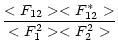
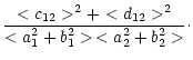
![\begin{displaymath}[C^2]_{xy}(f)
= \frac{[<c_{12}>^2]_{xy}+[<d_{12}>^2]_{xy}}
{[<a_1^2+b_1^2>\,<a_2^2+b_2^2>]_{xy}}\cdot
\end{displaymath}](/articles/aa/full/2001/45/aah2945/img56.gif)