A&A 379, L44-L47 (2001)
DOI: 10.1051/0004-6361:20011487
C. Alard1,2
1 - Institut d'Astrophysique de Paris, 98bis
boulevard Arago, 75014 Paris, France
2 -
Observatoire de Paris, 77 avenue Denfert Rochereau,
75014 Paris, France
Received 12 September 2001 / Accepted 22 October 2001
Abstract
A map of the projected density of the old stellar population
of the Galactic Bulge region is reconstructed using 2MASS data.
By making
a combination of the H and K photometric bands, it is possible to overcome the effect of reddening,
and thus penetrate the inner structure of the Galactic Bulge.
The main structure in the map corresponds to the well documented peanut shaped bar which is formed by the inner parts of the Galactic disk as a result of
dynamical instabilities.
As suggested by numerical simulations, the projected
Z profile of the bar, has
an almost exponential shape. After subtracting the
exponential profile associated with
the bar, a large residual appear near the Galactic Center. This
residual is elongated and asymmetrical, which suggest a bar structure.
Thus we arrive at the conclusion that in addition to the main bar
a smaller bar with a different orientation may exist in the
central region of the Milky Way.
This finding makes the Milky Way very similar to a large number of
barred spiral Galaxies which show as well a smaller bar
in their central regions.
Key words: Galaxy: bulge - Galaxy: structure
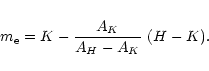
The 2MASS catalogues corresponding to the
range
![]() and
and
![]() were obtained from the 2MASS
public release. In this release the coverage of this coordinate
range is not complete (
were obtained from the 2MASS
public release. In this release the coverage of this coordinate
range is not complete (
![]() ), but is sufficient for
studies of Galactic structure.
The first step is to select the sources
with sufficient quality (read_flag>1). Using this criterion there are
about 30 millions stars in the region of interest. Within this area
there are a number of regions which are affected by the presence of
bright stars and their diffraction spikes.
It is easy to identify these areas since the star counts in the
neighborhood are much lower than average. By making
star counts in a box of 0.15 sq degree all over the frame,
we obtain an image where the regions occupied by bright stars appear
as dark patches. In case the counts in a box are less than 10, the relevant
pixel in the image is considered to belong to a dark patch. Even in the lower
density regions, the mean star counts are about 10 times larger, thus our
cut-off does not induce any artifact. To remove any contamination from
the dark spots to the nearby pixels, all the pixels belonging to a
), but is sufficient for
studies of Galactic structure.
The first step is to select the sources
with sufficient quality (read_flag>1). Using this criterion there are
about 30 millions stars in the region of interest. Within this area
there are a number of regions which are affected by the presence of
bright stars and their diffraction spikes.
It is easy to identify these areas since the star counts in the
neighborhood are much lower than average. By making
star counts in a box of 0.15 sq degree all over the frame,
we obtain an image where the regions occupied by bright stars appear
as dark patches. In case the counts in a box are less than 10, the relevant
pixel in the image is considered to belong to a dark patch. Even in the lower
density regions, the mean star counts are about 10 times larger, thus our
cut-off does not induce any artifact. To remove any contamination from
the dark spots to the nearby pixels, all the pixels belonging to a
![]() mesh were also flagged.
mesh were also flagged.
| (1) |
![\begin{figure}
\par\includegraphics[width=7.5cm,clip]{Fig1.eps} \end{figure}](/articles/aa/full/2001/45/aadi121/img14.gif) |
Figure 1: Here we present the polynomial smoothing of 2 sections of the projected density taken at constant longitude. Note that the profile deviates from an exponential near the Galactic Center. |
| Open with DEXTER | |
There is one major difficulty in
producing a map of the Bulge region: the coverage
is not complete and additionally there are holes due to
the bright stars. However provided that we assume that
the Galaxy is symmetrical about its plane, it is
possible to fill most of the gaps. In order to smooth
and fill the smaller data gaps which remain, we use
the fact that the density profile at constant longitude
is almost exponential (see Fig. 1). This property suggests that
the profile can be represented by a polynomial function.
Numerical experiments shows that it is not significant to
increase the degree of the polynomial beyond 5 to represent the data.
To increase the numerical stability of the fit we will use a strip
of 9 columns
centered around the column of interest. This procedure
is carried out for each column in the image. A filtered
image is constructed by replacing each column in the original
image by the polynomial solution. Some example of polynomial fitting
of the columns are given in Fig. 1. This procedure has a good ability
to fill or extrapolate small data gaps, and has an excellent numerical
stability. Once we have reconstructed this image of the star
counts in the Bulge region, we apply a final wavelet smoothing procedure in
order to balance the smoothing at all scales. This final smoothing
is interesting because the polynomial reconstruction is one dimensional,
and thus is biased in one direction, on a particular scale. The Wavelet
decomposition is obtained by applying iteratively the Spline
filter to the image and the smoothed images (Starck & Murtagh 1994).
To estimate
the statistical cuts to apply in the wavelet decomposition
we generate Monte-Carlo images with counts approaching our own image.
In the final reconstruction of the smoothed image we use 4![]() cuts.
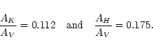
One final concern is the possible effect of
small uncertainties in the determination
of CK (typically a few %). This can be investigated by reconstructing
the density with small variations of CK. The comparison
with the initial map shows that the density variations induced by
such changes in the value of CK are about the amplitude
of the noise, and thus do not affect the final result.
cuts.
One final concern is the possible effect of
small uncertainties in the determination
of CK (typically a few %). This can be investigated by reconstructing
the density with small variations of CK. The comparison
with the initial map shows that the density variations induced by
such changes in the value of CK are about the amplitude
of the noise, and thus do not affect the final result.
![\begin{figure}
\par\includegraphics[width=8.8cm,clip]{Fig2.ps} \end{figure}](/articles/aa/full/2001/45/aadi121/img16.gif) |
Figure 2: Map of the Galactic Bar region reconstructed using a polynomial fitting method and wavelet smoothing. Note that the star counts are systematically higher at positive longitude for |b|>2. Contours values: (max,min)=(60000,400) stars/sq deg. |
| Open with DEXTER | |
We have already noticed that the Z profile of the projected density
is almost exponential. This exponential profile is also present in numerical
simulations of peanut shaped bars. Combes et al. (1990) showed that
a disk with a small bulge near its center forms a peanut
shaped bar with a nearly exponential projected Z profile (see in particular
Fig. 4 in Combes 1990). Thus if we
subtract the exponential contribution which corresponds to the bar-disk
system, the remaining density may reveal another component.
The contribution of the bar will be estimated by fitting an exponential
to each column of the image (which corresponds to the projected Z profile).
This procedure is more flexible than trying to subtract a bar model.
There are
still many uncertainties concerning the structure
of the Galactic bar, thus
the subtraction of a bar model may
give ambiguous results. By fitting an exponential
profile, we make no particular assumption about
the shape of the bar, other than
a general assumption on the Z profile at equilibrium which
is justified by numerical simulations.
To implement the fit of the exponential profile, we perform
a robust fitting of a straight line to the log of density
(by minimizing the sum of absolute deviations).
Once the exponential contribution
has been subtracted, a very significant residual appears
in the central region (![]() ). The contours of this
residual are smooth and elongated along the Galactic plane. This
component shows also a very significant asymmetry in longitude. The
amplitude of this asymmetry is close to 15%, which is about
7 sigmas according to Poisson statistics.
There are also some residuals along the Galactic plane in general.
But their amplitude is about 10 times smaller, they
do not have smooth structure, and their
scale is much smaller. These residuals are probably due to the presence of
young stars in the HII regions.
). The contours of this
residual are smooth and elongated along the Galactic plane. This
component shows also a very significant asymmetry in longitude. The
amplitude of this asymmetry is close to 15%, which is about
7 sigmas according to Poisson statistics.
There are also some residuals along the Galactic plane in general.
But their amplitude is about 10 times smaller, they
do not have smooth structure, and their
scale is much smaller. These residuals are probably due to the presence of
young stars in the HII regions.
![\begin{figure}
\par\includegraphics[width=8.8cm,clip]{Fig3.ps} \end{figure}](/articles/aa/full/2001/45/aadi121/img18.gif) |
Figure 3: Contours of the residual density after subtracting the main component. Note that the asymmetry is in the opposite direction of the large scale Galactic Bar. Contours values: (max,min)=(38000,400) stars/sq deg. |
| Open with DEXTER | |
There are some intrinsic difficulties in the interpretation of the
former results, we see a residual component after subtracting
a main component. But this result is based on the assumption that
the bar has a projected density profile in the Z direction which
is exponential. Even if this assumption is supported by numerical
simulations, it might just be that the projected density of the bar is
not exponential. But in this case, why do we observe an asymmetry
in an opposite direction to the bar?
Two possible sources of bias are: the residual extinction, and
the steepness of the density profile near the center (Blitz & Spergel 1991).
In principle the extinction should have no effect in the ![]() band,
but it is possible that for observational reasons the limiting magnitude
in 2MASS is somewhat brighter than expected, which would result in
an indirect extinction effect.
These biases can be investigated by using numerical simulations.
To build
a numerical model we need to integrate the convolution
product of the luminosity function
band,
but it is possible that for observational reasons the limiting magnitude
in 2MASS is somewhat brighter than expected, which would result in
an indirect extinction effect.
These biases can be investigated by using numerical simulations.
To build
a numerical model we need to integrate the convolution
product of the luminosity function ![]() with the density
distribution
with the density
distribution ![]() .
The integration domain in the
space of the magnitudes will be modulated by the extinction
AV. For the luminosity function
we will adopt the model of Wainscoat et al. (1992). The density
distribution will be built using a truncated exponential disk (Lopez-Corredoira et al. 2001) and a
triaxial bar model with a power law profile. This bar model has
an inclination of 20 deg with respect to the line of sight, and
axis ratio:
.
The integration domain in the
space of the magnitudes will be modulated by the extinction
AV. For the luminosity function
we will adopt the model of Wainscoat et al. (1992). The density
distribution will be built using a truncated exponential disk (Lopez-Corredoira et al. 2001) and a
triaxial bar model with a power law profile. This bar model has
an inclination of 20 deg with respect to the line of sight, and
axis ratio:
![]() and
and
![]() (Dwek et al. 1995). And finally the extinction map of the whole
area was built from our 2MASS data
by using a method presented by Schultheis et al. (2000).
Let's start with the case of residual extinction effects: the
counts were generated using the aforementioned procedure, Poisson noise was
simulated, and finally the whole process of polynomial reconstruction,
smoothing and exponential subtraction was applied. This procedure
was undertaken for different observational limiting magnitudes, starting
from our default value (no extinction cut-off). To summarize the
results, the longitude profile of the residual density has been
represented for the different limiting magnitude (Fig. 4).
(Dwek et al. 1995). And finally the extinction map of the whole
area was built from our 2MASS data
by using a method presented by Schultheis et al. (2000).
Let's start with the case of residual extinction effects: the
counts were generated using the aforementioned procedure, Poisson noise was
simulated, and finally the whole process of polynomial reconstruction,
smoothing and exponential subtraction was applied. This procedure
was undertaken for different observational limiting magnitudes, starting
from our default value (no extinction cut-off). To summarize the
results, the longitude profile of the residual density has been
represented for the different limiting magnitude (Fig. 4).
![\begin{figure}
\par\includegraphics[width=8.8cm,clip]{Fig4.ps} \end{figure}](/articles/aa/full/2001/45/aadi121/img24.gif) |
Figure 4: The marginal distribution in longitude of simulated profiles for different limiting magnitude (default: thin line, 1 mag brighter than default: dashed line, 1.5 mag brighter: dotted dashed line). The last profile is the observational profile (thick line). All profiles have been normalized so that the sum of the profile is unity. |
| Open with DEXTER | |