A. Jorissen1,![]() -
M. Mayor2 -
S. Udry2
-
M. Mayor2 -
S. Udry2
1 - Institut d'Astronomie et d'Astrophysique,
Université Libre de Bruxelles, CP 226, Boulevard du Triomphe,
1050
Bruxelles, Belgium
2 - Observatoire de Genève, 1290 Sauverny, Switzerland
Received 17 May 2001 / Accepted 24 September 2001
Abstract
The present study derives the distribution of secondary masses M2for the 67 exoplanets and very low-mass brown-dwarf companions of
solar-type stars, known as of April 4, 2001. This distribution is
related to the distribution of
![]() through an integral
equation of Abel's type. Although a formal solution exists for this
equation, it is known to be ill-conditioned, and is thus very sensitive to
the statistical noise present in the input
through an integral
equation of Abel's type. Although a formal solution exists for this
equation, it is known to be ill-conditioned, and is thus very sensitive to
the statistical noise present in the input
![]() distribution. To overcome this difficulty, we present two robust,
independent approaches: (i) the formal solution of the integral
equation is numerically computed after performing an optimal smoothing
of the input distribution and (ii) the Lucy-Richardson algorithm is used
to invert the integral equation. Both approaches give consistent
results. The resulting statistical distribution of exoplanet true
masses reveals that there is no reason to ascribe the transition
between giant planets and brown dwarfs to the threshold mass for
deuterium ignition (about 13.6
distribution. To overcome this difficulty, we present two robust,
independent approaches: (i) the formal solution of the integral
equation is numerically computed after performing an optimal smoothing
of the input distribution and (ii) the Lucy-Richardson algorithm is used
to invert the integral equation. Both approaches give consistent
results. The resulting statistical distribution of exoplanet true
masses reveals that there is no reason to ascribe the transition
between giant planets and brown dwarfs to the threshold mass for
deuterium ignition (about 13.6 ![]() ). The M2 distribution
shows instead that most of the objects have
). The M2 distribution
shows instead that most of the objects have
![]()
![]() ,
but there is a small tail with a few heavier candidates around
15
,
but there is a small tail with a few heavier candidates around
15 ![]() .
.
Key words: methods: numerical - stars: planetary systems
Han et al. (2001) suggested that most of the exoplanet candidates
discovered so far have masses well above the lower limit defined by
![]() (where i is the inclination of the orbital plane on the
sky) and should therefore be considered as brown dwarfs or even stars
rather than planets. The present paper shows that this claim is not
consistent with the distribution of masses extracted from the observed
(where i is the inclination of the orbital plane on the
sky) and should therefore be considered as brown dwarfs or even stars
rather than planets. The present paper shows that this claim is not
consistent with the distribution of masses extracted from the observed
![]() distribution (where M2 is the mass of the companion)
under the reasonable assumption that the orbits are oriented at random
in space. Although the distributions of M2 and
distribution (where M2 is the mass of the companion)
under the reasonable assumption that the orbits are oriented at random
in space. Although the distributions of M2 and
![]() are
related through an integral equation of Abel's kind
(Chandrasekhar & Münch 1950; Lucy 1974), its numerical solution is ill-conditioned. Two different methods are used here to overcome this
difficulty. In the first method (Sect. 2), the formal
solution of Abel's equation is implemented numerically on an input
are
related through an integral equation of Abel's kind
(Chandrasekhar & Münch 1950; Lucy 1974), its numerical solution is ill-conditioned. Two different methods are used here to overcome this
difficulty. In the first method (Sect. 2), the formal
solution of Abel's equation is implemented numerically on an input
![]() distribution that has been optimally smoothed with an
adaptive kernel procedure (Silverman 1986) to remove the
high-frequency fluctuations caused by small-number statistics. The
other method (Sect. 3) is based on the Lucy-Richardson
inversion algorithm (Richardson 1972; Lucy 1974).
distribution that has been optimally smoothed with an
adaptive kernel procedure (Silverman 1986) to remove the
high-frequency fluctuations caused by small-number statistics. The
other method (Sect. 3) is based on the Lucy-Richardson
inversion algorithm (Richardson 1972; Lucy 1974).
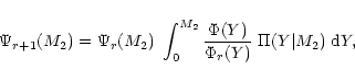
The basic reason why the M2 distribution obtained in Sect. 4 differs from that of Han et al. (2001) is because these authors concluded that most of the systems containing exoplanet candidates are seen nearly pole-on. This conclusion, based on the analysis of the Hipparcos Intermediate Astrometric Data (IAD), has however been shown to be incorrect (e.g. Halbwachs et al. 2000; Pourbaix 2001; Pourbaix & Arenou 2001), as summarized in Sect. 5.
While this paper was being reviewed, Zucker & Mazeh (2001) and Tabachnik & Tremaine (2001) proposed other interesting approaches to derive the exoplanet mass distribution. Zucker & Mazeh derive the binned true mass distribution by using a maximum likelihood approach to retrieve the average values of the mass distribution over the selected bins. Their results are in very good agreement with ours. Tabachnik & Tremaine suppose that the period and mass distributions follow power laws, and derive the corresponding power-law indices from a maximum likelihood method. On the contrary, the methods used in the present paper (and in Zucker & Mazeh's) are non-parametric in nature, since they do not require any a priori assumptions on the functional form of the mass distribution. This is especially important since the comparison of the shapes of the mass distributions for exoplanets and low-mass stellar companions may provide clues to identify the process by which they formed. By imposing a power-law function like that observed for low-mass stellar companions, Tabachnik & Tremaine (2001) implicitly assume that these processes must be similar.
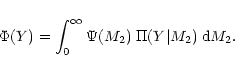
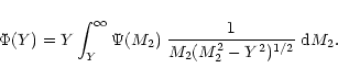
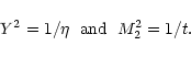
The
![]() values for low-mass companions of main sequence stars
may be extracted from the spectroscopic mass function and from the
primary mass as derived through e.g., isochrone fitting. Let
values for low-mass companions of main sequence stars
may be extracted from the spectroscopic mass function and from the
primary mass as derived through e.g., isochrone fitting. Let ![]() be the observed distribution of
be the observed distribution of
![]() ,
that is
easily derived from the observed spectroscopic mass functions provided
that
,
that is
easily derived from the observed spectroscopic mass functions provided
that
![]() as is expected to be the case for the systems
under consideration. Then, the distribution
as is expected to be the case for the systems
under consideration. Then, the distribution ![]() obeys
the relation
obeys
the relation
 |
(2) |
 |
(5) |
 |
(7) |
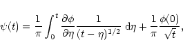
While Eq. (8) represents the formal solution of
the problem, it is difficult to implement numerically, since it
requires the differentiation of the observed frequency distribution
![]() .
Unless the observations are of high precision, it is well
known that this process can lead to misleading results. To overcome
this difficulty, the observed frequency distribution has been smoothed
in an optimal way (see Appendix) before being used in
Eq. (8). The solution
.
Unless the observations are of high precision, it is well
known that this process can lead to misleading results. To overcome
this difficulty, the observed frequency distribution has been smoothed
in an optimal way (see Appendix) before being used in
Eq. (8). The solution ![]() is then computed
numerically using standard differentiation and integration schemes.
is then computed
numerically using standard differentiation and integration schemes.
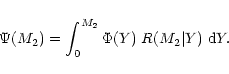
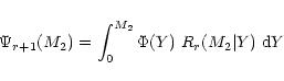
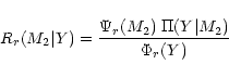
The Lucy-Richardson algorithm provides another robust way to invert
Eq. (4) (see also Cerf & Boffin 1994). The
method starts from the Bayes theorem on conditional probability in the
form
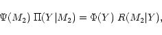 |
(9) |
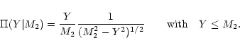
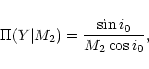
The reciprocal kernel represents the conditional probability that the
binary system has a companion mass M2 when the observed
![]() value amounts to Y. Thus, one has:
value amounts to Y. Thus, one has:
| R(M2|Y) | = | 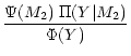 |
(11) |
| = | 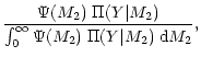 |
(12) |
 |
(15) |
When the number of data points is small
(typically N <100; Cerf & Boffin 1994), it is advantageous to express ![]() as
as
 |
(17) |
 |
(18) |
In the application of the method described in
Sect. 4, the initial mass distribution
![]() was taken as a uniform distribution, but it has been verified that this
choice has no influence on the final solution.
was taken as a uniform distribution, but it has been verified that this
choice has no influence on the final solution.
The cumulative frequency distribution of the
![]() values
smaller than 17
values
smaller than 17![]() ,
where
,
where ![]() is the mass of
Jupiter (=
is the mass of
Jupiter (=![]() /1047.35), available in the literature (as of April
4, 2001) is presented in Fig. 1. It appears to be
sufficiently well sampled to attempt the inversion procedure. The
corresponding frequency distributions smoothed with two different
smoothing lengths, locally self-adapting around
/1047.35), available in the literature (as of April
4, 2001) is presented in Fig. 1. It appears to be
sufficiently well sampled to attempt the inversion procedure. The
corresponding frequency distributions smoothed with two different
smoothing lengths, locally self-adapting around
![]()
![]() and 2
and 2
![]() (see Appendix) are presented
as well for comparison.
(see Appendix) are presented
as well for comparison.
![\begin{figure}
\par\includegraphics[width=8.8cm,clip]{MS1489fig1a.ps}\par\includegraphics[width=8.8cm,clip]{MS1489fig1b.ps}
\end{figure}](/articles/aa/full/2001/45/aa1489/img54.gif) |
Figure 1:
Bottom panel: the cumulative frequency distribution of the observed
|
| Open with DEXTER | |
The sample includes 60 main-sequence stars hosting 67 companions with
![]()
![]() .
Among those, 6 stars are orbited by
more than one companion, namely HD74156 and
HD82943
(
.
Among those, 6 stars are orbited by
more than one companion, namely HD74156 and
HD82943
(
![]() ,
7.40
,
7.40 ![]() ,
and
,
and
![]() ,
1.57
,
1.57 ![]() ,
respectively; Udry & Mayor 2001)
,
respectively; Udry & Mayor 2001)![]() ,
HD83433
(0.16,0.38
,
HD83433
(0.16,0.38 ![]() ;
Mayor et al. 2000),
HD168443
(7.22, 16.2
;
Mayor et al. 2000),
HD168443
(7.22, 16.2 ![]() ;
Udry et al. 2000b),
;
Udry et al. 2000b),
![]() And
(0.71, 2.20 and 4.45
And
(0.71, 2.20 and 4.45 ![]() ;
Butler et al. 1999) and
Gliese 876
(0.56, 1.88
;
Butler et al. 1999) and
Gliese 876
(0.56, 1.88 ![]() ;
Marcy et al. 2001).
The inversion process is only able to treat these systems under
the hypothesis that the orbits of the different planets in a given
system are not coplanar, since Eq. (4) to hold
requires random orbital inclinations. The case of coplanar and non-coplanar
orbits are discussed separately in the remainder of this section.
;
Marcy et al. 2001).
The inversion process is only able to treat these systems under
the hypothesis that the orbits of the different planets in a given
system are not coplanar, since Eq. (4) to hold
requires random orbital inclinations. The case of coplanar and non-coplanar
orbits are discussed separately in the remainder of this section.
Figure 2 compares the solutions ![]() obtained from
the Lucy-Richardson algorithm (after 2 and 20 iterations, denoted
obtained from
the Lucy-Richardson algorithm (after 2 and 20 iterations, denoted
![]() and
and ![]() ,
respectively) and from the formal solution
of Abel's integral equation with smoothing lengths
,
respectively) and from the formal solution
of Abel's integral equation with smoothing lengths
![]() and 2
and 2
![]() on
on ![]() (the corresponding solutions are denoted
(the corresponding solutions are denoted
![]() and
and
![]() ). The solutions from
the two methods basically agree with each other, although solutions
with different degrees of smoothness may be obtained with each method.
On the one hand,
). The solutions from
the two methods basically agree with each other, although solutions
with different degrees of smoothness may be obtained with each method.
On the one hand, ![]() and
and
![]() exhibit
high-frequency fluctuations that may be traced back to the statistical
fluctuations in the input data. This can be seen by noting that the
peaks present in
exhibit
high-frequency fluctuations that may be traced back to the statistical
fluctuations in the input data. This can be seen by noting that the
peaks present in
![]() correspond in fact to the
high-frequency fluctuations already present in
correspond in fact to the
high-frequency fluctuations already present in
![]() (Fig. 1). These fluctuations should thus not be given
much credit. The same explanation holds true for
(Fig. 1). These fluctuations should thus not be given
much credit. The same explanation holds true for ![]() ,
since it was argued in Sect. 3 that the solutions
,
since it was argued in Sect. 3 that the solutions ![]() resulting from a large number of iterations tend to match
resulting from a large number of iterations tend to match ![]() at
increasingly small scales (i.e., higher frequencies) where statistical
fluctuations become dominant. On the other hand,
at
increasingly small scales (i.e., higher frequencies) where statistical
fluctuations become dominant. On the other hand, ![]() and
and
![]() are much smoother, and are probably better
matches to the actual distribution. The local maximum
around
are much smoother, and are probably better
matches to the actual distribution. The local maximum
around
![]()
![]() is very likely, however,
an artifact of the strong
detection bias against low-mass companions.
is very likely, however,
an artifact of the strong
detection bias against low-mass companions.
![\begin{figure}
\par\includegraphics[width=8.8cm,clip]{MS1489fig2.ps}
\end{figure}](/articles/aa/full/2001/45/aa1489/img64.gif) |
Figure 2:
Comparison of |
| Open with DEXTER | |
The most striking feature of the ![]() distribution displayed in
Fig. 2 is its decreasing character, reaching zero for the
first time around M2 = 10
distribution displayed in
Fig. 2 is its decreasing character, reaching zero for the
first time around M2 = 10 ![]() ,
and in any case well before
13.6
,
and in any case well before
13.6 ![]() .
The latter value, corresponding to the minimum
stellar mass for igniting deuterium, does not in any way mark the
transition between giant planets and brown dwarfs, as sometimes
proposed. That transition, which is thus likely to occur at smaller
masses, must rely instead on the different mechanisms governing the
formation of planets and brown dwarfs. Another argument favouring a
giant-planet/brown-dwarf transition mass smaller than 13.6
.
The latter value, corresponding to the minimum
stellar mass for igniting deuterium, does not in any way mark the
transition between giant planets and brown dwarfs, as sometimes
proposed. That transition, which is thus likely to occur at smaller
masses, must rely instead on the different mechanisms governing the
formation of planets and brown dwarfs. Another argument favouring a
giant-planet/brown-dwarf transition mass smaller than 13.6 ![]() is provided e.g., by the observation of free-floating (and thus
most likely stellar) objects with masses probably smaller than
10
is provided e.g., by the observation of free-floating (and thus
most likely stellar) objects with masses probably smaller than
10 ![]() in the
in the ![]() Orionis star cluster
(Zapatero Osorio et al. 2000). The
Orionis star cluster
(Zapatero Osorio et al. 2000). The ![]() distribution nevertheless
clearly exhibits a tail of objects clustering around
distribution nevertheless
clearly exhibits a tail of objects clustering around
![]()
![]() ,
due to HD114762 (
,
due to HD114762 (
![]()
![]() ), HD162020 (14.3
), HD162020 (14.3 ![]() ),
HD202206 (15.0
),
HD202206 (15.0 ![]() )
and HD168443c
(16.2
)
and HD168443c
(16.2 ![]() ). It would be interesting to investigate whether
these systems differ from those with smaller masses in some
identifiable way (periods, eccentricities, metallicities, ...), so as
to assess whether or not they form a distinct class (Udry et al., in
preparation).
). It would be interesting to investigate whether
these systems differ from those with smaller masses in some
identifiable way (periods, eccentricities, metallicities, ...), so as
to assess whether or not they form a distinct class (Udry et al., in
preparation).
The jackknife method (e.g., Lupton 1993) has been used to
estimate the uncertainty on the
![]() solution. In a
first step, 67 input
solution. In a
first step, 67 input
![]() distributions are
computed, corresponding to all 67 possible sets with one data point
removed from the original set. Equation (8) is then
applied to these 67 different input distributions. The resulting
distributions are displayed in Fig. 3, which shows
that the threshold observed at 10
distributions are
computed, corresponding to all 67 possible sets with one data point
removed from the original set. Equation (8) is then
applied to these 67 different input distributions. The resulting
distributions are displayed in Fig. 3, which shows
that the threshold observed at 10 ![]() is a robust result not
affected by the uncertainty on the solution.
is a robust result not
affected by the uncertainty on the solution.
![\begin{figure}
\par\includegraphics[width=8.8cm,clip]{MS1489fig3.ps}
\end{figure}](/articles/aa/full/2001/45/aa1489/img68.gif) |
Figure 3:
Comparison of the input
|
| Open with DEXTER | |
All the results discussed so far are obtained under the assumption
that orbits of planets belonging to a planetary system are not
coplanar. To evaluate the impact of this hypothesis, the following
procedure has been applied. In a first step, the Lucy-Richardson
algorithm is applied on the data set excluding the 13 planets
belonging to planetary systems. That mass distribution obtained after
2 iterations is then completed by mass estimates for the remaining 13
planets. For each of the 6 different systems, an inclination i is
drawn from a ![]() distribution. This is done through the
expression
distribution. This is done through the
expression
![]() ,
where x is a random number with
uniform deviation. The same value of i is then applied to all planets
in a given system to extract M2 from the observed
,
where x is a random number with
uniform deviation. The same value of i is then applied to all planets
in a given system to extract M2 from the observed
![]() value. The distributions of exoplanet masses obtained with and
without the hypothesis of coplanarity are compared in
Fig. 4, and it is seen that planetary systems are not
yet numerous enough for the coplanarity hypothesis to alter
significantly the resulting
value. The distributions of exoplanet masses obtained with and
without the hypothesis of coplanarity are compared in
Fig. 4, and it is seen that planetary systems are not
yet numerous enough for the coplanarity hypothesis to alter
significantly the resulting ![]() distribution.
distribution.
![\begin{figure}
\par\includegraphics[width=8.8cm,clip]{MS1489fig4.ps}
\end{figure}](/articles/aa/full/2001/45/aa1489/img70.gif) |
Figure 4:
Evaluation of the impact of the coplanarity hypothesis on the
resulting |
| Open with DEXTER | |
In any case, the main result of the present paper is that the statistical properties of the observed
![]() distribution
coupled with the hypothesis of randomly oriented orbital planes
confine the vast majority of planetary companion masses below about 10
distribution
coupled with the hypothesis of randomly oriented orbital planes
confine the vast majority of planetary companion masses below about 10 ![]() .
Zucker & Mazeh (2001) reach the same conclusion.
.
Zucker & Mazeh (2001) reach the same conclusion.
It should be remarked that the above conclusion cannot be due to detection biases, since the high-mass tail of the M2 distribution is not affected by the difficulty of finding low-amplitude, long-period orbits.
Although the assumption of random orbital inclinations seems
reasonable, it is at variance with the conclusion of
Han et al. (2001) that most of the systems containing exoplanet
candidates are seen nearly pole-on. These authors reached this
conclusion by trying to extract the astrometric orbit, hence the
orbital inclination, from the Hipparcos IAD. Halbwachs et al. (2000)
had already cautioned that this approach is doomed to fail for systems
with apparent separations on the sky that are below the Hipparcos
sensitivity (i.e.
![]() 1 mas). In those cases, the solution retrieved
from the fit of the IAD residuals is spurious, since the true angular
semi-major axis a is simply too small to be seen by Hipparcos. Since
Halbwachs et al. (2000) have shown that a actually follows a
Rayleigh probability distribution, the fit of the IAD residuals will
yield a solution larger than the true value, in fact of the order of
the residuals. But since
1 mas). In those cases, the solution retrieved
from the fit of the IAD residuals is spurious, since the true angular
semi-major axis a is simply too small to be seen by Hipparcos. Since
Halbwachs et al. (2000) have shown that a actually follows a
Rayleigh probability distribution, the fit of the IAD residuals will
yield a solution larger than the true value, in fact of the order of
the residuals. But since ![]() is constrained by the
spectroscopic orbital elements, the too-large astrometric a value
will force i to be close to 0 to match the spectroscopic value of
the product
is constrained by the
spectroscopic orbital elements, the too-large astrometric a value
will force i to be close to 0 to match the spectroscopic value of
the product ![]() ,
as convincingly shown by
Pourbaix (2001). Hence, this approach gives the impression
that all orbits are seen nearly face-on. As an illustrative example,
Pourbaix & Arenou (2001) have shown that such an approach leads to a
stellar mass for the companion of HD209458 that, on another hand,
has been proven to be a 0.69
,
as convincingly shown by
Pourbaix (2001). Hence, this approach gives the impression
that all orbits are seen nearly face-on. As an illustrative example,
Pourbaix & Arenou (2001) have shown that such an approach leads to a
stellar mass for the companion of HD209458 that, on another hand,
has been proven to be a 0.69![]() planet by the photometric
observation of the planet transit in front of the star
(Charbonneau et al. 2000).
planet by the photometric
observation of the planet transit in front of the star
(Charbonneau et al. 2000).
The Han et al. (2001) result is moreover statistically very
unlikely if the orbital planes are oriented at random in space
(Pourbaix & Arenou 2001). Han et al. (2001) have tried to justify this
unlikely statistical occurrence by invoking biases against
high-amplitude orbits in the selection
process of the radial-velocity-monitoring samples. To the contrary,
the planet-search surveys were specifically devised to avoid such biases, as
they aim at finding not only giant planets but also brown dwarfs
so as to constrain the substellar secondary mass function
of solar-type stars.
Furthermore, the Han et al. (2001) argument
is totally invalid in the case of volume-limited, statistically well-defined
samples like that of the CORALIE planet-search programme in the southern
hemisphere (Udry et al. 2000a). This sample has been specifically
designed to detect companions
of solar-type stars all the way from
q=M2/M1 = 1 down to
![]() .
.
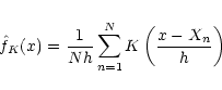
To decrease the noise and allow a tractable use of the information present in small data samples, heavy smoothing techniques are often required. A common practice consists converting a set of discrete positions into binned "counts''. Binning is a crude sort of smoothing and many studies in statistical analysis have shown that, unless the smoothing is done in an optimum way, some, or even most, of the information content of the data could be lost. This is especially true when a large amount of smoothing is necessary, which then changes the "shape'' of the resulting function. In statistical terms, the smoothing process not only decreases the noise (i.e., the function's variance), but at the same time introduces a bias in the estimate of the function.
The variance-bias trade off is unavoidable but, for a given level of variance, the bias increase can be minimized. The correct manner of achieving that task is provided by the so-called non-parametric density estimate methods for the determination of the "frequency'' function of a given parameter or by the non-parametric regression methods for the determination of a smooth function ginferred from direct measurements of g itself. Moreover, adaptive non-parametric methods are designed to filter the data in some local, objective way minimizing the bias, in order to get the smooth desired function without constraining its form in any way. The theory and algorithms related to those methods, originally built to handle ill-conditioned problems (either under-determined or extremely sensitive to errors or incompleteness in the data), are widely discussed in the specialized literature and summarized in easy-to-read textbooks (e.g., Silverman 1986; Härdle 1990; Scott 1992).
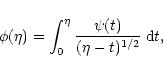
The simplest of the available algorithms is provided by the kernel
estimator leading to the following form of the normalized
"frequency'' function
 |
(20) |
In the adaptive kernel version, a local bandwidth
hn=h(Xn,f) is defined and used in Eq. (19). In order to
follow the "true'' underlying function in the best possible way, the
amount of smoothing should be small when f is large whereas more
smoothing is needed where f takes lower values. A convenient method
to do so consists in deriving first a pilot estimate ![]() of f, e.g. by
using an histogram or a kernel with fixed bandwidth
of f, e.g. by
using an histogram or a kernel with fixed bandwidth
![]() ,
and
then by defining the local bandwidths
,
and
then by defining the local bandwidths
![\begin{displaymath}h_n=h(X_n)=h_{\rm opt}[\tilde f(X_n)/s]^{-\alpha},
\end{displaymath}](/articles/aa/full/2001/45/aa1489/img78.gif) |
(21) |
 |
(22) |
The optimum kernel K may be taken as the one minimizing the integrated
mean square error beween f and ![]() (MISE), where
(MISE), where
![\begin{displaymath}{\rm MISE}(\hat{f}) = E\int\left[ \hat{f}(x) - f(x) \right]^2 {\rm d}x
\end{displaymath}](/articles/aa/full/2001/45/aa1489/img82.gif) |
(23) |
 |
(24) |
The pilot smoothing length (
![]() )
is the only subjective
parameter required by the method. It relates to the quality of the
sampling of the variable under consideration. There are several ways for
automatically estimating an optimum value of
)
is the only subjective
parameter required by the method. It relates to the quality of the
sampling of the variable under consideration. There are several ways for
automatically estimating an optimum value of
![]() (see e.g. Silverman 1986 for an extensive review). A simple approach based
on the data variance gives in our case
(see e.g. Silverman 1986 for an extensive review). A simple approach based
on the data variance gives in our case
![]()
![]() .
As the derivative of the frequency function rather than the
function itself is actually used in
Eq. (6), a larger pilot smoothing length (
.
As the derivative of the frequency function rather than the
function itself is actually used in
Eq. (6), a larger pilot smoothing length (
![]() )
was
also considered in order to remove spurious small-statistics
fluctuations of the density estimate.
)
was
also considered in order to remove spurious small-statistics
fluctuations of the density estimate.