A&A 379, 1138-1152 (2001)
DOI: 10.1051/0004-6361:20011405
Formation of a proto-quasar from accretion flows in a halo
A. Mangalam
Indian Institute of Astrophysics, Koramangala, Bangalore 560034, India
Received 23 April 2001 / Accepted 4 October 2001
Abstract
We present a detailed model for the formation of massive objects at
the centers of galaxies. The effects of supernovae heating and the
conditions of gas loss are revisited. The escape time of the gas is
compared with the cooling time, which provides an additional condition
not previously considered. Its consequences for the allowed mass
range of the halo is calculated and parameterized in terms of the
spin parameter,
 ,
the redshift of collapse,
,
the redshift of collapse,  ,
the
fraction of baryons in stars,
,
the
fraction of baryons in stars,  ,
and the efficiency of
supernovae,
,
and the efficiency of
supernovae,  .
It is shown that sufficient gas is retained to
form massive dark objects and quasars even for moderately massive
halos but a decline is expected at low redshifts. Subsequently, a
gaseous disk forms with a radial extent of a kpc, spun up by tidal
torques and magnetized by supernovae fields with fields strengths of
10-100
.
It is shown that sufficient gas is retained to
form massive dark objects and quasars even for moderately massive
halos but a decline is expected at low redshifts. Subsequently, a
gaseous disk forms with a radial extent of a kpc, spun up by tidal
torques and magnetized by supernovae fields with fields strengths of
10-100  .
In a model of a self-similar accretion flow in an
initially dominant halo, it is shown that for typical halo
parameters, about
.
In a model of a self-similar accretion flow in an
initially dominant halo, it is shown that for typical halo
parameters, about
 accretes via small magnetic
stresses (or alternatively by self-gravity induced instability or by
alpha viscosity) in 108 years into a compact region. A model of a
self-gravitating evolution of a compact magnetized disk (
accretes via small magnetic
stresses (or alternatively by self-gravity induced instability or by
alpha viscosity) in 108 years into a compact region. A model of a
self-gravitating evolution of a compact magnetized disk (
 pc), which is relevant when a significant fraction of the disk
mass falls in, is presented, and it has a rapid collapse time scale
of a million years. The two disk solutions, one for accretion in an
imposed halo potential and the other for a self-gravitating disk,
obtained here, have general utility and can be adapted to other
contexts like protostellar disks as well. Implications of this work
for dwarf galaxy formation, and a
residual large scale seed field, are also breifly discussed.
pc), which is relevant when a significant fraction of the disk
mass falls in, is presented, and it has a rapid collapse time scale
of a million years. The two disk solutions, one for accretion in an
imposed halo potential and the other for a self-gravitating disk,
obtained here, have general utility and can be adapted to other
contexts like protostellar disks as well. Implications of this work
for dwarf galaxy formation, and a
residual large scale seed field, are also breifly discussed.
Key words: accretion, accretion disks - magnetic fields - galaxies: formation - cosmology: theory
There seems to be increasing evidence that supermassive black holes
are at the centers of galaxies. Dynamical searches indicate the
existence of massive dark objects (MDOs) in eight systems and their
masses range from 106-
 (Kormendy & Richstone
1995). Although this study does not confirm that the central objects
are supermassive black holes, it has been inferred that the central
mass is contained within 105 Schwarzchild radii.
On an average,
the black hole mass is a fraction, 10-2-10-3, of the total
mass of the galaxy and of order 10-3.5 of the bulge mass (Wandel 1999). Recent observations show a strong correlation between the
black hole mass,
(Kormendy & Richstone
1995). Although this study does not confirm that the central objects
are supermassive black holes, it has been inferred that the central
mass is contained within 105 Schwarzchild radii.
On an average,
the black hole mass is a fraction, 10-2-10-3, of the total
mass of the galaxy and of order 10-3.5 of the bulge mass (Wandel 1999). Recent observations show a strong correlation between the
black hole mass,
 ,
from stellar dynamical estimates, and the velocity dispersion of the host bulges (
,
from stellar dynamical estimates, and the velocity dispersion of the host bulges (
 ;
where
;
where  is reported to be in the range 3.5-5; e.g. Ferrarese & Merritt 2000). This has been supported by reverberation mapping studies of the broad line region (Gebhardt et al. 2000). The black hole masses in active galaxies as inferred from their luminosities, assuming reasonable efficiencies, are also in the same range,
 .
Arguments based on time variability, relativistic jets and other circumstantial evidence indicate that they are relativistically compact (Blandford & Rees
1992). Specific examples include a
.
Arguments based on time variability, relativistic jets and other circumstantial evidence indicate that they are relativistically compact (Blandford & Rees
1992). Specific examples include a  20 pc disk spining at 500 km s-1 which implies a
 black hole in M 87 (Ford et al. 1994) and evidence of
 mass in a region of 0.1 pc in the case of NGC 4258 (Miyoshi et al.
1995). One remarkable fact is that there is a decline in the quasar
population between z=2 and the present epoch. The presence of
quasars at high redshifts tells us that galaxy formation had proceeded
far enough for supermassive black holes to form in the standard
picture (Rees 1984). A detailed model of formation of these objects,
such as the one attempted here, should address the issues of
supernovae feedback from star formation and the mechanism of efficient
angular momentum transport in order to explain the massive active
nuclei as early as z=5. In the case of MDOs, there is a need to
explain the compact sizes of 10-100 pc that are implied from dynamical studies.
mass in a region of 0.1 pc in the case of NGC 4258 (Miyoshi et al.
1995). One remarkable fact is that there is a decline in the quasar
population between z=2 and the present epoch. The presence of
quasars at high redshifts tells us that galaxy formation had proceeded
far enough for supermassive black holes to form in the standard
picture (Rees 1984). A detailed model of formation of these objects,
such as the one attempted here, should address the issues of
supernovae feedback from star formation and the mechanism of efficient
angular momentum transport in order to explain the massive active
nuclei as early as z=5. In the case of MDOs, there is a need to
explain the compact sizes of 10-100 pc that are implied from dynamical studies.
Broadly, the two main routes to the formation of the massive central
objects that have been proposed are through instabilities in a
relativistic stellar cluster or gas dynamical schemes which may
involve a direct collapse of a primordial gas cloud or accretion of a
collapsed gaseous disk. The main drawback of the stellar cluster models is that one must assume the existence of a dense and massive cluster at the outset; the angular momentum transport problem to arrive at this initial scenario is difficult to overcome. One gas dynamical scheme proposed by Shlosman et al. (1990) involves accretion
of gas through stellar bars which have been induced either by self-gravity or
galaxy interactions driving the gas from 10 kpc to about a kpc size "disk of clouds" which further accretes by viscous dissipation due to cloud-cloud collisions. N-body
simulations (Sellwood & Moore 1998) have shown that the bar weakens
substantially after a few percent of the disk mass accumulates in the
center. This mechanism may not last long enough to drive sufficient
matter into a compact region as the bar instability is suppressed by
the bulge at the inner Linblad resonance. Disk accretion due
to self-gravity and magnetic fields may then be better candidates to
transport the mass to about a 100 pc size compact region.
Loeb & Rasio (1994) considered the possibility that massive black holes form
directly during the intial collapse of the protogalaxies at high redshifts and
performed smoothed particle
hydrodynamical simulations of gas clouds. They find that inital collapse of
a protogalactic cloud leads to the formation of a rotatinally supported
thin disk. They argue that if the viscous transport time in the disk is small
compared to the cooling time, then the disk could collapse to a supermassive star,
else it could form a supermassive disk; they do not provide
gas dynamical collapse model after the formation of a disk or star. They found that the gas
fragments into small dense clumps (presumably are converted into
stars). The important
consequences of supernovae feedback is not considered. Eisentein & Loeb (1995) suggest that quasars may be associated with rare systems that
acquire low values of angular momentum from tidal torques during the
cosmological collapse. Typically these are
 objects and form at
redshifts
objects and form at
redshifts
 .
Since the viscous evolution times in the collapsed
disks of these objects are comparable to star formation times, it is important
to consider the effects of supernovae feedback in detail that could disrupt
these objects.
.
Since the viscous evolution times in the collapsed
disks of these objects are comparable to star formation times, it is important
to consider the effects of supernovae feedback in detail that could disrupt
these objects.
Natarajan (1999) considers the effect of feedback and argues that the fraction
of the gas retained is proportional to ratio of the supernovae heat input to
the binding energy of the gas in the halo. This assumption has interesting
consequences for the Tully-Fisher relationship. The criteria for mass loss
was considered by Mac-Low & Ferrara (1999), Ferrara & Tolstoy (2000)
in the context of a blow-out or a blow-away (when the mass is completely expelled) from disk galaxy with an isothermal atmosphere. The condition for the gas to be retained is that the blow-out velocity be less than the escape velocity. However, the cooling of the hot gas is not considered. In this paper,
we consider the possibility that gas cools before it escapes the halo.
Silk & Rees (1998) propose that 10
 clouds at high redshifts undergo direct collapse in a hierarchical (bottom-up) CDM cosmology without undergoing fragmentation and star formation arguing that the conditions in primordial clouds differ from conventional molecular clouds. The angular momentum in this picture is shed by non-axisymmetric gravitational instabilities. The more massive black holes
(
)
ejects mass from the host galaxies by assumed spherical quasar winds. In the limiting case, it provides a relationship between the mass of the central hole and the host galaxy mass. The time between halo
virialization and the birth of quasars is short compared to the
cosmological timescale. Haehnelt & Rees (1993) proposed a scenario
in which a disk forms (after turnaround and collapse) and loses
angular momentum due to
viscosity in an estimated timescale
of 108 yrs.
clouds at high redshifts undergo direct collapse in a hierarchical (bottom-up) CDM cosmology without undergoing fragmentation and star formation arguing that the conditions in primordial clouds differ from conventional molecular clouds. The angular momentum in this picture is shed by non-axisymmetric gravitational instabilities. The more massive black holes
(
)
ejects mass from the host galaxies by assumed spherical quasar winds. In the limiting case, it provides a relationship between the mass of the central hole and the host galaxy mass. The time between halo
virialization and the birth of quasars is short compared to the
cosmological timescale. Haehnelt & Rees (1993) proposed a scenario
in which a disk forms (after turnaround and collapse) and loses
angular momentum due to
viscosity in an estimated timescale
of 108 yrs.
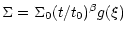
![\begin{figure}
\par\includegraphics[width=8.8cm,clip]{MS1409f1.eps}\end{figure}](/articles/aa/full/2001/45/aa1409/Timg45.gif) |
Figure 1:
The evolution of a
 cloud leading to a formation of a
protoquasar. In first step, this cloud cools faster than the dynamical time,
cloud leading to a formation of a
protoquasar. In first step, this cloud cools faster than the dynamical time,
 .
After star formation, one of the conditions is satisfied- that the supernovae heat energy is less than the binding energy, .
After star formation, one of the conditions is satisfied- that the supernovae heat energy is less than the binding energy,
 or that the cooling time of the hot gas is less than the time to escape the halo,
 . . |
| Open with DEXTER |
Here, we discuss a detailed physical model for the formation of protoquasars
(or MDOs) from a magnetized accretion of a collapsed disk, the
properties of which are obtained taking into account supernovae
feedback in a virialized halo. There is observational evidence that
considerable fragmentation precedes quasar activity and the broad
emission lines in quasar spectra indicate high metallicity (Hamann &
Ferland 1992). We assume, therefore, significant star formation and
supernovae activity occurs after the cloud, which is spun up by tidal
torques, contracts to a radius where self-gravity is significant. The
paper is composed of the following parts (see Fig. 1).
- 1.
-
The formation of a gaseous disk
with a radial extent of about a kpc, in a host galaxy as limited by supernovae feed back. We
investigate in Sect. 2, the range in halo mass for a given
redshift that still retains the hot gas. The effect of the
evolution of gas on the collisionless dark matter system is neglected;
- 2.
-
In previous work, gravitational instabilities (examined in Sect. 4.3)
in the disk was considered as the main source of viscosity. In Sect. 4.1,
justification is made for a magnetic viscosity from supernovae fields
and the estimated accretion rate turns out to be significant; also the large scale field strength derived from the
effective seed of small scale fields is used to explain observations (Sect. 3);
- 3.
-
The collapse of the disk is calculated with a generalized viscosity
prescription (which includes the individual cases of magnetic,
and self-gravity induced instabilities, Sect. 4) under a halo
dominated gravitational potential (Sect. 5) into a compact central region at rapid rate of about a
 .
A self-gravitating magnetized disk solution for this central
object that collapses in 106 yrs, is presented in Sect. 6. There is summary and discussion in Sect. 7 and conclusions in Sect. 8.
.
A self-gravitating magnetized disk solution for this central
object that collapses in 106 yrs, is presented in Sect. 6. There is summary and discussion in Sect. 7 and conclusions in Sect. 8.
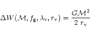
2 The virialized spherical halo and formation of the gaseous disk
We assume a standard spherical model for the formation of a virialized
spherical halo to begin with, in which the gas cools to form the
disk. Subsequently, we include in the calculations the supernovae
heating and consider the conditions under which sufficient gas is
retained to form the disk.
A particularly simple and useful version of the spherical model below
assumes that the matter distribution is symmetric about a point and is
a pressureless fluid. The shell enclosing mass of the overdense
region,  ,
initially expands with the background universe, slows
down, reaches a maximum radius before it turns around, and
collapses. The collapse proceeds until a time when it reaches virial
equilibrium. For an average density contrast,
,
initially expands with the background universe, slows
down, reaches a maximum radius before it turns around, and
collapses. The collapse proceeds until a time when it reaches virial
equilibrium. For an average density contrast,  ,
and using the
fact that the background density,
,
and using the
fact that the background density,
 for a flat
cosmological model, one can make the following estimates of the
typical parameters of the collapsed object (Padmanabhan & Subramanian 1992; Padmanabhan 1993; Peebles 1980)
for a flat
cosmological model, one can make the following estimates of the
typical parameters of the collapsed object (Padmanabhan & Subramanian 1992; Padmanabhan 1993; Peebles 1980)
where  and
and  are the current values of the comoving
density and time, the subscripts t and c indicate turn around and
collapse values, and
are the current values of the comoving
density and time, the subscripts t and c indicate turn around and
collapse values, and  is the radius of virialization. For a given
model of the cosmological evolution of the initial density
perturbation, one obtains values for
is the radius of virialization. For a given
model of the cosmological evolution of the initial density
perturbation, one obtains values for  or alternatively one
can specify the collapse redshift. As an example,
or alternatively one
can specify the collapse redshift. As an example,
 corresponds to
 and a
and a
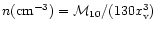
 7.8. We take
 and the mass in baryons, M9, in units of
 ,
is related to the total mass by
,
is related to the total mass by
 |
(2) |
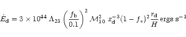
The baryonic mass, M9, will fuel a black hole, after it has formed,
at a rate limited by the Eddington luminosity. If the accretion
proceeds at a tenth of this rate, then the luminosity in units of
 is
is
 |
(3) |
where
 is the mass of the black hole in units of
.
is the mass of the black hole in units of
.
Calculation of the collapse factor

The gas in the massive dark halo of size
radiative cools to form
a disk of radial extent  .
Before we consider the details of
cooling in Sect. 2.2, we first need to estimate the collapse
factor,
.
Before we consider the details of
cooling in Sect. 2.2, we first need to estimate the collapse
factor,
 ,
which is based upon the conservation of angular
momentum. The disk forms when the gas becomes rotationally
supported. The protoquasar acquires its spin from tidal torques of its
neighbors and N-body simulations (Barnes & Efsthaiou 1987) and
analytical studies (Heavens & Peacock 1988) indicate that the spin
parameter of the virialized system,
,
to be in the range
0.01-0.1. If the angular momentum is conserved and there is no
exchange between the gas and dark components, the ratio of angular
momentum in the gas to the halo would remain as
,
which is based upon the conservation of angular
momentum. The disk forms when the gas becomes rotationally
supported. The protoquasar acquires its spin from tidal torques of its
neighbors and N-body simulations (Barnes & Efsthaiou 1987) and
analytical studies (Heavens & Peacock 1988) indicate that the spin
parameter of the virialized system,
,
to be in the range
0.01-0.1. If the angular momentum is conserved and there is no
exchange between the gas and dark components, the ratio of angular
momentum in the gas to the halo would remain as
 ,
so that
,
so that
 |
(4) |
where
 is the spin parameter,
L is the angular mometum, and
is the spin parameter,
L is the angular mometum, and
 and
and
 are the binding energies in the halo and
the disk respectively. If the halo has a constant density then
k1=0.3 and if it were a truncated isothermal sphere then k1=0.5.
Using the form for the circular velocity,
are the binding energies in the halo and
the disk respectively. If the halo has a constant density then
k1=0.3 and if it were a truncated isothermal sphere then k1=0.5.
Using the form for the circular velocity,
 ,
of
a disk spinning in an isothermal halo and taking the angular momentum
of the disk to be equal to
,
of
a disk spinning in an isothermal halo and taking the angular momentum
of the disk to be equal to
 ,
where s is a geometrical
factor (typically of order unity; s=2 for an exponential disk) that
depends on the mass distribution in the disk, the radial extent of the
disk is given by
,
where s is a geometrical
factor (typically of order unity; s=2 for an exponential disk) that
depends on the mass distribution in the disk, the radial extent of the
disk is given by
 |
(5) |
Typically, the disk size is a tenth of the virial radius, and the
collapse factor ranges from 10 to 20. For convenience we make the
following definitions
 |
(6) |
 |
(7) |
where
is the radius of the disk.
2.2 Cooling
In order that gaseous disks (with collapse factor estimated above)
form in the halo where star formation and supernovae take place, it is
important to examine whether the gas can be retained in the hosts in
the first place. In this section, we examine the constraints on black
hole hosts (those that can retain the gas) from star formation and gas
loss due to supernovae. Consider a virialized halo which contracts
due to cooling to a radius where it fragments due to self-gravity and
star formation takes place. Below we list the conditions that specify
when a halo condenses to form stars, whether the gas becomes unbound
due to supernovae heating and finally whether the gas cools before it
can escape and hence remains trapped in the halo. The first two of the
conditions were considered earlier and in this paper we introduce a
third necessary condition previously not considered.
C0. Following earlier work (e.g. White & Rees 1979; Rees & Ostriker 1977; Silk 1977), we state the condition that a luminous core can form in a halo
 |
(8) |
where  is the cooling time and
  is the dynamical time.
The
heating process by was examined in some detail by Dekel & Silk (1986,
DS) in the context of dwarf galaxies; they found that a condition of
gas loss amounted to the virial velocity being below a certain
critical velocity. At a time,
is the dynamical time.
The
heating process by was examined in some detail by Dekel & Silk (1986,
DS) in the context of dwarf galaxies; they found that a condition of
gas loss amounted to the virial velocity being below a certain
critical velocity. At a time,  ,
when the hot gas in supernovae
shells significantly fills up the volume under consideration, the
following constraints should be satisfied.
,
when the hot gas in supernovae
shells significantly fills up the volume under consideration, the
following constraints should be satisfied.
C1. As given by DS, the effective heat input
by supernovae is
 |
(9) |
where  is the gas fraction in the total mass and
  is the
circular (or virial) velocity in the halo. This implies that the
supernovae heat input should be greater the binding energy for the gas
to escape.
is the
circular (or virial) velocity in the halo. This implies that the
supernovae heat input should be greater the binding energy for the gas
to escape.
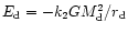
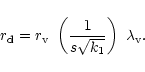
C2. We find that an additional condition
for gas loss is necessary, namely, that the time for the hot gas to
cool should be longer than the escape time,  of the system
 |
(10) |
where
is approximated by the time scale
 |
(11) |
where
 represents the mean kinetic energy per unit mass
and
represents the mean kinetic energy per unit mass
and  is the mean gravitational potential per unit mass. In
other words, even if supernovae heat input causes the gas to become
unbound, it can still be trapped in the halo if it cools faster than
the time required to escape, which is of the order of the dynamical
time.
is the mean gravitational potential per unit mass. In
other words, even if supernovae heat input causes the gas to become
unbound, it can still be trapped in the halo if it cools faster than
the time required to escape, which is of the order of the dynamical
time.
In order to quantify these physical constraints, we have to calculate
 ,
the effective heat input by supernovae. The standard
evolution of a supernova remnant goes through two phases- adiabatic
and radiative. In the adiabatic phase (Sedov-Taylor), the radiation
loss is negligible and the time at which the shock front radiates
about three-quarters of its initial energy is given by DS as
,
the effective heat input by supernovae. The standard
evolution of a supernova remnant goes through two phases- adiabatic
and radiative. In the adiabatic phase (Sedov-Taylor), the radiation
loss is negligible and the time at which the shock front radiates
about three-quarters of its initial energy is given by DS as
 |
(12) |
where n is the ambient hydrogen number density in cm-3. As a
result, the input into the gas equals the initial energy minus the
radiative losses in the adiabatic phase and subsequently for later
times, the gas is cooled by expansion. The cumulative energy input
from the supernovae at a given time, t, will be dominated by those
that have exploded within a time
 before t. The star
formation rate is taken to be a constant and is approximately,
before t. The star
formation rate is taken to be a constant and is approximately,
 ,
where
is the baryonic mass fraction in stars and
further, it is assumed that the star formation abruptly ends at
,
where
is the baryonic mass fraction in stars and
further, it is assumed that the star formation abruptly ends at
 .
The IMF of the solar neighborhood gives rise to one supernova
per 200
.
The IMF of the solar neighborhood gives rise to one supernova
per 200  of newly formed stars. If
  is the number
of supernova explosions per
is the number
of supernova explosions per
 of newly formed
stars
of newly formed
stars![[*]](/icons/foot_motif.gif) with each explosion releasing
with each explosion releasing
 ergs
of initial energy, then the energy input into the gas is then given by
ergs
of initial energy, then the energy input into the gas is then given by
 |
(13) |
and the dynamical time for the system is a quarter of the oscillation
period given by
 |
(14) |
which is assumed to set the timescale for star formation. Also,
f(t), is a function of time that is of order unity and its form is
given by Eq. (45) in DS
![\begin{displaymath}f(t)= \left \{ \begin{array}{cc} (t/t_{\rm rad}) [1-0.14
(t/...
...t_{\rm rad})^{0.38} -1] & t > t_{\rm rad}. \end{array} \right.
\end{displaymath}](/articles/aa/full/2001/45/aa1409/img109.gif) |
(15) |
The ratio
 implies that
f(t) is of order unity and
0 < f(t) < 3.6 (for
implies that
f(t) is of order unity and
0 < f(t) < 3.6 (for
 ). The
heat input from the supernovae that have exploded within a time,
,
of a given instant are the most effective in contributing
to the heating. Now the shells of the supernovae will start filling
up the volume. The time at which hot gas has a filling factor of order
unity (
). The
heat input from the supernovae that have exploded within a time,
,
of a given instant are the most effective in contributing
to the heating. Now the shells of the supernovae will start filling
up the volume. The time at which hot gas has a filling factor of order
unity (
 ), is estimated in the following manner.
2.3 Filling factor of SNR
We use the well-known simple expressions (e.g. Spitzer 1978) for the
advance of the supernova through the Sedov-Taylor and snow-plow phases
in a medium whose number density of hydrogen is typically
 ,
which is in the range of 0.01 to 1 H atom
cm-3. In the Sedov-Taylor phase, during which the total energy in
shock front is conserved, the advance of the shock front is given by
,
which is in the range of 0.01 to 1 H atom
cm-3. In the Sedov-Taylor phase, during which the total energy in
shock front is conserved, the advance of the shock front is given by
 |
(16) |
where t is seconds. This phase ends when the temperature falls below
106 K and radiative losses are significant at a time
,
given by Eq. (12). The radius at beginning of the radiative
phase as given by this condition is then
 |
(17) |
Next, the radiative (snow-plow) phase follows, in which the momentum
is roughly conserved and the shock front advances according to
 (Chevalier 1974). The star formation is expected to
occur when the gas in the halo shrinks to some size R (
(Chevalier 1974). The star formation is expected to
occur when the gas in the halo shrinks to some size R (
 if it is isothermal or
 if the gas cloud is
uniform) and fragments due to self-gravity (Larson 1974). Taking the
typical size of the remnant as given by Eq. (17), the total
shell volume of the supernovae remnants in units of the volume
occupied by the gas is
if the gas cloud is
uniform) and fragments due to self-gravity (Larson 1974). Taking the
typical size of the remnant as given by Eq. (17), the total
shell volume of the supernovae remnants in units of the volume
occupied by the gas is
where Eq. (17) and the density of the gas,
 was used. Since the star formation shuts off at
,
the maximum value of the ratio of the total shell volume to
gas volume is
was used. Since the star formation shuts off at
,
the maximum value of the ratio of the total shell volume to
gas volume is
 .
This implies that the filling
factor of the supernovae shells in the galaxy will be weakly dependent
on number density. One can take into account the porosity (which can
be thought of as the complement of the probability that a given point
in the volume is outside the
.
This implies that the filling
factor of the supernovae shells in the galaxy will be weakly dependent
on number density. One can take into account the porosity (which can
be thought of as the complement of the probability that a given point
in the volume is outside the
 remnants of fractional volume, q=F(t)/N, occupied by one shell) by
Q= 1-(1-q)N, where Q is the filling factor, which is well
approximated in the Poisson limit of large N by the formula,
remnants of fractional volume, q=F(t)/N, occupied by one shell) by
Q= 1-(1-q)N, where Q is the filling factor, which is well
approximated in the Poisson limit of large N by the formula,
 |
(19) |
It is clear that Q at large times is close to 1 (and nearly
independent of density) and the hot gas fills the volume. In order to
estimate the total energy input into the medium in Eq. (13), we
calculate the time, ,
when
 which leads to
 .
.
2.4 Gas loss criteria
The solution leads to
 ,
from Eq. (15). So the energy input into gas from supernovae works out to be
,
from Eq. (15). So the energy input into gas from supernovae works out to be
 |
(20) |
The escape energy is given by
where
 |
(22) |
is the virial velocity. As a result the condition C1 for gas removal
can be written as
 |
(23) |
where
 where
where
 is the gas fraction in the halo mass not converted to stars. It is
clear that enhancing the star fraction increases the energy input into
a smaller gas fraction and hence
is the gas fraction in the halo mass not converted to stars. It is
clear that enhancing the star fraction increases the energy input into
a smaller gas fraction and hence
 is a monotonically
increasing function of .
Also, halos of the same mass had
deeper potential wells in the past which trap the gas
better. Similarly, more massive halos clearly have deeper wells and
gas loss is less likely as seen from Eq. (23).
is a monotonically
increasing function of .
Also, halos of the same mass had
deeper potential wells in the past which trap the gas
better. Similarly, more massive halos clearly have deeper wells and
gas loss is less likely as seen from Eq. (23).
In Appendix A, we calculate the difference in gravitational
binding energies in the initial configuration of an isothermal halo
and a final one consisting of an exponential gaseous disk in a halo
consisting of stars and dark matter. The gas taken to be roughly near
the virial temperature,
 |
(24) |
where the mean molecular weight,  .
The cooling proceeds
through line and free-free emission and we take a cooling function,
.
The cooling proceeds
through line and free-free emission and we take a cooling function,
 ,
provided by Sutherland & Dopita (1993) for a
metallicity of [Fe/H] =-4. The cooling rate in the virialized halo
during the contraction is roughly given by
,
provided by Sutherland & Dopita (1993) for a
metallicity of [Fe/H] =-4. The cooling rate in the virialized halo
during the contraction is roughly given by
 |
(25) |
where  is the number of electrons. Now, we can estimate the
cooling time taken for the system to cool and fragment, given that the
source of thermal energy in the gas is one-half the change in
gravitational potential energy from the virial theorem. The cooling
time, ,
is given by
is the number of electrons. Now, we can estimate the
cooling time taken for the system to cool and fragment, given that the
source of thermal energy in the gas is one-half the change in
gravitational potential energy from the virial theorem. The cooling
time, ,
is given by
 |
(26) |
where
 and plugging in the expressions for
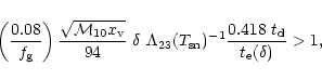
 from Appendix A, the condition of core
condensation C0, thus, can be expressed as
from Appendix A, the condition of core
condensation C0, thus, can be expressed as
![\begin{displaymath}\left (0.08 \over f_{\rm g} \right) {\sqrt{ {\cal M}_{10} x_{...
...rm v}} -{1 \over 2} \right]
\Lambda_{23}(T_{\rm v})^{-1} < 1.
\end{displaymath}](/articles/aa/full/2001/45/aa1409/img146.gif) |
(27) |
![\begin{figure}
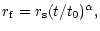
\par\includegraphics[width=8.8cm,clip]{MS1409f2.eps}\end{figure}](/articles/aa/full/2001/45/aa1409/Timg147.gif) |
Figure 2:
The dependence of the escape time of
the hot gas, in units of the dynamical time in the halo which is
defined as one-quarter oscillation period, on
 ,
the supernovae energy input in units of the halo binding energy. A factor of 10 in the heat input reduces the escape time, ,
by factor of 2. ,
the supernovae energy input in units of the halo binding energy. A factor of 10 in the heat input reduces the escape time, ,
by factor of 2. |
| Open with DEXTER |
After fragmentation and star formation, the gas is heated up and the
hot gas cools in a time,
 where
where
 is the temperature of the heated gas and
 .
Now, we need to compare this to the escape time, as defined in Eq. (11), when the condition C1 is satisfied or a quarter of the
oscillation period when the system is bound. Now,
.
Now, we need to compare this to the escape time, as defined in Eq. (11), when the condition C1 is satisfied or a quarter of the
oscillation period when the system is bound. Now,
 ,
is the mean energy of
a gas particle in the system and is zero when the escape velocity
equals the critical velocity. Using the potential for an isothermal
sphere that is truncated at ,
,
is the mean energy of
a gas particle in the system and is zero when the escape velocity
equals the critical velocity. Using the potential for an isothermal
sphere that is truncated at ,
 ,
and
,
and
 ,
we obtain
,
we obtain
which is valid for  ,
for which the supernova heat input,
,
is such that the resulting mean energy of the particles is
positive. These particles can escape only if the cooling time is
longer than the escape time. The escape time,
,
for which the supernova heat input,
,
is such that the resulting mean energy of the particles is
positive. These particles can escape only if the cooling time is
longer than the escape time. The escape time,
 ,
is a
slowly decreasing function and is of order
(See Fig. 2). For
,
is a
slowly decreasing function and is of order
(See Fig. 2). For  ,
the gas remains bound and only the condition of core condensation, C0, applies. Hence, the condition C2,
,
the gas remains bound and only the condition of core condensation, C0, applies. Hence, the condition C2,
 ,
can be expressed as
,
can be expressed as
 |
(29) |
where the effective dynamical timescale at  is taken to be
and
is taken to be
and
 ,
so that the curve C2 is continuous with C0.
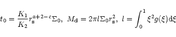
This is seen in the cooling diagram, presented in Fig. 3,
where the number density of hydrogen in the halo,
,
so that the curve C2 is continuous with C0.
This is seen in the cooling diagram, presented in Fig. 3,
where the number density of hydrogen in the halo,
 ,
is plotted against the virial temperature,
,
is plotted against the virial temperature,
 and shows the curves given by C0, the lower curve, C1, the
vertical line, and C2 which is the upper curve in the region to the
left of C1. The cosmological parameters were set to
and shows the curves given by C0, the lower curve, C1, the
vertical line, and C2 which is the upper curve in the region to the
left of C1. The cosmological parameters were set to
 ,
and
,
and
 and the halo parameters were chosen to be
 ,
and
,
and
 .
The shaded region
indicates the halos that have collapsed but star formation has induced
gas loss and they ultimately resulted in gas poor systems. The halos
above this region retain the gas that could form the massive central
black holes.
.
The shaded region
indicates the halos that have collapsed but star formation has induced
gas loss and they ultimately resulted in gas poor systems. The halos
above this region retain the gas that could form the massive central
black holes.
![\begin{figure}
\par\includegraphics[width=8.8cm,clip]{MS1409f3.eps}\end{figure}](/articles/aa/full/2001/45/aa1409/Timg168.gif) |
Figure 3:
The shaded region bounded by the constraints, C0, C1, and
C2 in the cooling diagram contains the halos that have cooled and
contracted to a radius of fragmentation; however, the supernovae
heated gas in these systems have escape times shorter than the
cooling time, resulting in gas-poor galaxies. The parameters chosen
here are
 ,
and ,
and
 .
The halos
above C2 for
(on the left of C1) and above C0 for
can trap the gas and hence are the candidate hosts of central
massive objects. .
The halos
above C2 for
(on the left of C1) and above C0 for
can trap the gas and hence are the candidate hosts of central
massive objects. |
| Open with DEXTER |
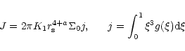
The corresponding range in mass for a given redshift is shown in Fig. 4, for the choices of the parameters,
,
the supernova efficiency, and
 ,
the fraction of baryons in stars. Clearly for large redshift, the mass range increases and this
is due to the deeper potential well which can retain the gas better.
There is a crucial question of whether all the gas is retained or if
some fraction is lost in a wind. A supernova efficiency in the halo of
,
the fraction of baryons in stars. Clearly for large redshift, the mass range increases and this
is due to the deeper potential well which can retain the gas better.
There is a crucial question of whether all the gas is retained or if
some fraction is lost in a wind. A supernova efficiency in the halo of
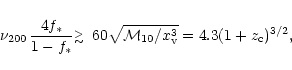 |
(30) |
from Eq. (29), would be required to drive winds that would result
in mass loss and this is considerably more than the corresponding estimates in our galaxy, for
 .
.
![\begin{figure}
\par\includegraphics[width=8.8cm,clip]{MS1409f4.eps}\end{figure}](/articles/aa/full/2001/45/aa1409/Timg172.gif) |
Figure 4:
The halos in the shaded region in the
 space
can trap the gas; the parameters chosen are
space
can trap the gas; the parameters chosen are
 ,
and ,
and
 . . |
| Open with DEXTER |
If the stars form after the disk forms, the cooling rate in the disk
would be given by
 |
(31) |
and the cooling time would reduce by a factor of a thousand
corresponding to enhanced density. Although only the cosmological
abundance of
![$[{\rm Fe/H}]=-4$](/articles/aa/full/2001/45/aa1409/img174.gif) was used, the supernovae explosions will also
enhance line cooling from metals injected into the medium; this would
reduce the cooling time estimated here.
was used, the supernovae explosions will also
enhance line cooling from metals injected into the medium; this would
reduce the cooling time estimated here.
3 Magnetization of the disk
In the large number of the halos which trap the gas as given by the
conditions C0-C2, a gaseous disk forms with a radial extent given in
Sect. 2.1. Further, it was seen in Sect. 2.3 that the
supernovae shells fill the core volume at the time of star formation,
and the small scale magnetic fields are dragged with the gas as it
settles into a the disk. Now, we consider the question of whether the
field strength is large enough to provide a significant viscous
stress. We take the gas to be initially dominated by the gravity of
the dark halo and assume the following logarithmic potential (Binney
& Tremaine 1987, Eqs. (2)-(54)) that obeys the flat rotation curve
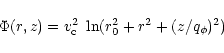 |
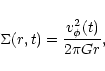
(32) |
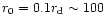
where r0 is the radius of a compact region,
 and
is defined in Eq. (22). If the vertical equilibrium was
a result of balance between vertical gradient in the total pressure,
and
is defined in Eq. (22). If the vertical equilibrium was
a result of balance between vertical gradient in the total pressure,
 (which represents a sum of magnetic and gas pressures and the density
scale height is H), and
(which represents a sum of magnetic and gas pressures and the density
scale height is H), and
 ,
we obtain
,
we obtain
 |
(33) |
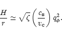
Assuming a dominant isothermal halo, we obtain the half-flaring angle
of the disk,
 |
(34) |
where
 ,
and the speed
of sound was taken to be
,
and the speed
of sound was taken to be
 cm s-1 for a temperature of 104 K,
where the cooling curve drops significantly.
cm s-1 for a temperature of 104 K,
where the cooling curve drops significantly.
The supernovae inject the medium with magnetic flux and next we
estimate the typical strength of the small scale field. The
calculation in Sect. 2.3 shows that the filling factor of the
shells in the total gas volume is nearly unity for a wide range in
density and therefore the supernovae hot gas fills the medium and
hence quasi-uniformly magnetizes it. The volume of the flared disk
works out to be
The Crab Nebula of size 0.8 pc (or volume 2 pc3) has
 G fields (see Sect. 7 for a discussion of supernova
field strengths). By freezing the flux in a Crab volume of 2 pc3 to
a volume occupied by one shell, the magnetic field strength in the
disk for
G fields (see Sect. 7 for a discussion of supernova
field strengths). By freezing the flux in a Crab volume of 2 pc3 to
a volume occupied by one shell, the magnetic field strength in the
disk for
 remnants
is
remnants
is
By choosing a typical set of values (
 )
the field strength turns out to be as high as
)
the field strength turns out to be as high as
 .
The mean number density of hydrogen atoms in the flared gaseous disk,
for ,
is given by
.
The mean number density of hydrogen atoms in the flared gaseous disk,
for ,
is given by
where (34) and (2) were used and the values of
and
 were taken. Outflows from O and B
stars could also magnetize the gas, and by using flux freezing we
estimate the field strength due to winds to be (Bisnovatyi-Kogan et al. 1973; Ruzmaikin et al. 1988)
were taken. Outflows from O and B
stars could also magnetize the gas, and by using flux freezing we
estimate the field strength due to winds to be (Bisnovatyi-Kogan et al. 1973; Ruzmaikin et al. 1988)
 |
(38) |
where the estimates of the density at the base of the wind,
 g cm-3 and the field at the surface of the star,
 are used. The field expelled by massive stars are unlikely
to pervade the volume, and the major contribution would be from
supernovae. Although the number of massive stars are of the same order
as the number of supernovae using the Salpeter IMF (estimated by integrating the mass range above
are used. The field expelled by massive stars are unlikely
to pervade the volume, and the major contribution would be from
supernovae. Although the number of massive stars are of the same order
as the number of supernovae using the Salpeter IMF (estimated by integrating the mass range above
 ;
see the footnote in Sect. 2.2), the smaller fluxes of the wind (
;
see the footnote in Sect. 2.2), the smaller fluxes of the wind (
 where
where  is the radius of the star) render the effective field strength to be
weak. The key point here, is that for typical values of the halo
parameters,
is the radius of the star) render the effective field strength to be
weak. The key point here, is that for typical values of the halo
parameters,
 is about 10-4-10-5G which is a factor of
10-100 higher than the value in our galaxy (
is about 10-4-10-5G which is a factor of
10-100 higher than the value in our galaxy (
 ) due to a smaller value of
 of the supernovae shells.
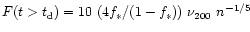
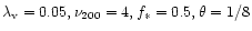
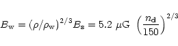
4 Accretion to a compact region
Here we consider different viscosity prescriptions, namely direct
magnetic stress, the phenomenological
viscosity (Shakura &
Sunyaev 1973) derived from magnetic fields, and angular momentum
transfer mediated by self-gravity induced instabilities, and calculate
the corresponding accretion timescales. The time dependent disk
accretion is described by the conservation of mass, radial momentum
(where all other forces except gravity are neglected, and
 and angular momentum
where
 is the surface density,
is the
gravitational potential and
is the surface density,
is the
gravitational potential and
 is the vertically integrated
stress. We take r0 as the inner radius of the disk flow and the
outer edge of the compact region while
is the vertically integrated
stress. We take r0 as the inner radius of the disk flow and the
outer edge of the compact region while
 |
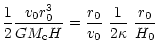
(42) |
By integrating Eq. (41), we obtain for steady flow
 |
(43) |
The viability of the various alternatives for the viscous stress can
be assessed by estimating the accretion rates. In the initial phase of
accretion the potential is dominated by the halo as calculated in Sect. 5, while in the later phase, self-gravity dominates and the resulting flow is calculated in Sect. 6.
4.1 Magnetic stress
We consider now the form of the stress tensor that is entirely due to
magnetic fields. We assume that the magnetic field injected is
largely in the form of small scale loops that are frozen into the
plasma. Further, we expect that the processes of compression and
advection preserves the form given by
 |
(44) |
that is likely to be valid for small scale fields in the
non-dissipative limit. The Lorentz force on the plasma is
![\begin{displaymath}({\vec J} \times {\vec B})_\phi ={1\over 4 \pi} ~ \left [{1 \...
...partial_{\rm r} (r B_\phi) + B_z \,\partial_z B_\phi \right ],
\end{displaymath}](/articles/aa/full/2001/45/aa1409/img216.gif) |
(45) |
where the first term on the right hand side is the local shear stress
and the second term is negligible in the initial phase (the vertical
average of small scale fields,
 ), but it could be important during a later phase of accretion
where magnetic braking can operate via built up, large scale Bz, by
angular momentum transfer to the parts external to the compact
region. Here, we take only the local shear stress
), but it could be important during a later phase of accretion
where magnetic braking can operate via built up, large scale Bz, by
angular momentum transfer to the parts external to the compact
region. Here, we take only the local shear stress 
 and this was assumed to be initially at sub-equipartition
levels as a thermal pressure (
and this was assumed to be initially at sub-equipartition
levels as a thermal pressure ( )
was used for calculating the
half-thickness of the initial disk in Eq. (34). One can verify
this through a consistency check by using the definition,
)
was used for calculating the
half-thickness of the initial disk in Eq. (34). One can verify
this through a consistency check by using the definition,
 ,
which determines the half-thickness,
,
which determines the half-thickness,
 from the condition of vertical equilibrium, (34),
 ,
from Eq. (36), and
,
from Eq. (36), and
 from Eq. (37). It follows that
 |
(46) |
and for a reasonable choice of parameters (
 )
this results in
)
this results in
 .
Low values of
.
Low values of
 ,
are typical for the
range of interest in the parameter space.
,
are typical for the
range of interest in the parameter space.
Next, we estimate the accretion time scale and hence the viability of
magnetic accretion in the steady limit. For typical values of the
parameters assumed here (
 )
the accretion rate turns out to be
)
the accretion rate turns out to be
using Eqs. (34), (22), (43). Taking the initial field
to be from supernovae expulsions (
 )
from Eq. (36),
this implies a time scale of magnetic accretion,
)
from Eq. (36),
this implies a time scale of magnetic accretion,
Having obtained this fast timescale to accrete
of gas, we
proceed to calculate the detailed form of
 .
The
thickness of the disk is given by Eq. (34), the balance of the
total pressure gradient and vertical gradient of the background
potential. Combining Eqs. (34), (44), and
.
The
thickness of the disk is given by Eq. (34), the balance of the
total pressure gradient and vertical gradient of the background
potential. Combining Eqs. (34), (44), and
 ,
we obtain
,
we obtain
 |
(49) |
where
 is the flaring angle
of the full thickness of the disk. Initially, the magnetic pressure is
lower than the thermal pressure but as the matter sinks into a compact
region the magnetic pressure is expected to dominate the vertical
pressure gradient.
is the flaring angle
of the full thickness of the disk. Initially, the magnetic pressure is
lower than the thermal pressure but as the matter sinks into a compact
region the magnetic pressure is expected to dominate the vertical
pressure gradient.
4.2
viscosity
If a small scale dynamo operates quickly (Kasantsev 1967; Kulsrud &
Anderson 1992) then it will saturate near equipartition values (as is
well known from simulations - Hawley et al. 1995 and
references therein) and an appropriate form of the stress can be
described in terms of a prescription of the form
 ,
where
,
where
 is the total pressure,
which is proportional to the gas pressure at equipartition. The
accretion time scale is expected to be similar to the one obtained
earlier. The dependence on the halo parameters can be expressed in
the isothermal limit as
is the total pressure,
which is proportional to the gas pressure at equipartition. The
accretion time scale is expected to be similar to the one obtained
earlier. The dependence on the halo parameters can be expressed in
the isothermal limit as
Note that, although we use a direct magnetic stress in our
calculations, we record for comparison, the detailed form of the
prescription in Appendix B.
4.3 Gravitational instabilities
Cold, thin rotating discs are known to be unstable and the basic
stability criteria was provided by Toomre (1964). For a uniformly
rotating isothermal disk (Goldreich
& Lynden-Bell 1965) the criteria for local stability is given by
 |
(51) |
We find that
 |
(52) |
where the values (
 )
were assumed. So the
disk is unstable to gravitational instabilities and it is possible for
angular momentum transport to occur through this process. Lin &
Pringle (1987) estimate an effective kinematic viscosity for
gravitational instability from
)
were assumed. So the
disk is unstable to gravitational instabilities and it is possible for
angular momentum transport to occur through this process. Lin &
Pringle (1987) estimate an effective kinematic viscosity for
gravitational instability from
 ,
where the
critical shearing length,
,
where the
critical shearing length,
 was taken to be
the maximum possible size for the instability. Here we make a more
conservative estimate by introducing the parameter,
was taken to be
the maximum possible size for the instability. Here we make a more
conservative estimate by introducing the parameter,
 ,
into the stress given by
,
into the stress given by
 |
(53) |
The corresponding timescale of accretion is
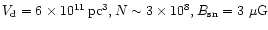
5 Self-similar evolution of the disk in a background potential
Having demonstrated that the time scales of accretion are quite fast,
we now proceed to calculate a detailed model of self-similar evolution
of a disk from the diffusion equation obtained from the conservation
laws (39-41)
![\begin{displaymath}\partial_{\rm t} \Sigma = {1 \over r} \partial_{\rm r} \left ...
...2 \omega)}
\partial_{\rm r}[r^2
\Pi_{{\rm r} \phi}] \right),
\end{displaymath}](/articles/aa/full/2001/45/aa1409/img258.gif) |
(55) |
where the viscous stress can be parameterized as
 and in addition the rotation law is assumed to be of the
form
and in addition the rotation law is assumed to be of the
form
 .
This very useful formulation of a self-similar
form is due to Pringle (1981) but only particular analytic solutions
to the diffusion equation has been reported for the specific cases of
(
a=-3/2, b=c=3; Lin & Pringle 1987) in the context of accretion of
a protostellar disk onto a point mass via gravitational instabilities
and (
a=-3/2, b=5/3, c=-1/2; Cannizzo et al. 1990 (CLG), see
Appendix B of this paper) in the context of disk accretion of a tidally
disrupted star onto a massive black hole. Note that in CLG, the
scaling law for the viscous stress by the closure of the conditions of
local dissipation in an alpha disk in a Kepler potential and vertical
equilibrium. Here, an analytic solution to the general problem of the
type (
.
This very useful formulation of a self-similar
form is due to Pringle (1981) but only particular analytic solutions
to the diffusion equation has been reported for the specific cases of
(
a=-3/2, b=c=3; Lin & Pringle 1987) in the context of accretion of
a protostellar disk onto a point mass via gravitational instabilities
and (
a=-3/2, b=5/3, c=-1/2; Cannizzo et al. 1990 (CLG), see
Appendix B of this paper) in the context of disk accretion of a tidally
disrupted star onto a massive black hole. Note that in CLG, the
scaling law for the viscous stress by the closure of the conditions of
local dissipation in an alpha disk in a Kepler potential and vertical
equilibrium. Here, an analytic solution to the general problem of the
type (
 )
is presented so that possible viscosity mechanisms discussed
earlier and expressible in this way, can be explored within the same
formulation. In the magnetic case given below, the viscosity scaling
is due a magnetic stress, the flux-freezing condition and vertical
equilibrium in a cold disk in the background halo potential. A
solution for an alpha disk with local dissipation with a general
rotation law is provided in Appendix B. The general solution
presented below has a larger utility in contexts other than one
considered here.
)
is presented so that possible viscosity mechanisms discussed
earlier and expressible in this way, can be explored within the same
formulation. In the magnetic case given below, the viscosity scaling
is due a magnetic stress, the flux-freezing condition and vertical
equilibrium in a cold disk in the background halo potential. A
solution for an alpha disk with local dissipation with a general
rotation law is provided in Appendix B. The general solution
presented below has a larger utility in contexts other than one
considered here.
If b=1, the equation is linear and the general solution is easily
found. Proceeding generally, under the assumptions of self-similarity
for ( ), one may write the the surface density in the
following form
), one may write the the surface density in the
following form
 |
|
 |
(56) |
where
 ,
and
,
and  is the associated radius scale. We
set the constants
is the associated radius scale. We
set the constants
 |
(57) |
where  is the initial disk mass. Here we seek a particular
solution when there is no external torque, which implies the total
angular momentum, J, of the disk is a constant. Using the scaling
relations above that are implicit in Eq. (55) and
is the initial disk mass. Here we seek a particular
solution when there is no external torque, which implies the total
angular momentum, J, of the disk is a constant. Using the scaling
relations above that are implicit in Eq. (55) and
 |
(58) |
it follows that
 and
and
 .
At this point we note that the disk edge travels outward if
2+c < b (4+a). Substituting into the form for the surface density,
as given in (56), and simplifying (55), we obtain the
following ordinary differential equation,
.
At this point we note that the disk edge travels outward if
2+c < b (4+a). Substituting into the form for the surface density,
as given in (56), and simplifying (55), we obtain the
following ordinary differential equation,
 |
(59) |
After some algebraic transformations, one can integrate it once to
obtain
 |
(60) |
Now, we apply the boundary condition that the density vanishes at the
disk edge, ie.,
 |
|
|
(61) |
Moreover, if b >1, which is the case for the examples considered
here, then c1=0. By rearranging terms and integrating, we obtain
the following solution
 |
(62) |
The time constant can be evaluated with
 to be
to be
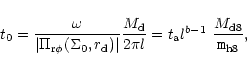 |
(63) |
where  is the accretion time scale calculated in Sect. 4.1 and Sect. 4.3 in the steady case using
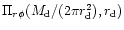 .
The rate at which mass sinks into the center is given by
.
The rate at which mass sinks into the center is given by
![\begin{displaymath}M_{\rm c}(t)= M_{\rm d} \left [1- \left ({t \over t_0}\right)^{-(a+2)\alpha}
\right].
\end{displaymath}](/articles/aa/full/2001/45/aa1409/img280.gif) |
(64) |
The accretion time scale which is the time that transpires when a
fraction
 of the disk mass falls in is given by
where
represents the timescales
 or
or  ,
and
indicates that the estimates derived earlier are modified by geometric
factors. Now we consider the particular case of magnetic accretion
(
,
and
indicates that the estimates derived earlier are modified by geometric
factors. Now we consider the particular case of magnetic accretion
(
 ,
see Sect. 4.1 where the value of
,
see Sect. 4.1 where the value of  is chosen for a
typical case where the disk mass,
is chosen for a
typical case where the disk mass,
 ,
and
,
and
 )
which has
the solution
)
which has
the solution
Similarly, the accretion due to gravitational instabilities (
 ,
,
and
,
see Sect. 4.3) has the solution
,
,
and
,
see Sect. 4.3) has the solution
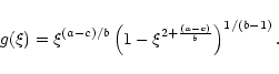
The disk structure of these solutions are shown in Fig. 5.
![\begin{figure}
\par\includegraphics[width=8.8cm,clip]{MS1409f5.eps}\end{figure}](/articles/aa/full/2001/45/aa1409/Timg298.gif) |
Figure 5:
The structure  of the
self-similar disk,
of the
self-similar disk,
 where
where
 .
The magnetic solution, .
The magnetic solution,
![$g_{\rm m}(\xi )=\xi ^{-1/2} \left [1-\xi ^{3/2}\right ]^3$](/articles/aa/full/2001/45/aa1409/img19.gif) is shown by a
solidline, and the solution of the disk with gravitational viscosity,
is shown by a
solidline, and the solution of the disk with gravitational viscosity,
![$g_{\rm g}(\xi )=\xi ^{-1} \left [1-\xi \right ]^{1/2}$](/articles/aa/full/2001/45/aa1409/img20.gif) ,
is shown by a dashed line. ,
is shown by a dashed line. |
| Open with DEXTER |
The self-similar solutions of this kind to (55) are known to
develop at large times in numerical simulations with a variety of
initial conditions (Lin & Pringle 1981).
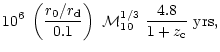
Now we determine the regime in parameter space where the halo dominated flow can occur. This is given by the condition that at t=t0 and
 ,
the halo dominates self-gravity or
,
the halo dominates self-gravity or
| |
|
 |
|
| |
|
 |
(68) |
where
is the circular velocity due to the halo alone, the disk
potential was expressed as a Bessel transform of the surface density
and  are the zeros of J0. The collapse factor
 from Sect. 2.1,
 by definition, leading to
 |
(69) |
For the solution (66), the magnetic case, the RHS of the
above equation works out to be 0.44 and for the gravitational
instability case, the solution (67), the corresponding
value is 0.46. Hence this condition can be written as
 |
(70) |
where k1=0.5 for a truncated isothermal sphere was used. For a
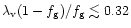
reasonable range in the parameters (
 -0.1,
-0.1,
 -0.08) the above condition holds good (
 is in the range 1-4); as a result, the initial accretion flow is
expected to be halo dominated. As the mass accretes into the center,
the spin deviates from
is in the range 1-4); as a result, the initial accretion flow is
expected to be halo dominated. As the mass accretes into the center,
the spin deviates from
 and gradually
increases. The self-similar solutions are valid only up to a point
beyond which the self-gravity due the disk and the central mass
dominates the potential. The time of transition to a self-gravitating
flow can be estimated by seeking that
and gradually
increases. The self-similar solutions are valid only up to a point
beyond which the self-gravity due the disk and the central mass
dominates the potential. The time of transition to a self-gravitating
flow can be estimated by seeking that
 |
(71) |
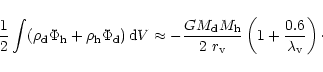
Now expressing time in terms of the
 in Eq. (64), we obtain after some algebra
 |
(72) |
where
 .
Clearly, this condition does not hold close to a
compact central region (defined by r<r0) where it is dominated by
the central mass. The solutions considered here are a good
approximation for the region beyond y=0.1 for
.
Clearly, this condition does not hold close to a
compact central region (defined by r<r0) where it is dominated by
the central mass. The solutions considered here are a good
approximation for the region beyond y=0.1 for
 and
provide a sufficiently accurate description (See Fig. 6).
and
provide a sufficiently accurate description (See Fig. 6).
![\begin{figure}
\par\includegraphics[width=8.8cm,clip]{MS1409f6.eps}\end{figure}](/articles/aa/full/2001/45/aa1409/Timg317.gif) |
Figure 6:
A density plot of the ratio of
self-gravity (disk and the central mass) to halo gravity defined as
 ,
showing the evolution of a magnetized disk
in the halo potential as the central mass increases to ,
showing the evolution of a magnetized disk
in the halo potential as the central mass increases to
 .
The horizontal axis is the in units of the
initial disk radius, .
The value of .
The horizontal axis is the in units of the
initial disk radius, .
The value of
 was chosen to be 3; the halo gravity (in units of
 )
dominates at radii outside a central region of )
dominates at radii outside a central region of
 .
This figure can be seen in color in the online version of the journal. .
This figure can be seen in color in the online version of the journal. |
| Open with DEXTER |
At large times, a Keplerian flow into the compact region can be
assumed to occur and one can use a self-similar flow again with
a=-3/2 and the corresponding magnetic stress taking into account
 in Eq. (34) (in combination with (44), and
)
leads to
in Eq. (34) (in combination with (44), and
)
leads to
 .
Similarly
.
Similarly
 from Eq. (53). However, the
estimate of the accretion timescale is not expected to be very
different from the one derived earlier. The key result is that about a
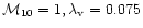
fraction, 0.3, of the disk mass can be transported into a central
region, which is a fraction, y= 0.1, of the initial disk radius
within the time given by the solutions (66). For typical
values, this implies that about
from Eq. (53). However, the
estimate of the accretion timescale is not expected to be very
different from the one derived earlier. The key result is that about a
fraction, 0.3, of the disk mass can be transported into a central
region, which is a fraction, y= 0.1, of the initial disk radius
within the time given by the solutions (66). For typical
values, this implies that about
 of gas sinks
into a
of gas sinks
into a
 pc region in a halo (with
 )
in a timescale of
)
in a timescale of
 yrs.
yrs.
6 Disk evolution in a self-gravitating regime
We now examine the evolution of the disk in a gravity field that is
entirely due to itself. This flow can occur after sufficient accretion
of mass into a compact region of radius r0; or, alternatively at
the time of the formation of the disk if the Eq. (70) is
not satisfied and
 .
The problem of
self-gravitating accretion flow is complicated by the coupling of
Poisson's equation to the momentum and continuity equations. Clearly,
its evolution has to be treated differently from the preceding case of
a prescribed background potential. A detailed model is deferred to a
work in preparation (Mangalam 2001); below, we consider a useful
simplified version of the problem by assuming a particular form of the
density distribution (see Field 1994).
.
The problem of
self-gravitating accretion flow is complicated by the coupling of
Poisson's equation to the momentum and continuity equations. Clearly,
its evolution has to be treated differently from the preceding case of
a prescribed background potential. A detailed model is deferred to a
work in preparation (Mangalam 2001); below, we consider a useful
simplified version of the problem by assuming a particular form of the
density distribution (see Field 1994).
We assume a Mestel (1963) disk where the self-consistent density
distribution with potential is entirely due to self-gravity, is of the form
 |
(73) |
where the time dependence appears only in the rotational
velocity. This is a an interesting disk which is self-consistent,
taking into account the most relevant physics. Taking
 |
(74) |
where
 ,
and
,
and  is the mass out to r0. We see
that by assuming a self-similar evolution of the disk, the mass out to
a given x should be independent of t and hence it follows that
is the mass out to r0. We see
that by assuming a self-similar evolution of the disk, the mass out to
a given x should be independent of t and hence it follows that
 |
(75) |
where
 .
From the continuity equation,
.
From the continuity equation,
 |
(76) |
we find
 |
(77) |
Substituting this and the self-similar forms given above into the
angular momentum equation,
we obtain
 |
(79) |
which is independent of x. So far no specific viscosity
mechanism has been invoked - the form of
above is
necessitated by the prescription of a Mestel disk. If a magnetic
stress is assumed and
 ,
where
,
where
 is a factor of order unity and B is given by the vertical
balance of magnetic pressure and gravity,
is a factor of order unity and B is given by the vertical
balance of magnetic pressure and gravity,
 .
It follows that the half thickness,
.
It follows that the half thickness,
 ,
and can be expressed as
,
and can be expressed as
 .
Furthermore, from the flux-freezing condition,
.
Furthermore, from the flux-freezing condition,
![$B
\propto \left [r^2 H \right]_{x=1}^{2/3}$](/articles/aa/full/2001/45/aa1409/img344.gif) ,
it is seen that p=-2. Equating the form
of
from Eq. (79) to a magnetic stress,
,
it is seen that p=-2. Equating the form
of
from Eq. (79) to a magnetic stress,
 ,
and writing (after taking
)
,
and writing (after taking
)
we see that
 |
(81) |
which leads to the solution
 |
(82) |
where  was taken as the initial condition. So the disk
spins up rapidly and shrinks to a smaller radius. Clearly, the
solution is no longer valid when it is relativistic. The self-similar
collapse of the compact region is only a sketch but nevertheless the
collapse timescale,
was taken as the initial condition. So the disk
spins up rapidly and shrinks to a smaller radius. Clearly, the
solution is no longer valid when it is relativistic. The self-similar
collapse of the compact region is only a sketch but nevertheless the
collapse timescale,  ,
suggests that formation of a black hole is
extremely rapid (106 yrs).
,
suggests that formation of a black hole is
extremely rapid (106 yrs).
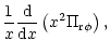
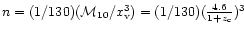
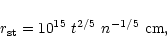
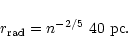
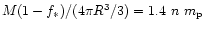
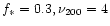
7 Summary of the results and discussion
We summarize our results as follows:
- 1.
- We considered star formation and supernovae feedback on the remaining
gas in the halo based on the framework of DS. We include a new and
necessary condition C2, namely that escape time for the hot gas be
shorter than the cooling time and find that the condition for gas loss
can be expressed by Eqs. (27), (23), (29) which is
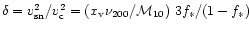
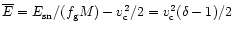
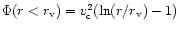
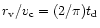
depicted in Fig. 3. For a typical choice of
and
,
Fig. 4 shows the allowed range for Halo mass in terms of
redshift. There is a sharp decline in the allowed range beyond
collapse redshifts of
 ,
as the potential wells formed at
earlier epochs are deeper and trap the gas better.
,
as the potential wells formed at
earlier epochs are deeper and trap the gas better.
- 2.
- It was seen in Sect. 2.3 that the hot gas from supernovae has a
filling factor of nearly unity and hence the small-scale magnetic
fields occupy the disk. It was shown in Sect. 3 the field
strength is significant (10-100
 G), based on typical values of
supernova efficiency, ,
and star fraction, .
G), based on typical values of
supernova efficiency, ,
and star fraction, .
- 3.
- In Sect. 4, we examined magnetic stress and viscosity due
to self-gravity induced instabilities that would operate in a
collapsed disk. The accretion timescales were estimated for a direct
magnetic stress, Eq. (48), an
prescription, Eq. (50), and self-gravity, Eq. (54), in terms of halo parameters
 and star formation parameters
 .
The timescales are all short compared to the cosmic time.
.
The timescales are all short compared to the cosmic time.
- 4.
- A general solution for a self-similar and time dependent accretion
flow for a viscous stress of the form
 in a prescribed potential,
 ,
was obtained in
Sect. 5. This was applied to the specific cases of magnetic
accretion, Eq. (66) and and gravitational instabilities,
Eq. (67). The structure of the resulting disk is shown in Fig. 5 and the timescales are within geometric factors of their estimates.
The disk eventually becomes fully Keplerian. The condition of halo
dominated flow is given by Eq. (70) and the transition to a
self-gravitating flow is given by Eq. (72). This solution is
valid for dominant halos in the initial stages for the outer parts,
y>0.1, oustide a Keplerian compact region for up to time when a
fraction of the disk mass,
,
was obtained in
Sect. 5. This was applied to the specific cases of magnetic
accretion, Eq. (66) and and gravitational instabilities,
Eq. (67). The structure of the resulting disk is shown in Fig. 5 and the timescales are within geometric factors of their estimates.
The disk eventually becomes fully Keplerian. The condition of halo
dominated flow is given by Eq. (70) and the transition to a
self-gravitating flow is given by Eq. (72). This solution is
valid for dominant halos in the initial stages for the outer parts,
y>0.1, oustide a Keplerian compact region for up to time when a
fraction of the disk mass,
 ,
falls in (see Fig. 6).
,
falls in (see Fig. 6).
- 5.
- A self-gravitating Mestel disk that is spinning up as it is collapsing
self-similarly, is described in Sect. 6. We apply this to a
compact region where the pressure is assumed to be due to magnetic
fields. The time scale of collapse turns out to be the rotation time
of the outer radius, which is a few million years.
We now discuss some of the issues involved:
Supernovae feedback
In a pioneering work, DS, showed that with a model of protogalactic
gas in a halo reproduces the observed relations very well with an
initial CDM model. Further, the condition for gas loss was given by
the condition that the energy input from supernovae is more than the
binding energy, C1 and the cooling condition for gas contraction and
star formation. In this work, we specify an additional necessary
condition, C2, that the escape time be shorter than the cooling
time. As indicated in Fig. 3, this restricts the gas loss to
the halos in the shaded region. The exact shape and location of the
region is subject to the choice of parameters (
 ), but the
key point made here is that the entire region to the left of C1 cannot
be considered as a gas loss zone, even if heating by background UV
photons were included. It is worth investigating this question in more
detail by simulations that include the hydrodynamics and cooling of
the hot gas. Based on this study, one can conclude that most of the
dwarf galaxies involved efficient conversion of stars or high
efficiency of supernovae, since that would place curve C2, higher on
the cooling diagram accounting for the prediction of the location of
the dwarf galaxies made by DS. The constraints imposed here, however,
account for the presence of black hole systems on the left of C1 (and
above C2). It also explains a sharp decline in quasars at epochs
later than z=2.
), but the
key point made here is that the entire region to the left of C1 cannot
be considered as a gas loss zone, even if heating by background UV
photons were included. It is worth investigating this question in more
detail by simulations that include the hydrodynamics and cooling of
the hot gas. Based on this study, one can conclude that most of the
dwarf galaxies involved efficient conversion of stars or high
efficiency of supernovae, since that would place curve C2, higher on
the cooling diagram accounting for the prediction of the location of
the dwarf galaxies made by DS. The constraints imposed here, however,
account for the presence of black hole systems on the left of C1 (and
above C2). It also explains a sharp decline in quasars at epochs
later than z=2.
Magnetic field strength in supernovae shells
In estimating the field strength
in Sect. 3, all the
shells were assumed to have 10-4 G when they are young (size of
0.8 pc) and flux freezing was used to estimate the values at a given
size. This field has been measured in the Crab nebula and in other
young supernova remnants like Tycho, Kepler and Cas A, the field
strength in the shell is inferred to be 10-3-10-4 G (Strom &
Duin 1973; Henbest 1980; Anderson et al. 1991). Simulations by Jun & Norman (1996), show local turbulent amplification by Rayleigh-Taylor
and Helmholtz instabilities but claim overall sub-equipartition
strengths. An analysis of Cas A X-ray and radio surface brightness at
high resolution, show that there is a strong correlation, implying a
possible equipartition between the field (mG) and the hot gas
(Keohane et al. 1998). The field amplification can be from other sources as well. For example, the magnetic field in the Crab has been wound up in
the body of the nebula by the pulsar and the magnetic energy is a few
a percent of the spin energy (Rees & Gunn 1974). High resolution
simulations of a supernova including rotation and expanding in an
unmagnetized medium, which to our knowledge are unavailable, are best
suited to the answer the question of the initial field strength in the
disk. The small scale fields that are injected in the medium could be
amplified to saturation levels by a dynamo operating in the disk aided
by differential rotation and turbulent motion. Since this
amplification was not taken into account (no assumption other than
flux-freezing was made for the field evolution), the field strengths
derived from supernovae which is in the range 10-100 G, could be
an underestimate.
Large scale fields
Strong fields of a few G are estimated from Faraday rotation of
background QSOs by damped Ly
absorptions systems, which are
thought to be proto-galactic disks, as early as  ,
imposing
constraints on the kinematic dynamo (Kronberg et al. 1992). A primordial origin for the large scale field in galaxies has been speculated upon (Rees 1994; Ratra 1992 and references therein), but the field generated by these mechanisms is much smaller than the magnitude required for a primeveal hypothesis. Large-scale magnetic
fields in the galaxy are thought to be generated by a turbulent dynamo
from a weak seed field (10-19 G). But, it has been argued
that magnetic energy at small (eddy) scales builds up much faster (at
eddy turnover rates) than the mean field, so that the kinematic dynamo
shuts off before the large scale fields amplify to observed levels
(Kulsrud & Anderson 1992; Kasantsev 1967) if the initial seed is
weaker than 10-9 G. Subramanian (1998) argues, however, that the
fields are intermittent and do not fill the volume. The small scale
flux ropes are at saturated values but the mean energy density is at
sub-equipartition levels allowing the large scale field to grow to
equipartition strength, aided by ambipolar drift. This question is
still unresolved, but if the supernovae field can provide a fairly
strong seed field (
,
imposing
constraints on the kinematic dynamo (Kronberg et al. 1992). A primordial origin for the large scale field in galaxies has been speculated upon (Rees 1994; Ratra 1992 and references therein), but the field generated by these mechanisms is much smaller than the magnitude required for a primeveal hypothesis. Large-scale magnetic
fields in the galaxy are thought to be generated by a turbulent dynamo
from a weak seed field (10-19 G). But, it has been argued
that magnetic energy at small (eddy) scales builds up much faster (at
eddy turnover rates) than the mean field, so that the kinematic dynamo
shuts off before the large scale fields amplify to observed levels
(Kulsrud & Anderson 1992; Kasantsev 1967) if the initial seed is
weaker than 10-9 G. Subramanian (1998) argues, however, that the
fields are intermittent and do not fill the volume. The small scale
flux ropes are at saturated values but the mean energy density is at
sub-equipartition levels allowing the large scale field to grow to
equipartition strength, aided by ambipolar drift. This question is
still unresolved, but if the supernovae field can provide a fairly
strong seed field ( 10-9 G), then a kinematic dynamo can
operate to amplify the fields to
10-9 G), then a kinematic dynamo can
operate to amplify the fields to
 strengths in a galactic
disk. A sphere of radius L, encloses
strengths in a galactic
disk. A sphere of radius L, encloses
 remnants where
 is the size of a remnant. The rms value of the field at a
scale
is the size of a remnant. The rms value of the field at a
scale
 would be roughly
 .
At
the scale of the compact region, L=r0=100 pc, the large scale seed
field is of order 10-7 G.
.
At
the scale of the compact region, L=r0=100 pc, the large scale seed
field is of order 10-7 G.
Angular momentum transport
There is an angular momentum transport mechanism required to form a
seed mass in a central region and one for the compact central mass to
further collapse; the two schemes, in principle, can be
different. Loeb & Rasio (1994) concluded from hydrodynamic
simulations that fragmentation occurs halting a direct collapse to
relativistic scales and suggested that low spin systems could form
supermassive seeds of disk or star geometry which would contract under
radiative viscosity. The picture proposed here is that direct
magnetic stress or gravitational instabilities in the disk can
transport matter into a compact region on a dynamical timescale. The
scheme of gravitational instabilities hinges on
 in the disk
whereas the direct magnetic stress depends on the supernova efficiency
and field expulsion. The presence of high magnetic energy density from
MHD turbulence has been invoked to explain high velocity dispersions
of H I clouds in galactic disks (Sellwood & Balbus 1999).
in the disk
whereas the direct magnetic stress depends on the supernova efficiency
and field expulsion. The presence of high magnetic energy density from
MHD turbulence has been invoked to explain high velocity dispersions
of H I clouds in galactic disks (Sellwood & Balbus 1999).
Angular momentum in the inner region ( 1 pc) is likely to be
more complicated due to radiation pressure that would prevent
collapse. The model of self-gravitating magnetized collapse in Sect. 6 was illustrative of the timescale involved but a detailed model for the inner region that takes into account radiation pressure, radiative viscosity and evolution of the field is required. If dynamo
action takes place within the compact region (100 pc), the
exponentiation timescale in the linear regime will be of order
1 pc) is likely to be
more complicated due to radiation pressure that would prevent
collapse. The model of self-gravitating magnetized collapse in Sect. 6 was illustrative of the timescale involved but a detailed model for the inner region that takes into account radiation pressure, radiative viscosity and evolution of the field is required. If dynamo
action takes place within the compact region (100 pc), the
exponentiation timescale in the linear regime will be of order
 yrs. The residual large scale seed field
(10-7 G) from supernovae can be amplified to dynamical
values (mG) in 107 years and the e-folding timescale for magnetic
braking is
yrs. The residual large scale seed field
(10-7 G) from supernovae can be amplified to dynamical
values (mG) in 107 years and the e-folding timescale for magnetic
braking is
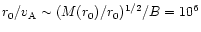 yrs corresponding
to this field strength.
yrs corresponding
to this field strength.
8 Conclusions
In this work, a semi-analytic model of quasar formation was attempted
which captures the essential details of star formation with supernovae
feedback and angular momentum transport via magnetic fields and
self-gravity. Based on the results in this work (as summarized in Sect. 7), and for the relevant range in parameter space, it is seen that a
cloud at z of 8 can collapse to form a gaseous disk in the dark halo by z of 4.8 and about 107-
of gas (which is 0.01-0.1 of the total disk mass) accretes into a
pc region in a fast timescale of 108 yrs. The magnetic stress from supernovae can be significant in the disk and
is preferred over other possibilities as observational evidence exists
for star formation, and large scale fields at .
The collapse
solutions do not hinge on the source of magnetic fields- SN or small
scale dynamo. The small scale dynamo needs a few rotation time scales
to build up and that could be significant - 108 yrs. The arguments
for SN fields are given in section Sect. 4.1; the strong
fields suggested can cause fast accretion rates instantly after the
disk forms. The field strength estimation relies only on flux freezing
arguments. Further, the alternative collapse solution using
gravitational instabilty is also given.
The solution to the non-linear diffusion equation presented in Sect. 5 can be applied in other contexts, e.g. protostellar disks. As a part of future work it is planned to investigate a detailed model of the inner region using a simulational approach, the impact of the restriction on the mass range of black hole hosts (
 )
by supernovae feedback on the details of the quasar luminosity function, dwarf galaxy formation, and the strength of the large scale seed field.
)
by supernovae feedback on the details of the quasar luminosity function, dwarf galaxy formation, and the strength of the large scale seed field.
Acknowledgements
I thank K. Subramanian for discussions. I thank the referee for helpful comments and suggestions.
Appendix A: Core condensation in halos
Here we calculate the change in gravitational potential energy from a
truncated isothermal halo to a truncated isothermal halo of stars and
dark matter containing an exponential gas disk. The final halo mass,
 is taken to be due to stars and dark matter, and
remaining mass is in the form of a gaseous disk with
is taken to be due to stars and dark matter, and
remaining mass is in the form of a gaseous disk with
 where
is the gas fraction. The initial
potential energy is given by
where
is the gas fraction. The initial
potential energy is given by
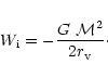 |
(A.1) |
The final potential energy is given by
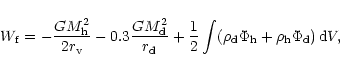 |
(A.2) |
where the first two term represents the self potential energies due a
truncated isothermal halo of size ,
and an exponential disk of
size ,
respectively, and the third term is due to the interaction
between them. The first part of the last term with (the disk surface
density
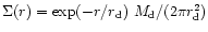 and
and
 )can be reduced to
 where the term involving
is
negligible in the range of interest for which
where the term involving
is
negligible in the range of interest for which
 .
The second part of the interaction term can be evaluated
with the disk potential expressed as a Bessel series in the region
.
The second part of the interaction term can be evaluated
with the disk potential expressed as a Bessel series in the region
 where
where
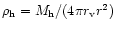 contributes. This term
works out to be
contributes. This term
works out to be
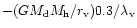 to a good
approximation, where the collapse factor,
to a good
approximation, where the collapse factor,
 ,
is in the range 10-20 (see Sect. 2.1). Combining the two we obtain
,
is in the range 10-20 (see Sect. 2.1). Combining the two we obtain
Finally, we obtain the change in gravitational potential energy
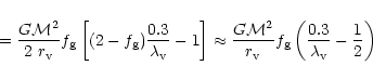 |
(A.3) |
which is bounded by
 .
.
Appendix B: Time-dependent evolution
of an alpha disk
Here we first consider a simple polytrope and then discuss the case of
a disk coupled with an local energy dissipation condition. By
assuming that the gas is a polytrope of index  ,
,
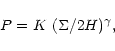 |
(B.1) |
and using the vertical equilibrium, Eq. (33), we obtain
In some applications it is appropriate to consider a disk with an
energy dissipation condition as has been done by Cannizzo et al. 1990 (CLG), for the case of disk accretion of a tidally distrupted star onto a massive black hole. Using the solution
presented in Sect. 5, we can generalize to a case of a rotational
law,
,
and viscous stress,
.
The viscous stress is given by
 |
(B.3) |
where T refers to the central temperature and P is the gas
pressure. Further, in the general prescription, the radiative flux is
matched to the viscous dissipation by
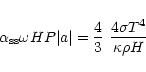 |
(B.4) |
where  is the Stefan-Boltzmann constant and
 is the opacity. This reduces to
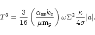 |
(B.5) |
Now, putting this back in Eq. (B.3), we obtain
This implies
b=5/3, c=a/3 for a constant .
For the case of a
Kepler potential we obtain the scaling (and opacity due to electron
scattering which is a constant) used in CLG (
a=-3/2, c=-1/2, b=5/3)
and their solution is given by Eq. (62) for these
indices. The case of a flat rotation law and opacity due to electron
scattering yields (
a=-1, b=5/3, c=-1/3). This solution can be easily
extended to more general opacities of the form
 ,
such as the Kramer's, and the appropriate solutions can be
easily found.
,
such as the Kramer's, and the appropriate solutions can be
easily found.
-
Anderson, M., Rudnick, L., Leppick, P., & Braun, R. 1991, ApJ, 373,
146
In the text
NASA ADS
-
Bahcall, J. N., & Soniera, R. M. 1980, ApJS, 44, 73
NASA ADS
-
Barnes, J., & Efsthasiou, G. 1987, ApJ, 319, 575
In the text
NASA ADS
-
Binney, J., & Tremaine, S. 1987, Galactic Dynamics (Princeton:
Princeton University Press)
In the text
-
Bisnovatyi-Kogan, G. S., Ruzmaikin, A. A., & Sunyaev, R. A. 1973,
SvA, 17, 137
In the text
NASA ADS
-
Blandford, R. D., & Rees, M. J. 1992, in Testing the AGN Paradigm,
ed. S. S. Holt, S. G. Neff, & C. M. Urry (New York: Am. Inst. Phys.), 3
In the text
-
Cannizzo, J. K., Lee, H. M., & Goodman, J. 1990, ApJ, 351, 38 (CLG)
In the text
NASA ADS
-
Chevalier, R. A. 1974, ApJ, 188, 501
In the text
NASA ADS
-
Dekel, A., & Silk, J. 1986, ApJ, 303, 39 (DS)
In the text
NASA ADS
-
Eisenstien, D. J., & Loeb, A. 1995, 443, 11
-
Ferrara, A., & Tolstoy, E. 2000, 313, 291
In the text
-
Ferrarese, L., & Merritt, D. 2000, ApJ, 539, L9
In the text
NASA ADS
-
Field, G. B. 1994, in Cosmical Magnetism, ed. D. Lynden-Bell (Cambridge:
Institute of Astronomy, Cambridge)
In the text
-
Ford, H. C., Harns, R. J., Tsvetarov, Z. I., et al. 1994, ApJ, 435, L27
In the text
NASA ADS
-
Gebhardt, K., Kormendy, J., Ho, L. C., et al. 2000, ApJ, 543, L5
In the text
NASA ADS
-
Goldreich, P., & Lynden-Bell, D. 1965, MNRAS, 130, 125
In the text
NASA ADS
-
Haenelt, M. G., & Rees, M. J. 1993, MNRAS, 263, 168
NASA ADS
-
Hamann, F., & Ferland, G. 1992, ApJ, 391, L53
In the text
NASA ADS
-
Hawley, J. F., Gammie, C. F., & Balbus, S. A. 1995, ApJ, 440, 742
In the text
NASA ADS
-
Heavens, A. F., & Peacock, J. A. 1988, MNRAS, 232, 339
In the text
NASA ADS
-
Henbest, S. N. 1980, MNRAS, 190, 833
In the text
NASA ADS
-
Jun, B.-I., & Norman, M. L. 1996, ApJ, 465, 800
In the text
NASA ADS
-
Kasantsev, A. P. 1968, Sov. Phys. - JETP, 26, 1031
-
Keohane, J. W., Gotthelf, E. V., & Petre, R. 1998, ApJ, 503, L175
In the text
NASA ADS
-
Kormendy, J., & Richstone, D. O. 1995, A&AR, 33, 581
In the text
-
Kronberg, P. P., Perry, J. J., & Zukowski, E. L. H. 1992, ApJ, 387,
528
In the text
NASA ADS
-
Kulsrud, R., & Anderson, S. W. 1992, ApJ, 396, 606
In the text
NASA ADS
-
Larson, R. B. 1974, MNRAS, 169, 229
In the text
NASA ADS
-
Lin, D. N. C., & Pringle, J. E. 1987, MNRAS, 607
In the text
-
Loeb, A., & Rasio, F. A. 1994, ApJ, 432, 52
In the text
NASA ADS
-
MacLow, M.-M., & Ferrara, A. 1999, 513, 142
-
Mangalam, A. 2001, A&A, in preparation
In the text
-
Mestel, L. 1963, MNRAS, 126, 553
In the text
NASA ADS
-
Miyoshi, M., Morar, J., Hermsteir, J., et al. 1995, Nature, 373, 127
In the text
NASA ADS
-
Natarajan, P. 1999, ApJ, 512, L105
In the text
NASA ADS
-
Padmanabhan, T., & Subramanian, K. 1992, BASI, 20, 1
In the text
NASA ADS
-
Padmanabhan, T. 1993, Structure Formation in the Universe (Cambridge:
Cambridge University Press)
In the text
-
Peebles, P. J. E. 1980, Large Scale Structure of the Universe (Princeton: Princeton University Press)
In the text
-
Pringle, J. E. 1981, A&AR, 19, 137
In the text
-
Ratra, B. 1992, ApJ, 391, L1
In the text
NASA ADS
-
Rees, M. J., & Gunn, J. E. 1974, MNRAS, 167, 1
In the text
NASA ADS
-
Rees, M. J., & Ostriker, J. P. 1977, MNRAS, 179, 451
In the text
-
Rees, M. J. 1984, A&AR, 22, 471
In the text
-
Rees, M. J. 1994, in Cosmical Magnetism, ed. D. Lynden-Bell (London:
Kluwer)
In the text
-
Ruzmaikin, A. A., Shukorov, A. M., & Sokoloff, D. D. 1988, Magnetic
Fields of Galaxies (Dordrecht: Kluwer)
In the text
-
Shakura, N. J., & Sunyaev, R. A. 1973, A&A, 24, 337
In the text
NASA ADS
-
Shapiro, S. L., & Teukolsky, S. A. 1983, Black Holes, White Dwarfs and
Neutron Stars (New York: Wiley)
-
Shlosman, I., Begelman, M. C., & Frank, J. 1990, Nature, 345, 679
In the text
NASA ADS
-
Silk, J. I. 1977, ApJ, 211, 638
In the text
NASA ADS
-
Silk, J. I., & Rees, M. J. 1998, A&A, 331, L1
In the text
NASA ADS
-
Sellwood, J. A., & Moore, E. M. 1999, ApJ, 510, 125
NASA ADS
-
Sellwood, J. A., & Balbus, S. A. 1999, ApJ, 511, 660
In the text
NASA ADS
-
Subramanian, K. 1998, MNRAS, 294, 718
In the text
NASA ADS
-
Sutherland, R., & Dopita, M. A. 1993, ApJS, 88, 253
In the text
NASA ADS
-
Strom, R. G., & Duin, R. M. 1973, A&A, 25, 351
In the text
NASA ADS
-
Spitzer, L. 1978, Physical Processes in the Interstellar Medium (New
York: Wiley)
In the text
-
Toomre, A. 1964, ApJ, 139, 1217
In the text
NASA ADS
-
Wandel, A. 1999, ApJ, 519, L39
In the text
NASA ADS
-
White, S. D. M., & Rees, M. J. 1978, MNRAS, 183, 341
NASA ADS
Copyright ESO 2001
![\begin{figure}
\par\includegraphics[width=8.8cm,clip]{MS1409f1.eps}\end{figure}](/articles/aa/full/2001/45/aa1409/img45.gif)
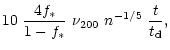

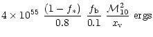
![\begin{figure}
\par\includegraphics[width=8.8cm,clip]{MS1409f2.eps}\end{figure}](/articles/aa/full/2001/45/aa1409/img147.gif)
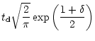
![$\displaystyle \times \left [ 1 - {\rm Erf}\left
( \sqrt{\frac{1 + \delta}{2}} \right ) \right ] ~ \delta \geq 1$](/articles/aa/full/2001/45/aa1409/img156.gif)
![\begin{figure}
\par\includegraphics[width=8.8cm,clip]{MS1409f3.eps}\end{figure}](/articles/aa/full/2001/45/aa1409/img168.gif)
![\begin{figure}
\par\includegraphics[width=8.8cm,clip]{MS1409f4.eps}\end{figure}](/articles/aa/full/2001/45/aa1409/img172.gif)
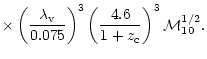
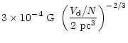
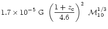
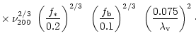
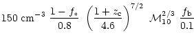
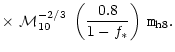
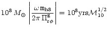
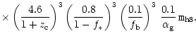
![\begin{figure}
\par\includegraphics[width=8.8cm,clip]{MS1409f5.eps}\end{figure}](/articles/aa/full/2001/45/aa1409/img298.gif)
![\begin{displaymath}(1-\epsilon)^3 {j y \over l^2}
\left [
\sum_n
\alpha_n^2 J_1...
...0^1 J_0(\xi \alpha_n) g(\xi) \xi
{\rm d}\xi \right] \nonumber
\end{displaymath}](/articles/aa/full/2001/45/aa1409/img313.gif)
![\begin{figure}
\par\includegraphics[width=8.8cm,clip]{MS1409f6.eps}\end{figure}](/articles/aa/full/2001/45/aa1409/img317.gif)