 |
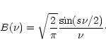
Figure 1: Noise spectra of bolometer signal (upper curve) and amplifier (lower curve). |
| Open with DEXTER | |
A&A 379, 735-739 (2001)
DOI: 10.1051/0004-6361:20011227
L. A. Reichertz - B. Weferling - W. Esch - E. Kreysa
Max-Planck-Institut für Radioastronomie (MPIfR), Auf dem Hügel 69, 53121 Bonn, Germany
Received 22 June 2001 / Accepted 30 August 2001
Abstract
Fastscanning is a new observing technique for millimeter and submillimeter
astronomy from ground based telescopes. The atmosphere is eliminated by taking advantage
of detector arrays. Instead of wobbling the secondary mirror with a fixed frequency
of a few Hz to filter the atmospheric contribution, we sample the
detector outputs at a much higher rate without a modulation by the
secondary mirror.
The atmospheric contribution is then removed later in the offline
data reduction by correlation analysis between the detector pixels.
In order to satisfy the AC requirement of the amplifiers in the absence of modulation,
the telescope scans fast to convert the spatial frequencies of the sky
into the detector frequency band. The acquired AC signals are then deconvolved
with the corresponding filter function in order to reconstruct quasi-DC signals.
This article describes the technique
of this new method and shows simulations and preliminary test results.
Key words: methods: observational - techniques: photometric - atmospheric effects
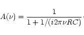
Astronomical observations from ground based telescopes in the (sub)millimeter wavelength regime are strongly compromised by fluctuations of the atmospheric emission. This is especially true for broadband measurements with sensitive detectors like bolometers. In order to subtract the atmospheric contribution from the measurement, dual beam techniques have been used for many years. A common method is to use a chopping (wobbling) secondary mirror which alternatively points the beam to two adjacent positions on the sky. After phase sensitive detection, spatial and temporal emission fluctuations should cancel, at least to first order. Since the introduction of the EKH algorithm (Emerson et al. 1979) this technique is applied even to extended sources which are many times larger in angular extent than the separation of the beams. Invented originally for single pixel detectors, this method is used today even with large arrays of detectors.
Despite the great success of this technique, a wobbling secondary mirror has some major disadvantages: A fast, precisely moving mirror is quite a technical challenge, particularly for large telescopes. Therefore, actually only low modulation frequencies (e.g. 2 Hz at the 30 m Millimeter Radio Telescope (MRT)) are possible. This limits the scan velocity in mapping modes and makes it difficult to achieve the required noise limit in readout electronics, as will be described in Sect. 2. The mechanics of a wobbling mirror usually allows only a certain direction of the movement which restricts the coordinate system of the observing modes. It is also a source of vibrations that can lead to microphonics in the signals of highly sensitive bolometers. Small asymmetries in the wobbling can lead to large offsets, due to different optical paths for each beam. Last but not least, a wobbling secondary mirror is not available on every telescope where continuum observations are of interest. In this paper we present a new mapping technique where a wobbling secondary mirror is no longer necessary.
The realisation of this quite simple idea has non-trivial
consequences for the data acquisition principles and readout electronics.
This will be explained in the following.
Along with the creation of a dual beam, the wobbling mirror has a second
function: The signal of interest is modulated at the wobbling frequency
and this allows the application of a phase-sensitive demodulation (Lock-In)
technique. Readout electronics for bolometers are therefore optimized
for low frequency AC signals.
| |
Figure 1: Noise spectra of bolometer signal (upper curve) and amplifier (lower curve). |
| Open with DEXTER | |
 |
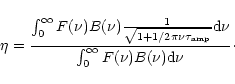
Figure 2: a) Amplitude and b) phase of the complex bolometer filter function. |
| Open with DEXTER | |
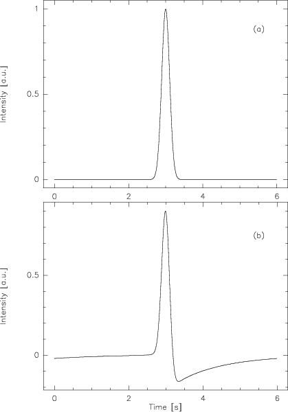 |
Figure 3: Simulated point source scan: a) before and b) after convolution with the filter function. |
| Open with DEXTER | |
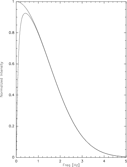 |
Figure 4: Point source scan in frequency space: before (upper curve) and after (lower curve) multiplication with the filter function. |
| Open with DEXTER | |
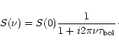
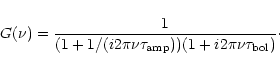
The responsivity of a bolometer is a function of its heat capacity ![]() and the thermal conductance
and the thermal conductance ![]() of the thermal link.
Although these are rather complicated functions of temperature and other
parmeters, in a first order approximation for small signals they can
be regarded as constant and the bolometer can be described in a
simple model with an effective thermal time constant (e.g. Richards 1994)
of the thermal link.
Although these are rather complicated functions of temperature and other
parmeters, in a first order approximation for small signals they can
be regarded as constant and the bolometer can be described in a
simple model with an effective thermal time constant (e.g. Richards 1994)
 |
(2) |
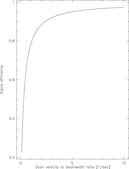 |
Figure 5: Signal efficiency as a function of the scan velocity to beamwidth ratio for a scan on a point source. |
| Open with DEXTER | |
In order to study the expected signals, computer simulations were performed with several parameter sets. Figure 3 shows an example with realistic assumptions. In this simulation a 30 m telescope scan across a point source was assumed. At 250 GHz, the beam has a beamwidth of about 10.5 arcsec FWHM. With a scanning velocity of 40 arcsec/s, a scan length of 240 arcsec and the assumption of a Gaussian beam, this results in an input signal for the bolometers as shown in Fig. 3a. The convolution of this signal with the bolometer filter function is illustrated in the following. Figure 4 shows the frequency spectrum of the original signal and after multiplication with Eq. (4). The resulting signal after the transformation back to the time space is displayed in Fig. 3b. This is the signal we expect to acquire in the absence of noise. To get back to the original Gaussian shape of the beam on a point source, the measured data need to be deconvolved by the inverse procedure.
Figure 4 indicates that even for high scanning velocities and the smallest
possible structure, namely a point source, only relatively low signal
frequencies are generated. That means, for bolometers with a time constant
like the ones in MAMBO, the effect of the bolometer response is negligible
in the analysis of the convolution. Furthermore, it shows the signal losses
which occur due to the attenuation of the lowest frequencies.
The ratio of the integral values for both spectra is a measure of the efficiency
and can be calculated as a function of the three parameters
scanning velocity v, beamwidth d and source extension s.
We begin with the input signal in Fig. 3a
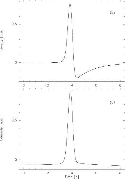 |
Figure 6: Experimental result of a scan on Saturn: a) raw signal of the center channel b) after the deconvolution. |
| Open with DEXTER | |
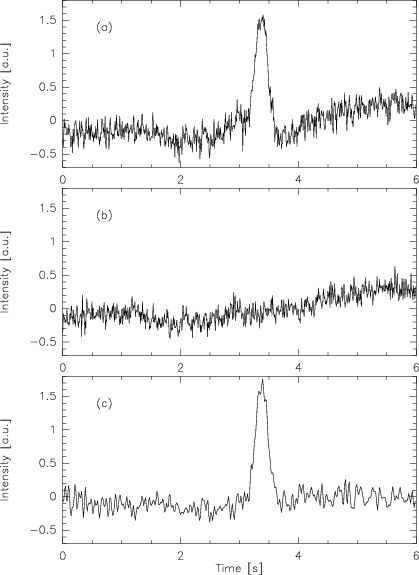 |
Figure 7: Experimental result of a scan on a 7 Jy point source: signal of the center array channel after removing the atmospheric noise by substracting the signal of another channel, a) raw signal of the center channel b) array channel without source, c) difference including the deconvolution. |
| Open with DEXTER | |
The following experimental setup was used to test the method at the 30 m MRT with real data. A fast readout of the 37 channels of the MAMBO array was necessary. We chose a commercial off-the-shelf 16 bit A/D converter module with 64 multiplexed input channels that was plugged into the PCI bus of a PC. To avoid excess noise due to aliasing errors, we included anti-aliasing filters between the bolometer amplifier and the A/D converter. These filters modified the bolometer filter function in such a way that the roll-off for higher frequencies became steeper. After inclusion of the filters it was checked that the bolometer noise was well sampled at the frequency of 125 Hz. During the observations the data of each bolometer channel, sampled at a rate of 125 Hz, were streamed to a local harddisk of the PC together with an absolute timestamp.
Figure 6 shows the result of a scan on Saturn obtained at the 30 m telescope. The scan duration was 8 s with a scan velocity of 40 arcsec/s. Saturn had a 250 GHz flux of 635 Jy at that time. In this figure the signal of the central array channel is shown. Figure 6a shows the raw signal without deconvolving the data by the bolometer filter function and Fig. 6b shows the result after the raw data were deconvolved. One can see that the distortion of the signal due to the filter function is removed, the original signal from the telescope beam on a point-like source is obtained as expected from the simulations.
In the next example the measurement of the source K3-50A with 250 GHz flux of 7 Jy is presented. This weaker source shows the effect of the atmospheric noise as a variable baseline (Fig. 7a). A neighbouring channel of the array in Fig. 7b that did not scan the source at the same time has the same structure in the baseline and demonstrates the strong correlation of the sky emission in different channels. This signal can be used to remove the atmospheric contribution in Fig. 7a. The result is shown in Fig. 7c. Restoring the original signal by the deconvolving procedure allows Fourier filtering of noise frequencies which are higher than the signal frequencies at the same time. Under the weather conditions of this preliminary test example the resulting rms noise is reduced by about a factor of 2. Due to the fast and simultaneous sampling in the fastscanning technique in combination with the strong correlation of the atmospheric signal in neighbouring bolometer channels, fastscanning seems to be a very promising method to remove atmospheric noise more efficiently than in the common way by using a wobbling mirror. A more detailed and quantified study of observations with the fastscanning method is currently being performed by our group and is subject of another article (Weferling et al. 2001). This includes more telescope tests on different sources and under different atmospheric conditions. It will present the data reduction for fastscanning maps and sophisticated skynoise reduction algorithms.
Acknowledgements
The authors would like to thank D.Muders, G.Siringo, and the IRAM staff for their support during the tests at the telescope.