In this paper we present observations of HeI1083.0nm, HeD3587.6nm and H
A&A 379, 592-600 (2001)
DOI: 10.1051/0004-6361:20011268
K. Muglach1 - W. Schmidt2
1 - Astrophysikalisches Institut Potsdam, Telegrafenberg, 14473 Potsdam, Germany
2 - Kiepenheuer Institut für Sonnenphysik, Schöneckstraße 6, 79104 Freiburg, Germany
Received 8 June 2001 / Accepted 6 September 2001
Abstract
In this paper we present observations of HeI1083.0nm, HeD3587.6nm and H![]() 486.1nm taken at various positions at the solar limb. We determine and compare the emission of the lines in terms of line-parameters. The height of the chromosphere as seen in the helium lines varies in space and time and reaches values between 1100 and 1800 km above the continuum and is the same for both helium lines within the errors of the measurement. From a time-sequence of slit-spectra of about 23 min we study the oscillation signature of the chromosphere near the
solar limb. We find velocity oscillations in HeI1083.0nm that do not drop to zero near the limb as would be expected of vertically oriented oscillations, we even get horizontal oscillations in the off-limb emission data of both helium lines.
486.1nm taken at various positions at the solar limb. We determine and compare the emission of the lines in terms of line-parameters. The height of the chromosphere as seen in the helium lines varies in space and time and reaches values between 1100 and 1800 km above the continuum and is the same for both helium lines within the errors of the measurement. From a time-sequence of slit-spectra of about 23 min we study the oscillation signature of the chromosphere near the
solar limb. We find velocity oscillations in HeI1083.0nm that do not drop to zero near the limb as would be expected of vertically oriented oscillations, we even get horizontal oscillations in the off-limb emission data of both helium lines.
Key words: Sun: chromosphere - Sun: oscillations
The spectral lines of neutral helium have been widely used to study the chromosphere of the sun and other stars. From ground, two such lines can be observed, HeD3587.6nm in the optical and HeI1083.0nm in the near infrared (He IR). These lines can be used to map chromospheric activity, see e.g. synoptic solar images from Kitt Peak or Mauna Loa. In most cases they are optically thin (e.g. Giovanelli & Hall 1977), unlike other chromospheric lines like CaIIK or H![]() .
Thus, they have been used to study chromospheric dynamics like oscillations (e.g. Fleck et al. 1994; Bocchialini & Baudin 1995; Baudin et al. 1996; Lites 1986) and high velocity events (e.g. Schmidt et al. 2000; Muglach et al. 1997; Andretta et al. 1999; Muglach & Sütterlin 1999; Penn & Allen 1997).
.
Thus, they have been used to study chromospheric dynamics like oscillations (e.g. Fleck et al. 1994; Bocchialini & Baudin 1995; Baudin et al. 1996; Lites 1986) and high velocity events (e.g. Schmidt et al. 2000; Muglach et al. 1997; Andretta et al. 1999; Muglach & Sütterlin 1999; Penn & Allen 1997).
| number of sequence | location | spectral lines | exposure times [s] | # of spectra | comment |
| # 1 | east limb | He I 1083.0, He D3 | 10, 2 | 38 | slit |
| # 2 | east limb | He I 1083.0, He D3 | 10, 3 | 94 | slit |
| # 3 | west limb | He I 1083.0, He D3 | 10, 3 | 12 | slit |
| # 4 | north limb | He I 1083.0, H |
10, 5 | 39 | slit |
In addition, He I 1083 nm is the only tool to map coronal holes from ground which can easily be recognized on full disk He I 1083 nm images. The relationship of He IR and coronal radiation was studied in detail e.g. by Golub et al. (1989) who searched for a correlation of dark He IR absorption features and X-ray bright points and find a good correspondence. Thompson et al. (1993) also confirm a close relationship between chromospheric and coronal emission features and He IR absorption. This dual relationship hints towards a line formation mechanism that includes both the chromosphere and the corona. Coronal radiation of wavelengths shortward of the photoionization threshold for the He ground state (at 50.4 nm) shines onto the chromosphere and photoionizes helium atoms. These ions then recombine to the excited levels and produce He I lines. This is called the photoionisation-recombination (PR) process. Alternatively, collisional excitations can take place in regions with electron temperatures above 20 000 K, the lowest transition region. A detailed description of the two mechanisms and their relative importance for various features of the solar helium spectrum as well as extensive numerical calculations can be found in Andretta & Jones (1997).
D3 and He IR are also sensitive to the magnetic field and especially recent Zeeman polarimetry gave first results on the chromospheric magnetic field (Harvey & Hall 1971; Rüedi et al. #R&; Rüedi et al. #R&; Penn & Kuhn 1995).
Both the optical He D3 line and the near-infrared He I 1083.0 nm line go into emission beyond the solar limb and have been used to measure off-limb phenomina like prominences (e.g. Lin et al. 1998) or spicules (Venkatakrishnan et al. 1992).
In this paper we present the first simultaneous limb observations of the two He I lines that are available from ground. Due to the wide separation in wavelength such a measurement is not easy. Andretta (1996) was the first to get simultaneous observations of the two lines using the Fourier Transform Spectrometer fed by the McMath-Pierce solar telescope at Kitt Peak. He compared the equivalent width of the two lines on the disk as a function of activity.
Schmidt et al. (1994) carried out first measurements of the limb emission of He IR with the VTT on Tenerife. The current paper can be considered as an extension of their work. In particular, we will compare the two helium lines in terms of their observed line parameters like their off-limb distribution and their response to the dynamics in the solar chromosphere.
![\begin{figure}
\par\mbox{\includegraphics[width=6.7cm,clip]{h2929f1.ps}\hspace{1mm}
\includegraphics[width=6.7cm,clip]{h2929f2.ps} }
\end{figure}](/articles/aa/full/2001/44/aah2929/img13.gif) |
Figure 1: Example of an emission spectrum of HeD3(left) and HeI1083(right) after removal of scattered light due to seeing. |
| Open with DEXTER | |
After this introduction we present the observations and details of the data reduction, followed by a description of the results of this analysis in Sect. 3. Finally, in Sect. 4, we conclude with a discussion of the results and compare them with previous measurements.
Our observations were carried out on 10th and 11th July, 1995, using the Echelle spectrograph of the German Vacuum Tower Telescope (VTT) on Tenerife, Spain. Two CCD cameras were used to record either HeI1083.0nm and HeD3587.6nm or HeI1083.0nm and H![]() 486.1nm simultaneously.
486.1nm simultaneously.
The spatial resolution given by the pixel size of the CCD was
![]() per pixel, the spatial resolution given by seeing was about 1-2
per pixel, the spatial resolution given by seeing was about 1-2
![]() .
The spectral sampling
was 1.35, 0.72 and 0.59 pm per pixel for the two helium lines and the hydrogen line, respectively.
.
The spectral sampling
was 1.35, 0.72 and 0.59 pm per pixel for the two helium lines and the hydrogen line, respectively.
The slit of the spectrograph (having a width of 100 ![]() m, corresponding to
m, corresponding to
![]() )
covered
)
covered
![]() and was located at various positions at the solar disk and the limb.
Table 1 summarizes the four data sets we chose for the following analysis.
As noted in Col.6 of Table 1 the slit was positioned perpendicular to the
solar limb and short time sequences were recorded in the first three data sets. In the last data set
(#4) the slit was parallel to the limb and we scanned over the limb with a stepsize of 0.4
and was located at various positions at the solar disk and the limb.
Table 1 summarizes the four data sets we chose for the following analysis.
As noted in Col.6 of Table 1 the slit was positioned perpendicular to the
solar limb and short time sequences were recorded in the first three data sets. In the last data set
(#4) the slit was parallel to the limb and we scanned over the limb with a stepsize of 0.4
![]() (thus covering an area of about 15
(thus covering an area of about 15
![]() ). The time difference between the spectra was 15 s.
). The time difference between the spectra was 15 s.
We used the correlation tracker of the VTT (Schmidt & Kentischer 1995) to stabilize the image to about 0.1 arcsec (rms). Since the tracker sensor would not work at the limb, it was positioned on a small facular point on the disk, as close as possible to the spectrograph slit. Since the seeing was rather good, the tracking error due to offset pointing was negligible.
First, all CCD frames were corrected for dark and gain. In data set #4 our observing procedure was different from the three others but the reduction procedure was carried out analogous.
Then we determine the continuum along the spatial direction by averaging an appropriate number of spectral pixels in the spectral continuum. This average continuum profile (continuum
intensity vs. x) is subtracted from each spectrum to remove straylight, that is due to scattered light by seeing. Figure 1 shows a typical example of the resulting HeD3 (left) and HeI1083.0nm (right) spectra, in both cases it is the 10thframe of set#1:
wavelength![]() is on the x-axis, spatial direction on the sun is on the y-axis, the gray shading gives the (linear) intensity. The figures show an area of 28
is on the x-axis, spatial direction on the sun is on the y-axis, the gray shading gives the (linear) intensity. The figures show an area of 28
![]() around the solar limb. In the lower part of the HeD3 image very weak telluric H2O lines can be seen, one of them almost exactly at the position of the helium line (587.56nm) obscuring the signature of a possible He I absorption on the disk. Seeing conditions were mostly good and the water content of the air above Tenerife was very low, so we see practically no influence of the telluric line on the D3 emission (no aureole). On the right of Fig. 1 the same part of the simultaneously observed infrared helium line is shown. We see weak helium absorption on the disk and in the prominent emission beyond the limb the second component of the HeI triplet at 1082.9nm can well be recognized. The strong line at 1083.2nm is again a terrestrial H2O line.
Giovanelli & Hall (1977) give quiet sun sample spectra as well as line-identifications of this wavelength range.
around the solar limb. In the lower part of the HeD3 image very weak telluric H2O lines can be seen, one of them almost exactly at the position of the helium line (587.56nm) obscuring the signature of a possible He I absorption on the disk. Seeing conditions were mostly good and the water content of the air above Tenerife was very low, so we see practically no influence of the telluric line on the D3 emission (no aureole). On the right of Fig. 1 the same part of the simultaneously observed infrared helium line is shown. We see weak helium absorption on the disk and in the prominent emission beyond the limb the second component of the HeI triplet at 1082.9nm can well be recognized. The strong line at 1083.2nm is again a terrestrial H2O line.
Giovanelli & Hall (1977) give quiet sun sample spectra as well as line-identifications of this wavelength range.
Next, we determined the position of the solar limb using the same continuum data as mentioned in the text above. Two different methods were applied: (i) we fit the limb with a third order polynomial and determine the point of inflexion analytically (see Fig. 1 of Schmidt et al. 1994); (ii) the zero-crossing of the second derivative was calculated by linear interpolation of the adjacent points (this method was applied by Penn & Jones 1996). The rms of the difference in the limb-position found by these two methods is 20-30km. Figure 2 gives the time variation of the limb-position for the first three data sets for both spectral lines, HeI1083.0 is represented by the solid lines, HeD3 by the dashed lines. The position of the limb of the first HeI1083.0 spectrum is arbitrarily set to 0, all variations of the limb-position are converted to a distance (a difference of one pixel on the CCD equals to 133km). Short term variations of the limb-position are due to seeing, so for this figure we applied a 3-point smoothing in time. The time variation we see in Fig. 2 is the same for both spectral regions. The first half of set #2 shows an oscillatory change of the limb-position with a 300s period. The shift of the limb-position corresponds to a radial velocity of about 2 km s-1, which is in reasonable agreement with the properties of the global solar oscillations.
The fact that the limb-position of the two spectral regions is not the same is due to (i) a small offset of the two CCD cameras in the focal plane of the spectrograph and (ii) differential refraction of the Earths atmosphere. Another possibility would be a difference in the formation height of the continuum in the visible and the IR. Schmidt et al. (1994) as well as Penn & Jones (1996) assume that both continua originate from the same height in the solar atmosphere. Any difference in their formation heights should be visible as a phase difference in the variation of the two limbs seen in Fig. 2, especially in set #2. Figure 2 does not show any phase difference between the two limbs and we also get a phase
![]() for the 5 min period when actually calculating the phase spectrum of set #2 (although the time sequence is quite short). Long-term image drifts (e.g. #1) may be due to proper motion of the facular point we used for tracking or by a change in the facular points shape resulting in a slight motion of the lock point.
for the 5 min period when actually calculating the phase spectrum of set #2 (although the time sequence is quite short). Long-term image drifts (e.g. #1) may be due to proper motion of the facular point we used for tracking or by a change in the facular points shape resulting in a slight motion of the lock point.
![\begin{figure}
\par\includegraphics[width=6cm,clip]{h2929f3.ps}\end{figure}](/articles/aa/full/2001/44/aah2929/img21.gif) |
Figure 2: Position of the solar limb on the CCD versus time of the first three data sets, HeD3 (dashed), HeI1083 (solid). |
| Open with DEXTER | |
Finally, three line parameters of both helium lines were computed: the line-center wavelength
![]() (by fitting a parabola to the lowest part of the line), the line-center
intensity
(by fitting a parabola to the lowest part of the line), the line-center
intensity
![]() and the spectrally integrated intensity
and the spectrally integrated intensity
![]() (
(![]() nm around the line minimum).
nm around the line minimum).
The location of the maximum emission was computed with a quadratic fit to the points around the emission peak. As the entrance slit of the spectrograph was perpendicular to the limb, the height of maximum helium emission is the difference between the position of the continuum limb and this location for each individual frame (thus taking into account the variation of the limb-position in Fig. 2).
Figure 3 shows the resulting height of maximum emission,
![]() ,
for the three sequences and Fig. 4 the value of
,
for the three sequences and Fig. 4 the value of
![]() at this height. The error in the fit of the emission peak is about 30 km, so together with the uncertainty of the limb-position (
at this height. The error in the fit of the emission peak is about 30 km, so together with the uncertainty of the limb-position (![]() 20 km) the short-term variation in Fig. 3 is mostly due to these errors and the difference for the two wavelength regions is mostly less than that.
20 km) the short-term variation in Fig. 3 is mostly due to these errors and the difference for the two wavelength regions is mostly less than that.
No absolute calibration of the two lines has been carried out, so in Fig. 4 we added a constant value to the D3 emission to shift it to a comparable scale. Two things are apparent in Fig. 4:
![]() is remarkably constant over time (rms values are only a few percent) and the short-term variations are similar for the two wavelength regions.
is remarkably constant over time (rms values are only a few percent) and the short-term variations are similar for the two wavelength regions.
![\begin{figure}
\par\includegraphics[width=6cm,clip]{h2929f4.ps}\end{figure}](/articles/aa/full/2001/44/aah2929/img25.gif) |
Figure 3:
Height of maximum of emission above the limb as shown in Fig. 2,
|
| Open with DEXTER | |
![\begin{figure}
\par\includegraphics[width=6cm,clip]{h2929f5.ps}\end{figure}](/articles/aa/full/2001/44/aah2929/img26.gif) |
Figure 4:
Emission
|
| Open with DEXTER | |
Sequence #4 was taken at the north limb and the slit was positioned parallel to the limb. We scanned from the diskside towards the limb with 39 steps,
![]() each, so we cover about
each, so we cover about
![]() with the spatial resolution of
with the spatial resolution of
![]() perpendicular to the slit. In this case we observed He I 1083 nm and H
perpendicular to the slit. In this case we observed He I 1083 nm and H![]() .
Again, we determine the limb from the continuum data and remove the continuum in the helium data.
As H
.
Again, we determine the limb from the continuum data and remove the continuum in the helium data.
As H![]() is much broader than the wavelength range of our CCD, we cover only the central part of the line. Thus, we have no continuum to remove and we cannot apply the same analysis procedure as for the helium lines. In addition, as H
is much broader than the wavelength range of our CCD, we cover only the central part of the line. Thus, we have no continuum to remove and we cannot apply the same analysis procedure as for the helium lines. In addition, as H![]() is optically thick and shows a much more complex transition of absorption on disk to emission off-limb, we refrain from a direct comparison of
He IR and H
is optically thick and shows a much more complex transition of absorption on disk to emission off-limb, we refrain from a direct comparison of
He IR and H![]() .
.
For He IR we calculate the same line parameters as mentioned in the previous paragraph. Figure 5 shows the integrated helium emission
![]() along the limb. Finally, Fig. 6 shows
along the limb. Finally, Fig. 6 shows
![]() (top) and
(top) and
![]() (bottom) at
(bottom) at
![]() along the northern limb of the solar disk (the slight tilt angle of radial direction has not been taken into account when calculating
along the northern limb of the solar disk (the slight tilt angle of radial direction has not been taken into account when calculating
![]() ).
).
| |
Figure 5:
|
| Open with DEXTER | |
In the lower half of Fig. 7 we show the same for intensity instead of line position. Because of the strong emission beyond the limb we treated disk and off-limb data differently for this figure: on disk we show
![]() as determined from the fit of the profiles, for the off-limb spectra we
calculated a mean limb profile (averaged over time) and subtracted it. Thus the variation in the shadings seen in Fig. 7 (3rd panel) between
as determined from the fit of the profiles, for the off-limb spectra we
calculated a mean limb profile (averaged over time) and subtracted it. Thus the variation in the shadings seen in Fig. 7 (3rd panel) between
![]() -
-
![]() shows the deviation to this mean profile. This procedure was not applied when calculating the
intensity power spectra given in the lowest panel of Fig. 7. He D3 does not show anything on the disk again, off-limb emission shows some intensity fluctuations. The IR line shows some changes in intensity but in the power spectra we mostly see very low frequency signal.
There are two interesting frequency ranges, one around 3.3 mHz (5 min) and one around 5.5 mHz (3 min). Figure 8 gives the integrated power of these two frequency ranges along the slit (top: 4.2-6.4 mHz, bottom: 2.2-3.5 mHz) for the IR helium line, each for
shows the deviation to this mean profile. This procedure was not applied when calculating the
intensity power spectra given in the lowest panel of Fig. 7. He D3 does not show anything on the disk again, off-limb emission shows some intensity fluctuations. The IR line shows some changes in intensity but in the power spectra we mostly see very low frequency signal.
There are two interesting frequency ranges, one around 3.3 mHz (5 min) and one around 5.5 mHz (3 min). Figure 8 gives the integrated power of these two frequency ranges along the slit (top: 4.2-6.4 mHz, bottom: 2.2-3.5 mHz) for the IR helium line, each for
![]() and
and
![]() .
We note here, that we do not see a decrease in the power from the centerward end of the slit to the limb, as one would expect from a mainly radial wave field. See Sect. 4 for a more detailed discussion.
.
We note here, that we do not see a decrease in the power from the centerward end of the slit to the limb, as one would expect from a mainly radial wave field. See Sect. 4 for a more detailed discussion.
![\begin{figure}
\par\includegraphics[width=6.8cm,clip]{h2929f7.ps} \end{figure}](/articles/aa/full/2001/44/aah2929/img38.gif) |
Figure 6:
|
| Open with DEXTER | |
Finally, Fig. 9 gives an example of an off-limb time sequence (top) and power spectrum (bottom) in
![]() (left) and
(left) and
![]() (right), at
(right), at
![]() ,
spatially averaged over 5 pixel (1
,
spatially averaged over 5 pixel (1
![]() ).
).
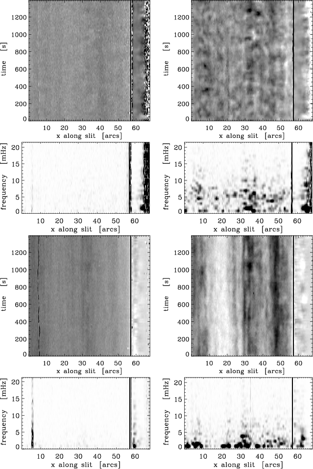 |
Figure 7:
Top panel: time variation of the line position
|
| Open with DEXTER | |
![\begin{figure}
\par\mbox{\includegraphics[width=6.7cm,clip]{h2929f16.ps} \hspace{1mm}
\includegraphics[width=6.7cm,clip]{h2929f17.ps} }
\end{figure}](/articles/aa/full/2001/44/aah2929/img40.gif) |
Figure 8:
Velocity (left) and intensity power (right) of He I 1083.0 nm along the slit in 2 frequency ranges (top: 4.2-6.4 mHz, bottom: 2.2-3.5 mHz), limb position is indicated at
|
| Open with DEXTER | |
![\begin{figure}
\par\mbox{\includegraphics[width=6.7cm,clip]{h2929f18.ps} \hspace{1mm}
\includegraphics[width=6.7cm,clip]{h2929f19.ps} }
\end{figure}](/articles/aa/full/2001/44/aah2929/img41.gif) |
Figure 9:
Example of a single line plot (top) and power spectrum (bottom) at
|
| Open with DEXTER | |
One of the central questions of this investigation concerns the height in the chromosphere where the two spectral lines originate. Figure 3 allows a direct comparison of them because
they were observed strictly simultaneously, with the same instrument and the reduction and analysis procedure were the same as well. The difference in height that we find is within the errors of
our measurement and analysis, which supports the idea that He D3 and He I 1083.0 nm come from the same height in the quiet solar atmosphere and react very similarly to the atmospheric conditions there
(changes in
![]() at
at
![]() of Fig. 4 are also very similar, we only have a constant offset in intensity between the two lines). We find considerable temporal as well as spatial variation of
of Fig. 4 are also very similar, we only have a constant offset in intensity between the two lines). We find considerable temporal as well as spatial variation of
![]() :
the time sequences of Fig. 3 range from rather constant values of 1600-1700 km (over 10 min) in #1, to a slow increase from 1200 to
1500 km in about half an hour in #2, and a sharp rise from 1500 to 1800 km within 1 min in #3. Including the results of data set #4 in Fig. 6, taken at the north pole of the sun, we get values as low as 1100 km and up to 1500 km over a range of
:
the time sequences of Fig. 3 range from rather constant values of 1600-1700 km (over 10 min) in #1, to a slow increase from 1200 to
1500 km in about half an hour in #2, and a sharp rise from 1500 to 1800 km within 1 min in #3. Including the results of data set #4 in Fig. 6, taken at the north pole of the sun, we get values as low as 1100 km and up to 1500 km over a range of
![]() .
Images of the Soft X-ray Telescope (SXT) of Yohkoh taken on the same day show that there was a large coronal hole at the north pole and we are sure that #4 was obtained inside this coronal hole.
.
Images of the Soft X-ray Telescope (SXT) of Yohkoh taken on the same day show that there was a large coronal hole at the north pole and we are sure that #4 was obtained inside this coronal hole.
The values in Fig. 6 are still well within the range of the other three data sets taken at the east and west limb.
In the following we compare our measurements with heights found in the literature: Table I of Penn & Jones (1996) summarizes D3 emission maxima obtained by various authors over the last 35 years and gives values between 1100 and 1800 km. Their own He I 1083.0 nm measurements (Table II) result in heights of about 2000 km and Schmidt et al. (1994) report 2200-2400 km.
These values are higher than ours but taking into account our own temporal and spatial variation of
![]() ,
we consider them within the possible range of values.
,
we consider them within the possible range of values.
Figures 7-9 summarize our analysis of the 23.5 min time sequence (#2). We measure line shifts due to the Doppler effect, thus we obtain the line-of-sight velocity of the plasma. As we approach the limb, the line-of-sight becomes more and more parallel to the solar surface and our off-limb emission measurements correspond to the horizontal component of the motion of the emitting plasma. Figures 7 (top half) and 8 (left) clearly show velocity oscillations in the 4-6 mHz regime both on disk and off-limb (see also Fig. 9). Since the He I lines are optically thin outside of prominences (Giovanelli & Hall 1977), one would expect any horizontal motion to cancel, but our spatial and temporal resolution is not sufficient to completely average out all horizontal velocities. The velocity signal is also the same in the two spectral lines, as can be seen in the example given in Fig. 9: the solid lines represent He I 1083.0 nm and the dashed ones He D3 in both the upper and lower part of the figure. Intensity oscillations (Fig. 7 (lower half) and Fig. 8 right) show very little power, except in the lowest frequencies. As our sequence is only 23.5 min long, we refrain from speculating about 10 or 15 min oscillations. The changes in intensity of the two spectral lines is the only other parameter that is not same, apart from the absolute intensity. Quiet sun chromospheric oscillations have been studied many times, mostly by means of photometry and spectroscopy in the Ca II H and K line, He I 1083.0 nm, the infrared CO lines (see reviews e.g. Rutten & Uitenbroek 1991; Rutten 1999). But all of them refer to disk center observations, thus, the suggested interpretations of the chromospheric oscillations consider the radial velocity field only (e.g. simulations of Carlsson & Stein 1995, which successfully reproduce internetwork CaIIK bright grains are purely one-dimensional).
Solanki et al. (1996) observed quiet sun chromospheric oscillations near the limb or off-limb in emission. They show power spectra of infrared CO lines very near the limb (
![]() 0.07-0.09). As the CO lines are formed in the cool part of the chromosphere, i.e. deeper than the He I lines it is not surprising that their power spectra (Fig. 2) look quite different from ours.
Penn & Allen (1997) calculate the center-to-limb variation of the velocity oscillation seen in He I 1083.0 nm and the photospheric Si I 1082.8 nm line. They find that the integrated power (in the p-mode frequency band of 2-6 mHz) decreases towards the limb in both lines and reaches about zero at the limb (determined from an extrapolation of the decrease of the integrated power) and they find no oscillation in their off-limb sequences. This does not agree with our results
(see Figs. 7-9). We think that this is probably due to their
strong spatial averaging (
0.07-0.09). As the CO lines are formed in the cool part of the chromosphere, i.e. deeper than the He I lines it is not surprising that their power spectra (Fig. 2) look quite different from ours.
Penn & Allen (1997) calculate the center-to-limb variation of the velocity oscillation seen in He I 1083.0 nm and the photospheric Si I 1082.8 nm line. They find that the integrated power (in the p-mode frequency band of 2-6 mHz) decreases towards the limb in both lines and reaches about zero at the limb (determined from an extrapolation of the decrease of the integrated power) and they find no oscillation in their off-limb sequences. This does not agree with our results
(see Figs. 7-9). We think that this is probably due to their
strong spatial averaging (
![]() on disk and 6
on disk and 6
![]() off-limb) possibly in addition to their limited spectral and temporal resolution (which they sacrificed to obtain a large spatial sampling). Nevertheless, a larger sample of high resolution time sequences is needed from the VTT (and from other observatories) to confirm our measurements .
off-limb) possibly in addition to their limited spectral and temporal resolution (which they sacrificed to obtain a large spatial sampling). Nevertheless, a larger sample of high resolution time sequences is needed from the VTT (and from other observatories) to confirm our measurements .
Several groups have studied spectral line shifts near the solar limb especially in coronal holes (although without temporal resolution). E.g. Dupree et al. (1996) look for the center to limb variation of the He I 1083.0 line in a more statistical way (using a few thousand line profiles). In coronal holes they find a systematic blue-ward line asymmetry in line profiles of the internetwork which they interpret as a radial outflow of the fast solar wind (this is in contradiction to measurements of Hassler et al. 1999, who find blueshifts of the coronal Ne VIII line in the network).
Peter (1999) observes blueshifts in the optically thick He I 58.4 nm line in coronal holes as well. But he does not interpret them as an outflow of the solar wind. Instead, he suggests that optical depth and radiative transfer effects are playing an important role in explaining his observations.
So what may be the nature of our observed horizontal oscillation? Kink modes of small scale magnetic elements would be a candidate. These kind of waves are of great interest in terms of chromospheric and coronal heating as they are easily excited due to their lower cut-off frequency, they do not suffer from radiative damping and do not produce shocks in higher layers of the atmosphere. Thus, they are capable of channeling energy from the convection zone into the corona. The excitation of these waves may either be due to collision of the fluxtubes with granules (Choudhuri et al. 1993) or by turbulence of the convection (Huang et al. 1995). Recently, kink waves of magnetic elements in the photosphere have been studied numerically by various groups (Ploner & Solanki 1997; Hasan & Kalkofen 1999; Hasan et al. 2000; Steiner et al. 1995, 1996), but hardly any direct observational evidence has been presented up to now (Ulrich 1996). Again, in a statistical sense we can interpret Stokes V zero-crossing rms velocities observed near the limb by Martínez Pillet et al. (1997) as transverse oscillations of photospheric fluxtubes, but without temporal resolution one can not exclude buffeting by granular convection as a source of their observed Doppler shifts.
Kalkofen (1997) suggests kink modes of small scale magnetic elements to explain the oscillations in chromospheric network bright points (observed at disk center). These kink modes would produce a signature of transverse waves at photospheric levels but due to mode coupling turn into longitudinal waves at the chromospheric level (and thus explain the heating in the network bright points). From our current observations we cannot tell, if they are taken in the network or the internetwork though the latter is more likely. Again, additional observations including imaging data may shed more light on this possibility.
Another explanation can be, that we see the extension of the global p-modes. Photospheric p-mode oscillations in the quiet sun are primarily vertical as shown by Stix & Wöhl (1974) and Schmidt et al. (1999). Nevertheless, p-modes with a large angular degree
![]() )
can reach the chromosphere due to a tunnel-effect (Dzhalilov et al. 2000, see their Fig. 2). As calculated in Dzhalilov et al. these p-modes have some of the properties we
observe here: (i) the relation of the horizontal to vertical velocity is large, so they are better seen near the limb, (ii) the modes are almost adiabatical, so they show very little intensity oscillation, (iii) the horizontal length-scale is a few 1000 km (as seen in Fig. 8, left), (iv)
3 min periods can more easily tunnel though the barrier.
)
can reach the chromosphere due to a tunnel-effect (Dzhalilov et al. 2000, see their Fig. 2). As calculated in Dzhalilov et al. these p-modes have some of the properties we
observe here: (i) the relation of the horizontal to vertical velocity is large, so they are better seen near the limb, (ii) the modes are almost adiabatical, so they show very little intensity oscillation, (iii) the horizontal length-scale is a few 1000 km (as seen in Fig. 8, left), (iv)
3 min periods can more easily tunnel though the barrier.
Acknowledgements
The VTT is operated on the island Tenerife by the Kiepenheuer Institut für Sonnenphysik in the Spanish Observatorio del Teide of the Instituto de Astrofisica de Canarias. We would like to thank Louise Harra-Murnion for providing the Yohkoh SXT images. Yohkoh is a mission of the Institute of Space and Astronautical Science of Japan. This research was partially supported by the European Commission through the TMR programme (European Solar Magnetometry Network). We would like to thank H. Balthasar, H. Peter and J. Staude for comments on the manuscript.