A&A 377, 589-608 (2001)
DOI: 10.1051/0004-6361:20011145
P. J. V. Garcia1,2,![]() - J. Ferreira3 - S. Cabrit4 -
L. Binette5
- J. Ferreira3 - S. Cabrit4 -
L. Binette5
1 - Centro de Astrofísica da Universidade do Porto,
Rua das Estrelas, 4150-762 Porto, Portugal
2 -
CRAL/Observatoire de Lyon, CNRS UMR 5574, 9 avenue
Charles André, 69561 St. Genis-Laval Cedex, France
3 -
Laboratoire d'Astrophysique de l'Observatoire de Grenoble,
BP 53, 38041 Grenoble Cedex, France
4 -
Observatoire de Paris,
DEMIRM, UMR 8540 du CNRS,
61 avenue de l'Observatoire,
75014 Paris, France
5 -
Instituto de Astronomía,
UNAM, Ap. 70-264, 04510 D. F., México
Received 21 March 2001 / Accepted 3 August 2001
Abstract
Motivated by recent subarcsecond resolution observations of jets
from T Tauri stars, we extend the work of Safier (1993a,b) by computing the thermal and ionization structure of
self-similar, magnetically-driven, atomic disk winds heated by
ambipolar diffusion. Improvements over his work include: (1) new
magnetized cold jet solutions consistent with the underlying
accretion disk (Ferreira 1997); (2) a more accurate treatment
of ionization and ion-neutral momentum exchange rates; and (3)
predictions for spatially resolved forbidden line emission (maps,
long-slit spectra, and line ratios), presented in a companion
paper, Garcia et al. (2001b). As in Safier (1993a), we obtain jets with a temperature
plateau around 104 K, but ionization fractions are revised
downward by a factor of 10-100. This is due to previous omission
of thermal speeds in ion-neutral momentum-exchange rates and to
different jet solutions. The physical origin of the hot
temperature plateau is outlined. In particular we present three
analytical criteria for the presence of a hot plateau, applicable
to any given MHD wind solution where ambipolar diffusion and
adiabatic expansion are the dominant heating and cooling terms.
We finally show that, for solutions favored by observations, the
jet thermal structure remains consistent with the usual
approximations used for MHD jet calculations (thermalized,
perfectly conducting, single hydromagnetic cold fluid
calculations).
Key words: ISM: jets and outflows - stars: pre-main sequence - MHD - line: profiles - accretion disks
Progresses in long slit differential astrometry techniques and high angular resolution imaging from Adaptive Optics and the Hubble Space Telescope have shown that the high velocity forbidden emission observed in Classical T Tauri Stars (CTTSs) is related to collimated (micro-)jets (e.g. Solf 1989; Solf & Böhm 1993; Ray et al. 1996; Hirth et al. 1997; Lavalley-Fouquet et al. 2000; Dougados et al. 2000; Bacciotti et al. 2000). Although outflow activity is known to decrease with age (Bontemps et al. 1996), CTTSs still harbor considerable activity (e.g. Mundt & Eislöffel 1998) and present the advantage of not being embedded. It is now commonly believed that such jets are magnetically self-confined, by a "hoop stress'' due to a non-vanishing poloidal current (Chan & Henriksen 1980; Heyvaerts & Norman 1989). The main reason lies in the need to produce highly supersonic unidirectional flows. Indeed, this requires an acceleration process that is closely related to the confining mechanism. The most promising models of jet production rely therefore on the presence of large scale magnetic fields, extracting energy and mass from a rotating object. However, we still do not know precisely what the jet driving sources are. Moreover, observed jets harbor time-dependent features, with time-scales ranging from tens to thousands of years. Such time-scales are much longer than those involving the protostar or the inner accretion disk. Therefore, although the possibility remains that jets have a non-stationary origin (e.g. Ouyed & Pudritz 1997; Goodson et al. 1999), only steady-state models will be addressed here.
Stationary stellar wind models have been developed (e.g. Sauty & Tsinganos 1994), however observed correlations between signatures of accretion and ejection clearly show that the disk is an essential ingredient in jet formation (Cohen et al. 1989; Cabrit et al. 1990; Hartigan et al. 1995). Therefore we expect accretion and ejection to be interdependent, through the action of magnetic fields. There are mainly two classes of stationary magnetized disk wind models, depending on the radial extent of the wind-producing region in the disk. In the first class (usually referred to as "disk winds''), a large scale magnetic field threads the disk on a large region (Blandford & Payne 1982; Wardle & Koenigl 1993; Ferreira & Pelletier 1993,1995; Li 1995; Li 1996; Ferreira 1997; Krasnopolsky et al. 1999; Casse & Ferreira 2000a,b; Vlahakis et al. 2000). Such a field is assumed to arise from both advection of interstellar magnetic field and local dynamo generation (Rekowski et al. 2000). In the second class of models (referred to as "X-winds''), only a tiny region around the disk inner edge produces a jet (Camenzind 1990; Shu et al. 1994; Shu et al. 1995; Shu et al. 1996; Lovelace et al. 1999). The magnetic field is assumed to originally come from the protostar itself, after some eruptive phase that linked the disk inner edge to the protostellar magnetosphere. Note that in both models, jets extract angular momentum and mass from the underlying portion of the disk. However, by construction, "disk-winds'' are produced from a large spread in radii, while "X-winds'' arise from a single annulus. Apart from distinct disk physics, the difference in size and geometry of the ejection regions should also introduce some observable jet features. Another scenario has been proposed, where the protostar produces a fast collimated jet surrounded by a slow uncollimated disk wind or disk corona (Kwan & Tademaru 1988,1995; Kwan 1997), but such a scenario still lacks detailed calculations.
So far, all disc-driven jet calculations used a "cold'' approximation, i.e. negligible thermal pressure gradients. Therefore, each magnetic surface is assumed either isothermal or adiabatic. But to test which class of models is at work in T Tauri stars, reliable observational predictions must be made and the thermal equilibrium needs then to be solved along the flow. Such a difficult task is still not addressed in a fully self-consistent way, namely by solving together the coupled dynamics and energy equations. Thus, no model has been able yet to predict the gas excitation needed to generate observational predictions.
One first possibility is to use a posteriori a simple parameterization for the temperature and ionization fraction evolution along the flow. This was done by Shang et al. (1998) and Cabrit et al. (1999) for X-winds and disk winds respectively. These approaches are able to predict the rough jet morphology, but do not provide reliable flux and line profile predictions, since the thermal structure lacks full physical consistency.
The second possibility is to solve the thermal evolution a posteriori, with the difficulty of identifying the heating sources (subject to the constraint of consistency with the underlying dynamical solution). Several heating sources are indeed possible: (1) planar shocks (e.g. Hartigan et al. 1987,1994); (2) oblique magnetic shocks in recollimating winds (Ouyed & Pudritz 1993,1994); (3) turbulent mixing layers (e.g. Binette et al. 1999); and (4) current dissipation by ion-neutral collisions, referred to as ambipolar diffusion heating (Safier 1993a,1993b). A further heating scenario (not yet explored in the context of MHD jets and only valid in some environments) is photoionization from OB stars (Reipurth et al. 1998; Raga et al. 2000; Bally & Reipurth 2001). Of all these previous mechanisms only ambipolar diffusion heating allows "minimal'' thermal solutions, in the sense that the same physical process - non-vanishing currents - is responsible for jet dynamics and heating. As a consequence no additional tunable parameter is invoked for the thermal description. Furthermore, Safier (1993b) was able to obtain fluxes and profiles in reasonable agreement with observations. In this paper, we extend the work of Safier (1993a,1993b) by (1) using magnetically-driven jet solutions self-consistently computed with the underlying accretion disk, and (2) a more accurate treatment of ionization using the Mappings Ic code and ion-neutral momentum exchange rates which include the thermal contribution. In a companion paper (Garcia et al. 2001, hereafter Paper II), we generate predictions for spatially resolved orbidden line emission maps, long-slit spectra, and line ratios.
This article is structured as follows: in Sect. 2 we introduce the dynamical structure of the disk wind under study, and present physical values of the density, velocity, magnetic field, and Lorentz force along streamlines; in Sect. 3 we describe the physical processes taken into account in the thermal evolution computations, whose results are presented and discussed in Sect. 4. Conclusions are presented in Sect. 5. Some important derivations, dust description and consistency checks of our calculations are presented in the appendices.
A precise disk wind theory must explain how much matter is deviated from radial to vertical motion, as well as the amount of energy and angular momentum carried away. This implies a thorough treatment of both the disk interior and its matching with the jets, namely to consider magnetized accretion-ejection structures (hereafter MAES). The only way to solve such an entangled problem is to take into account all dynamical terms, a task that can be properly done within a self-similar framework.
In this paper, we use the models of Ferreira (1997) describing
steady-state, axisymmetric MAES under the following assumptions: (i) a
large scale magnetic field of bipolar topology is threading a
geometrically thin disk; (ii) its ionization is such that MHD applies
(neutrals are well-coupled to the magnetic field); (iii) some active
turbulence inside the disk produces anomalous diffusion allowing
matter to cross the field lines. Two extra simplifying assumptions
were used: (iv) jets are assumed to be cold, i.e. powered by the
magnetic Lorentz force only (the centrifugal force is due to the
Lorentz azimuthal torque), with isothermal magnetic surfaces (the
midplane temperature varying as
![]() )
and (v) jets
carry away all disk angular momentum. This last assumption has been
removed only recently by Casse & Ferreira (2000a).
)
and (v) jets
carry away all disk angular momentum. This last assumption has been
removed only recently by Casse & Ferreira (2000a).
All solutions obtained so far display the same asymptotic behavior. After an opening of the jet radius leading to a very efficient acceleration of the plasma, the jet undergoes a refocusing towards the axis (recollimation). All self-similar solutions are then terminated, most probably producing a shock (Gomez de Castro & Pudritz 1993; Ouyed & Pudritz 1993). This systematic behavior could well be imposed by the self-similar geometry itself and not be a general result (Ferreira 1997). Nevertheless, such a shock would occur in the asymptotic region, far away from the disk. Thus, we can confidently use these solutions in the acceleration zone, where forbidden emission lines are believed to be produced (Hartigan et al. 1995).
The isothermal self-similar MAES considered here are described with
three free dimensionless local parameters (see Ferreira 1997, for more
details) and four global quantities:
(1) the disk aspect ratio
 |
(1) |
| (2) |
 |
(3) |
For our present study, we keep only ![]() and
and
![]() as
free parameters and fix the values of the other five as follows: The
disk aspect ratio was measured by Burrows et al. (1996) for HH 30 as
as
free parameters and fix the values of the other five as follows: The
disk aspect ratio was measured by Burrows et al. (1996) for HH 30 as ![]() 0.1
so we fix
0.1
so we fix
![]() .
The MHD turbulence parameter is
taken
.
The MHD turbulence parameter is
taken
![]() in order to have powerful jets
(Ferreira 1997). The stellar mass is fixed at
in order to have powerful jets
(Ferreira 1997). The stellar mass is fixed at
![]() ,
typical for T Tauri stars, and the inner radius of the MAES
is set to
,
typical for T Tauri stars, and the inner radius of the MAES
is set to
![]() 0.07 AU (typical disk corotation radius
for a 10 days rotation period): inside this region the magnetic field
topology could be significantly affected by the stellar
magnetosphere-disk interaction. The outer radius is kept at
0.07 AU (typical disk corotation radius
for a 10 days rotation period): inside this region the magnetic field
topology could be significantly affected by the stellar
magnetosphere-disk interaction. The outer radius is kept at
![]() for consistency with the one fluid
approximation (Appendix C) and the atomic gas description.
Regarding atomic consistency, Safier (1993a) solved the flow
evolution assuming inicially all H bound in H2. He found H2 to
completely dissociate at the wind base, for small
for consistency with the one fluid
approximation (Appendix C) and the atomic gas description.
Regarding atomic consistency, Safier (1993a) solved the flow
evolution assuming inicially all H bound in H2. He found H2 to
completely dissociate at the wind base, for small ![]() .
However, after a critical flow line footpoint H2 would not
completely dissociate, therefore affecting the thermal solution. This
critical footpoint was at 3 AU for his MHD solution nearer our
parameter space.
.
However, after a critical flow line footpoint H2 would not
completely dissociate, therefore affecting the thermal solution. This
critical footpoint was at 3 AU for his MHD solution nearer our
parameter space.
We note that our two free parameters are still bounded by
observational constraints: mass conservation relates the ejection
index ![]() to the accretion/ejection rates ratios,
to the accretion/ejection rates ratios,
| (4) |
Table 1 provides a list of some disk and jet parameters.
These local parameters were constrained by steady-state requirements,
namely the smooth crossing of MHD critical points. Disk parameters are
useful to give us a view of the physical conditions inside the disk.
Thus, the required magnetic field B0 at the disk midplane and at a
radial distance ![]() is
is
| (6) |
 |
= |  |
|
| (7) |
| Solution |
|
|
||||
| A | 0.010 | 0.729 | 1.46 | 0.014 | 41.6 | 50.6 |
| B | 0.007 | 0.690 | 1.46 | 0.011 | 59.4 | 52.4 |
| C | 0.005 | 0.627 | 1.52 | 0.009 | 84.2 | 55.4 |
![\begin{figure}
\par\includegraphics[width=6.8cm,clip]{fig1_new.epsi} %
\end{figure}](/articles/aa/full/2001/38/aa1260/img103.gif) |
Figure 1:
Several wind quantities along a streamline for
model A (long-dashed line), B (solid) and C (dashed): jet nuclei
density |
| Open with DEXTER | |
In order to obtain a solution for the MAES, a variable separation
method has been used allowing to transform the set of coupled
partially differential equations into a set of coupled ordinary
differential equations (ODEs). Hence, the solution in the
![]() space is obtained by solving for a flow line and then scaling this
solution to all space. Once a solution is found (for a given set of
parameters in Sect. 2.2), the evolution of all wind
quantities Q along any flow line is given by:
space is obtained by solving for a flow line and then scaling this
solution to all space. Once a solution is found (for a given set of
parameters in Sect. 2.2), the evolution of all wind
quantities Q along any flow line is given by:
| (8) |
Under stationarity, the thermal structure of an atomic (perfect) gas
with density n and temperature T is given by the first law of
thermodynamics:
The gas considered here is composed of electrons, ions and neutrals of
several atomic species, namely
![]() where the overline stands for a sum over all present
chemical elements. We then define the density of nuclei
where the overline stands for a sum over all present
chemical elements. We then define the density of nuclei
![]() and the electron density
and the electron density
![]() .
Correspondingly, the total velocity
.
Correspondingly, the total velocity ![]() appearing in Eq. (10) must be understood as the
barycentric velocity. As usual in one-fluid approximation, we suppose
- and verify it in Sect. C.1 - all species well
coupled (through collisions), so that they share the same temperature
T. We also assume that no molecule formation occurs, so that mass
conservation requires
appearing in Eq. (10) must be understood as the
barycentric velocity. As usual in one-fluid approximation, we suppose
- and verify it in Sect. C.1 - all species well
coupled (through collisions), so that they share the same temperature
T. We also assume that no molecule formation occurs, so that mass
conservation requires
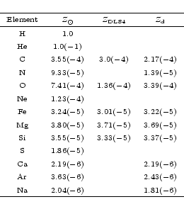
We solve the gas ionization state (Eqs. (12) to (14)) using the Mappings Ic code - Binette et al. (1985); Binette & Robinson (1987); Ferruit et al. (1997). This code considers atomic gas composed by the chemical elements H, He, C, N, O, Ne, Fe, Mg, Si, S, Ca, Ar. We also added Na (whose ionization evolution is not solved by Mappings Ic), assuming it to be completely ionized in Na II. Hydrogen and Helium are treated as five level atoms.
The rate equations solved by Mappings Ic include photoionization, collisional ionization, secondary ionization due to energetic photoelectrons, charge exchange, recombination and dielectronic recombination. This is in contrast with Safier, who assumed a fixed ionization fraction for the heavy elements and solved only for the ionization evolution of H and He, considering two levels for H and only the ground level for He.
The adopted abundances are presented in Table 2. In contrast with Safier, we take into account heavy element depletion onto dust grains (see Sect. 3.2.3 and Appendix B) in the dusty region of the wind.
|
For simplicity, the central source radiation field is described in exactly the same way as in Safier and we refer the reader to the expressions (C1-C10) presented in his Appendix C. This radiation field is diluted with distance but is also absorbed by intervening wind material ejected at smaller radii.
We treat the radiative transfer as a simple absorption of the diluted
central source, namely
We now address the question of optical depth. In our model, the flow
is hollow, starting from a ring located at the inner disk radius
![]() and extending to the outer radius
and extending to the outer radius
![]() .
The jet inner boundary is therefore exposed to the central ionizing
radiation, which produces then a small layer where hydrogen is
completely photoionized. The width
.
The jet inner boundary is therefore exposed to the central ionizing
radiation, which produces then a small layer where hydrogen is
completely photoionized. The width ![]() of this layer can be
computed by equating the number of emitted H ionizing photons,
of this layer can be
computed by equating the number of emitted H ionizing photons,
![]() ,
to the
number of recombinations in this layer,
,
to the
number of recombinations in this layer,
![]() for our geometry. We found that
for our geometry. We found that
![]() ,
and thus assume that all photons capable of ionizing hydrogen are
exhausted within this thin shell. Furthermore, there is presumably
matter in the inner "hollow'' region, so the previous considerations
are upper limits.
,
and thus assume that all photons capable of ionizing hydrogen are
exhausted within this thin shell. Furthermore, there is presumably
matter in the inner "hollow'' region, so the previous considerations
are upper limits.
For the heavy elements, photoionization optical depths are negligible,
due to the much smaller abundances, and are thus ignored. The opacity
![]() is assumed to be dominated by dust absorption (see
Appendix B for details). Dust will influence the
ionization structure at the base of the flow, where ionization is
dominated by heavy elements.
is assumed to be dominated by dust absorption (see
Appendix B for details). Dust will influence the
ionization structure at the base of the flow, where ionization is
dominated by heavy elements.
To summarize, the adopted radiation field is a central source absorbed by dust, with a cutoff at and above the Hydrogen ionization frequency.
Safier showed that if dust exists inside the disk, then the wind drag will lift the dust thereby creating a dusty wind. Our wind shares the same property. We model the dust (Appendix B) as a mix of graphite and astronomical silicate, with a MRN size distribution and use for the dust optical properties the tabulated values of Draine & Lee (1984), Draine & Malhotra (1993), Laor & Draine (1993). For simplicity we assumed the dust to be stationary, in thermodynamic equilibrium with the central radiation field and averaged all dust quantities by the MRN size distribution.
In addition, we take into account depletion of heavy elements into the
dust phase. This effect was not considered by Safier.
In Table 2 we present the dust phase abundances needed to maintain the
MRN distribution (Draine & Lee), and our adopted depleted
abundances, taken from observations of diffuse clouds toward ![]() Ori (Savage & Sembach 1996). These are more realistic, although presenting
less depletion of carbon than required by MRN. Depletion has only a
small effect on the calculated wind thermal structure, but can be
significant when comparing to observed line ratios based on depleted
elements.
Ori (Savage & Sembach 1996). These are more realistic, although presenting
less depletion of carbon than required by MRN. Depletion has only a
small effect on the calculated wind thermal structure, but can be
significant when comparing to observed line ratios based on depleted
elements.
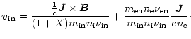
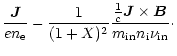
The dissipation of electric currents ![]() provides a local heating
term per unit volume
provides a local heating
term per unit volume
![]() ,
where
,
where ![]() and
and ![]() are the
electric and magnetic fields,
are the
electric and magnetic fields, ![]() the fluid velocity and cthe speed of light. In a multi-component gas, with electrons and
several ion and neutral species, the generalized Ohm's law writes
the fluid velocity and cthe speed of light. In a multi-component gas, with electrons and
several ion and neutral species, the generalized Ohm's law writes
 |
(16) |
The first term appearing in the right hand side of the generalized
Ohm's law is the usual Ohm's term, while the second describes the
ambipolar diffusion, the third is the electric field due to the
electron pressure and the last is the Hall term. This last effect
provides no net dissipation in contrary to the other three. It turns
out that the dissipation due to the electronic pressure is quite
negligible and has been therefore omitted (Appendix C).
Thus, the MHD dissipation writes
An important difference with Safier is that we take
into account thermal speeds in ion-neutral momentum exchange rate
coefficients. This increases
![]() ,
and results in significantly
smaller ionization fractions (Sect. 4.8).
,
and results in significantly
smaller ionization fractions (Sect. 4.8).
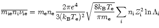
Both collisional ionization cooling
![]() and
radiative recombination cooling
and
radiative recombination cooling
![]() effects are
taken into account by Mappings Ic. These terms are given by,
effects are
taken into account by Mappings Ic. These terms are given by,
| = |  |
(18) | |
| = |  |
(19) |
These ionization/recombination effects, taken into account in part by Safier, are in general smaller than adiabatic and line cooling.
Photoionization by the radiation field, not taken into account by
Safier, provides an extra source of heating
![]() .
This term, which is also computed by Mappings Ic, is given by
.
This term, which is also computed by Mappings Ic, is given by
 |
(20) |
Collisionally excited lines provide a very efficient way to cool the
gas, thanks to an extensive set of resonance and inter-combination
lines, as well as forbidden lines. This radiative cooling
![]() is computed by Mappings Ic by solving for
each atom the local statistical equilibrium, and will allow us to
compute emission maps and line profiles for comparison with
observations (see Garcia et al. 2001). We include cooling by
hydrogen lines,
is computed by Mappings Ic by solving for
each atom the local statistical equilibrium, and will allow us to
compute emission maps and line profiles for comparison with
observations (see Garcia et al. 2001). We include cooling by
hydrogen lines,
![]() ,
in particular H
,
in particular H![]() ,
which could not be computed by Safier (two-level atom
description).
,
which could not be computed by Safier (two-level atom
description).
Several processes, also computed by Mappings Ic, appeared to be very small and not affecting the jet thermal structure. We just cite them here for completeness: free-free cooling and heating, two-photon continuum and Compton scattering.
We ignored thermal conduction, which could be relevant along flow lines, the magnetic field reducing the gas thermal conductibility in any other direction. Also ignored was gas cooling by dust grains and heating by cosmic rays. We checked a posteriori that these three terms indeed have a negligible contribution (see Appendix C.2).
In our study, flow thermodynamics are decoupled from the dynamics -
cold jet approximation. The previous Eqs. (10) to (14) can then be integrated for a given flow pattern.
The dynamical quantities (density, velocity and magnetic fields) are
given by the cold MHD solutions presented in Sect. 2. For
the steady-state, axisymmetric, self-similar MHD winds under study,
any total derivative writes
 |
(21) |
The integration of the set Eqs. (12) to (14) and (22) along the flow is an initial value problem. Thus, some way to estimate the initial temperature and populations must be devised. All calculations start at the slow-magnetosonic (SM) point, which is roughly at two scale heights above the disk midplane (for the solutions used here).
To estimate the initial temperature, Safier equated
the poloidal flow speed at the SM point to the sound speed. Although
this estimation agrees with cold flow theory, it is inconsistent with
the energy equation which is used further up in the jet. Our approach
was then to compute the initial temperature and ionic populations
assuming that
 |
(23) |
The initial populations are computed by Mappings Ic assuming ionization equilibrium with the incoming radiation field. However for high accretion rates and for the outer zones of the wind, dust opacity and inclination effects shield completely the ionizing radiation field. The temperature is too low for collisional ionization to be effective. The ionization fraction thus reaches our prescribed minimum - all Na is in the form Na II (Table 2) and all the other elements (computed by Mappings Ic) neutral. However, soon the gas flow gains height and the ionization field is strong enough such that the ionization is self-consistently computed by Mappings Ic.
After obtaining an initial temperature and ionization state for the
gas we proceed by integrating the system of equations. In practice the
ionization evolution is computed by Mappings Ic and separately
we integrate Eq. (22) with a Runge-Kutta type algorithm
(Press et al. 1988). We maintain both the populations and Mappings Ic cooling/heating rates per
![]() fixed during each
temperature integrating spatial step. After we call Mappings Ic
to evolve the populations and rates, at the new temperature, during
the time taken by the fluid to move the spatial step. This step is
such, that the RK integration has a numerical accuracy of 10-6and, that the newly computed temperature varies by less than a factor
of 10-4. Such a small variation in temperature allows us to
assume constant rates and populations while solving the energy
equation. We checked a few integrations by redoing them at half the
step used and found that the error in the ionic fraction is
<10-3in the jet, and
< 10-2 in the recollimation zone; the temperature
precision being roughly a few times better. This ensures an intrinsic
numerical precision comfortably below the accuracy of the atomic data
and the
fixed during each
temperature integrating spatial step. After we call Mappings Ic
to evolve the populations and rates, at the new temperature, during
the time taken by the fluid to move the spatial step. This step is
such, that the RK integration has a numerical accuracy of 10-6and, that the newly computed temperature varies by less than a factor
of 10-4. Such a small variation in temperature allows us to
assume constant rates and populations while solving the energy
equation. We checked a few integrations by redoing them at half the
step used and found that the error in the ionic fraction is
<10-3in the jet, and
< 10-2 in the recollimation zone; the temperature
precision being roughly a few times better. This ensures an intrinsic
numerical precision comfortably below the accuracy of the atomic data
and the
![]() collision cross-sections
which, coupled to abundance incertitudes, are the main limitating
factors. Details on the actual numerical procedure used by Mappings Ic to compute the non-equilibrium gas evolution are given in
Binette et al. (1985).
collision cross-sections
which, coupled to abundance incertitudes, are the main limitating
factors. Details on the actual numerical procedure used by Mappings Ic to compute the non-equilibrium gas evolution are given in
Binette et al. (1985).
In this section we present the calculated thermal and ionization
structure along wind flow lines, discuss the physical origin of the
temperature plateau and its connection with the underlying MHD
solution, discuss the effect of various key model parameters and
finally compare our results with those found by
Safier. The parameters spanned for the calculation of
the thermal solutions are the wind ejection index ![]() describing the
flow line geometry, the mass accretion rate
describing the
flow line geometry, the mass accretion rate
![]() and
the cylindrical radius
and
the cylindrical radius ![]() where the field is anchored in the
disk.
where the field is anchored in the
disk.
In Fig. 2, solid curves present the out of ionization
equilibrium evolution of temperature, electronic density, and proton
fraction along flow lines with
![]() and 1 AU, as a
function of
and 1 AU, as a
function of
![]() ,
for accretion rates ranging from
10-8 to
,
for accretion rates ranging from
10-8 to
![]() yr-1. For comparison
purposes, dashed curves plot the same quantities calculated assuming
ionization equilibrium at the local temperature and radiation field.
For compactness we present only these detailed results for our model
B, with an intermediate ejection index
yr-1. For comparison
purposes, dashed curves plot the same quantities calculated assuming
ionization equilibrium at the local temperature and radiation field.
For compactness we present only these detailed results for our model
B, with an intermediate ejection index
![]() .
We divide the
flow in three regions: the base, the jet and the recollimation zone.
These regions are separated by the Alfvén point and the
recollimation point (where the axial distance reaches its maximum).
We only present the initial part of the recollimation zone here,
because the dynamical solution is less reliable further out, where gas
pressure is increased by compression and may not be negligible
anymore. Note that the recollimation zone was not yet reached over
the scales of interest in the solutions used by
Safier.
.
We divide the
flow in three regions: the base, the jet and the recollimation zone.
These regions are separated by the Alfvén point and the
recollimation point (where the axial distance reaches its maximum).
We only present the initial part of the recollimation zone here,
because the dynamical solution is less reliable further out, where gas
pressure is increased by compression and may not be negligible
anymore. Note that the recollimation zone was not yet reached over
the scales of interest in the solutions used by
Safier.
![\begin{figure}
\par\includegraphics[width=6.5cm,clip]{fig2.epsi} %
\end{figure}](/articles/aa/full/2001/38/aa1260/img190.gif) |
Figure 2:
Several wind quantities versus
|
| Open with DEXTER | |
The gas temperature increases steeply at the wind base (after an
initial cooling phase for high
![]() yr-1). It then stabilizes in a hot temperature
plateau around
yr-1). It then stabilizes in a hot temperature
plateau around ![]() 1-3
1-3
![]() K, before increasing again
after the recollimation point through compressive heating. The plateau
is reached further out for larger accretion rates and larger
K, before increasing again
after the recollimation point through compressive heating. The plateau
is reached further out for larger accretion rates and larger
![]() .
Its temperature decreases with increasing
.
Its temperature decreases with increasing
![]() .
The temperature plateau and its behavior with
.
The temperature plateau and its behavior with
![]() were first identified by Safier in his wind
solutions. We will discuss in Sect. 4.4 why they
represent a robust property of magnetically-driven disk winds heated
by ambipolar diffusion.
were first identified by Safier in his wind
solutions. We will discuss in Sect. 4.4 why they
represent a robust property of magnetically-driven disk winds heated
by ambipolar diffusion.
The bottom panels of Fig. 2 plot the proton fraction
![]() along the flow lines. It rises
steeply with wind temperature through collisional ionization, reaching
a value
along the flow lines. It rises
steeply with wind temperature through collisional ionization, reaching
a value
![]() at the beginning of the temperature plateau.
Beyond this point, it continues to increase but starts to "lag
behind'' the ionization equilibrium calculations (dashed curves): the
density decline in the expanding wind increases the ionization and
recombination timescales. Eventually, for
at the beginning of the temperature plateau.
Beyond this point, it continues to increase but starts to "lag
behind'' the ionization equilibrium calculations (dashed curves): the
density decline in the expanding wind increases the ionization and
recombination timescales. Eventually, for
![]() ,
density
is so low that these timescales become longer than the dynamical ones,
and the proton fraction becomes completely "frozen-in'' at a constant
level, typically a factor 2-3 below the value found in ionization
equilibrium calculations (dashed curves).
,
density
is so low that these timescales become longer than the dynamical ones,
and the proton fraction becomes completely "frozen-in'' at a constant
level, typically a factor 2-3 below the value found in ionization
equilibrium calculations (dashed curves).
The electron density (![]() )
evolution is shown in the middle
panels of Fig. 2. In the jet region, where
)
evolution is shown in the middle
panels of Fig. 2. In the jet region, where ![]() is roughly constant, the dominant decreasing pattern with
is roughly constant, the dominant decreasing pattern with ![]() is
set by the wind density evolution as the gas speeds up and
expands. Similarly, the rise in
is
set by the wind density evolution as the gas speeds up and
expands. Similarly, the rise in ![]() in the recollimation zone
is due to gas compression. A remarkable result is that, as long as
ionization is dominated by hydrogen (i.e.
in the recollimation zone
is due to gas compression. A remarkable result is that, as long as
ionization is dominated by hydrogen (i.e.
![]() ),
), ![]() is not highly dependent of
is not highly dependent of
![]() ,
increasing by a factor of 10 only over three orders in magnitude in
accretion rate. This indicates a roughly inverse scaling of
,
increasing by a factor of 10 only over three orders in magnitude in
accretion rate. This indicates a roughly inverse scaling of ![]() with
with
![]() (bottom panels of Fig. 2),
a property already found by Safier which we will
discuss in more detail later.
(bottom panels of Fig. 2),
a property already found by Safier which we will
discuss in more detail later.
In regions at the wind base where
![]() ,
variations
of
,
variations
of ![]() are linked to the detailed photoionization of heavy
elements which are then the dominant electron donors. The respective
contributions of various ionized heavy atoms to the electronic
fraction
are linked to the detailed photoionization of heavy
elements which are then the dominant electron donors. The respective
contributions of various ionized heavy atoms to the electronic
fraction ![]() is illustrated in Fig. 3 for
is illustrated in Fig. 3 for
![]() yr-1. While
O II and N II are strongly coupled to hydrogen
collisional ionization through charge exchange reactions, the other
elements are dominated by photoionization. The sharp discontinuity in
C II and Na II at the wind base for
yr-1. While
O II and N II are strongly coupled to hydrogen
collisional ionization through charge exchange reactions, the other
elements are dominated by photoionization. The sharp discontinuity in
C II and Na II at the wind base for
![]() AU
is caused by the crossing of the dust sublimation surface by the
streamline (see Appendix B). Inside the surface we are in
the dust sublimation zone where heavy atoms are consequently not
depleted onto grains and hence have a higher abundance. In contrast,
for
AU
is caused by the crossing of the dust sublimation surface by the
streamline (see Appendix B). Inside the surface we are in
the dust sublimation zone where heavy atoms are consequently not
depleted onto grains and hence have a higher abundance. In contrast,
for
![]() AU, the flow starts already outside the
sublimation radius, in a region well-shielded from the UV flux of the
boundary-layer, where only Na is ionized. Extinction progressively
decreases as material is lifted above the disk plane and sulfur, then
carbon, also become completely photoionized.
AU, the flow starts already outside the
sublimation radius, in a region well-shielded from the UV flux of the
boundary-layer, where only Na is ionized. Extinction progressively
decreases as material is lifted above the disk plane and sulfur, then
carbon, also become completely photoionized.
![\begin{figure}
\par\includegraphics[width=8.5cm,clip]{fig3.epsi} %
\end{figure}](/articles/aa/full/2001/38/aa1260/img200.gif) |
Figure 3:
Ion abundances with respect to hydrogen
(
|
| Open with DEXTER | |
The heating and cooling terms along the streamlines for our out of
equilibrium calculations are plotted in Fig. 4 for
![]() and 1 AU, and for two values of
and 1 AU, and for two values of
![]() = 10-6 and
= 10-6 and
![]() yr-1.
yr-1.
![\begin{figure}
\par\includegraphics[width=9cm,clip]{fig4.epsi}\end{figure}](/articles/aa/full/2001/38/aa1260/img203.gif) |
Figure 4:
Heating and cooling processes (in erg s-1 cm-3)
along the flow line versus
|
| Open with DEXTER | |
Before the recollimation point, the main cooling process throughout
the flow is adiabatic cooling
![]() ,
although Hydrogen
line cooling
,
although Hydrogen
line cooling
![]() is definitely not
negligible. The main heating process is ambipolar diffusion
is definitely not
negligible. The main heating process is ambipolar diffusion
![]() .
The only exception occurs at the wind base for
small
.
The only exception occurs at the wind base for
small
![]() 0.1 AU and large
0.1 AU and large
![]() yr-1, where photoionization heating
yr-1, where photoionization heating
![]() initially dominates. Under such conditions,
ambipolar diffusion heating is low due to the high ion density, which
couples them to neutrals and reduces the drift responsible for drag
heating. However,
initially dominates. Under such conditions,
ambipolar diffusion heating is low due to the high ion density, which
couples them to neutrals and reduces the drift responsible for drag
heating. However,
![]() decays very fast due to the
combined effects of radiation dilution, dust opacity, depletion of
heavy atoms in the dust phase, and the decrease in gas density. At the
same time, the latter two effects make
decays very fast due to the
combined effects of radiation dilution, dust opacity, depletion of
heavy atoms in the dust phase, and the decrease in gas density. At the
same time, the latter two effects make
![]() rise and
become quickly the dominant heating term. In the recollimation zone,
the main cooling process is hydrogen line cooling
rise and
become quickly the dominant heating term. In the recollimation zone,
the main cooling process is hydrogen line cooling
![]() ,
and the main heating term is compression heating
(
,
and the main heating term is compression heating
(
![]() is negative).
is negative).
A striking result in Fig. 4, also found by
Safier, is that a close match is quickly established
along each streamline between
![]() and
and
![]() ,
and is maintained until the recollimation region. The value of
,
and is maintained until the recollimation region. The value of
![]() where this balance is established is also where the temperature
plateau starts. We will demonstrate below why this is so for the
class of MHD wind solutions considered here.
where this balance is established is also where the temperature
plateau starts. We will demonstrate below why this is so for the
class of MHD wind solutions considered here.
The existence of a hot temperature plateau where
![]() exactly balances
exactly balances
![]() is the most remarkable and robust
property of magnetically-driven disk winds heated by ambipolar
diffusion. Furthermore, it occurs throughout several decades along
the flow including the zone of the jet that current observations are
able to spatially resolve.
is the most remarkable and robust
property of magnetically-driven disk winds heated by ambipolar
diffusion. Furthermore, it occurs throughout several decades along
the flow including the zone of the jet that current observations are
able to spatially resolve.
In this section, we explore in detail which generic properties of our
MHD solution allow a temperature plateau at
![]() K to be
reached, and why this equilibrium may not be reached for other MHD
wind solutions.
K to be
reached, and why this equilibrium may not be reached for other MHD
wind solutions.
First, we note that the energy equation (Eq. (22)) in the
region where drag heating and adiabatic cooling are the dominant terms
(which includes the plateau region) can be cast in the simplified
form:
| (27) |
| |
Figure 5:
Left: function F(T) in erg g cm3 s-1versus temperature assuming local ionization equilibrium and an
ionization flux that ionizes only all Na and all C. Center:
function |
| Open with DEXTER | |
The "wind function'' G is plotted in the center panel of
Fig. 5 for our 3 solutions. It rises by 5 orders of
magnitude at the wind base and then stabilizes in the jet region
(until it diverges to infinity near the recollimation point). The
physical reason for its behavior is better seen if we note that the
main force driving the flow is the Lorentz force:
| (28) |
The "ionization function'' F is in general a rising function of Tand is plotted in the left panel of Fig. 5 under the
approximation of local ionization equilibrium. Two regimes are
present: in the low temperature regime, ![]()
![]() is
dominated by the abundance of photoionized heavy elements and
is
dominated by the abundance of photoionized heavy elements and
![]() increases linearly with T, for fixed
increases linearly with T, for fixed ![]() .
The effect of the UV flux in this region is to shift vertically
F(T): for a low UV flux regime only Na is ionized and
.
The effect of the UV flux in this region is to shift vertically
F(T): for a low UV flux regime only Na is ionized and
![]() ;
for a high UV flux regime were Carbon is
fully ionized,
;
for a high UV flux regime were Carbon is
fully ionized,
![]() .
In the high
temperature regime (
.
In the high
temperature regime (
![]() K) where hydrogen collisional
ionization dominates,
K) where hydrogen collisional
ionization dominates, ![]()
![]() ,
and
,
and
![]() becomes a steeply rising function of
temperature, until hydrogen is fully ionized around
becomes a steeply rising function of
temperature, until hydrogen is fully ionized around
![]() K. The following second rise in F(T) is due to Helium
collisional ionization. As we go out of perfect local ionization
equilibrium the effect is to decrease the slope of F(T) in the region
where H ionization dominates. In the extreme situation of ionization
freezing, F(T) becomes linear again as in the photoionized region:
K. The following second rise in F(T) is due to Helium
collisional ionization. As we go out of perfect local ionization
equilibrium the effect is to decrease the slope of F(T) in the region
where H ionization dominates. In the extreme situation of ionization
freezing, F(T) becomes linear again as in the photoionized region:
![]() .
.
The plateau is simply a region where the temperature does not vary
much,
 |
(32) |
Finally, a third constraint is that the flow must quickly reach
the plateau solution
![]() and tend to maintain
this equilibrium. Let us assume that
and tend to maintain
this equilibrium. Let us assume that
![]() is fulfilled at
is fulfilled at
![]() ,
what will be the temperature at
,
what will be the temperature at
![]() ?
Letting
?
Letting
![]() and assuming
and assuming
![]() ,
Eq. (24) gives us
,
Eq. (24) gives us
![]() ,
which
provides an exponential convergence towards
,
which
provides an exponential convergence towards
![]() as long as
as long as
 |
(33) |
We conclude that three analytical criteria must be met by any MHD wind
dominated by ambipolar diffusion heating and adiabatic cooling, in
order to converge to a hot temperature plateau:
(1) Equilibrium: the wind function G must be such that
![]() is possible around
is possible around
![]() K;
K;
(2) Small temperature variation: the wind function ![]() must vary
slower than the ionization function F(T) such that
must vary
slower than the ionization function F(T) such that
![]() :
(i) the wind must be in ionization
equilibrium, or near it, in regions where G is a fast function of
:
(i) the wind must be in ionization
equilibrium, or near it, in regions where G is a fast function of
![]() ;
(ii) once we have ionization freezing, G must vary slowly,
with
;
(ii) once we have ionization freezing, G must vary slowly,
with
![]() ;
;
(3) Convergence: ![]() ,
i.e.
,
i.e.
![]() ,
which
is always verified for an atomic and expanding wind.
,
which
is always verified for an atomic and expanding wind.
Not all types of MHD wind solutions will verify our first criterion.
Physically, the large values of ![]() observed in our solutions
indicates that there is still a non-negligible Lorentz force after the
Alfvén surface. In this region (which we call the jet) the Lorentz
force is dominated by its poloidal component which both collimates and
accelerates the gas (Fig. 1). The gas acceleration
translates in a further decrease in density contributing to a further
increase in G. Models that provide most of the flow acceleration
before the Alfvén surface might turn out to have a lower wind
function
observed in our solutions
indicates that there is still a non-negligible Lorentz force after the
Alfvén surface. In this region (which we call the jet) the Lorentz
force is dominated by its poloidal component which both collimates and
accelerates the gas (Fig. 1). The gas acceleration
translates in a further decrease in density contributing to a further
increase in G. Models that provide most of the flow acceleration
before the Alfvén surface might turn out to have a lower wind
function ![]() ,
not numerically compatible with the steep portion
of the ionization function F(T). These models would not establish a
temperature plateau around 104 K by ambipolar diffusion
heating. They would either stabilize on a lower temperature plateau
(on the linear part of F(T)) if our second criterion is verified, or
continue to cool if G varies too fast for the second criterion to
hold. This is the case in particular for the analytical wind models
considered by Ruden et al. (1990), where the drag force was computed a
posteriori from a prescribed velocity field. The G function for
their parameter space (Table 3 of Ruden et al.) peaks at
,
not numerically compatible with the steep portion
of the ionization function F(T). These models would not establish a
temperature plateau around 104 K by ambipolar diffusion
heating. They would either stabilize on a lower temperature plateau
(on the linear part of F(T)) if our second criterion is verified, or
continue to cool if G varies too fast for the second criterion to
hold. This is the case in particular for the analytical wind models
considered by Ruden et al. (1990), where the drag force was computed a
posteriori from a prescribed velocity field. The G function for
their parameter space (Table 3 of Ruden et al.) peaks at
![]() erg g cm3 s-1 at
erg g cm3 s-1 at
![]() and then rapidly
decreases as
and then rapidly
decreases as
![]() for higher radii. This translates
into a cooling wind without a plateau.
for higher radii. This translates
into a cooling wind without a plateau.
| |
Figure 6:
Verification of the plateau scalings (Eq. (34)).
Left: we plot the measured
|
| Open with DEXTER | |
The balance between drag heating and adiabatic cooling
(Eq. (30)) can further be used to understand the scalings of
the plateau temperature
![]() and proton fraction
and proton fraction
![]() with the accretion rate
with the accretion rate
![]() and flow line
footpoint radius (
and flow line
footpoint radius (![]() ). In the plateau region, ionization is
intermediate, i.e., sufficiently high to be dominated by protons but
with most of the Hydrogen neutral. Under these conditions we have
). In the plateau region, ionization is
intermediate, i.e., sufficiently high to be dominated by protons but
with most of the Hydrogen neutral. Under these conditions we have
![]() .
On the other hand,
self-similar disk wind models display
.
On the other hand,
self-similar disk wind models display
![]() (Eq. (26)). Therefore,
we expect
(Eq. (26)). Therefore,
we expect
To predict how much of this scaling will be absorbed by
![]() and how much by
and how much by
![]() ,
Safier
considered the ionization equilibrium approximation: for the
temperature range of the plateau (
,
Safier
considered the ionization equilibrium approximation: for the
temperature range of the plateau (![]() K)
K)
![]()
![]() is a very fast varying function of T that can be
approximated as
is a very fast varying function of T that can be
approximated as
![]() with
with ![]() .
One predicts
that
.
One predicts
that
![]() while
while
![]() .
Hence, the inverse scaling
with (
.
Hence, the inverse scaling
with (
![]() )
should be mostly absorbed by
)
should be mostly absorbed by
![]() ,
while the plateau temperature is only weakly
dependent on these parameters. This is verified in the right panel of
Fig. 6, where
,
while the plateau temperature is only weakly
dependent on these parameters. This is verified in the right panel of
Fig. 6, where
![]() in ionization
equilibrium is plotted as a function of
in ionization
equilibrium is plotted as a function of
![]() .
The predicted scaling is
indeed closely followed.
.
The predicted scaling is
indeed closely followed.
Let us now turn back to the actual out-of-equilibrium calculations.
At the base of the flow we find that the wind evolves roughly in
ionization equilibrium (see Fig. 2), however at a
certain point the ionization fraction freezes at values that are near
those of the ionization equilibrium zone. This effect implies that the
ionization fraction should roughly scale as the ionization equilibrium
values at the upper wind base. This in indeed observed in
Fig. 6. This memory of the ionization equilibrium
values by ![]() (as observed in the solar wind by Owocki et al.
1983) is the reason why the scalings of
(as observed in the solar wind by Owocki et al.
1983) is the reason why the scalings of
![]() with (
with (
![]() )
remain correct. We
computed for our solutions the scalings and found for model B:
)
remain correct. We
computed for our solutions the scalings and found for model B:
![]() ,
,
![]() ,
,
![]() and no dependence of
T on
and no dependence of
T on ![]() ,
confirming the memory effect on the ionization
fraction only.
,
confirming the memory effect on the ionization
fraction only.
Finally, we note that for accretion rates in excess of a few times
![]() yr-1, the hot plateau should not be present
anymore: Because of its inverse scaling with
yr-1, the hot plateau should not be present
anymore: Because of its inverse scaling with
![]() ,
the wind function G remains below 10-47 erg g cm3 s-1, and F = G occurs below 104 K, on the linear
low-temperature part of F(T) where
,
the wind function G remains below 10-47 erg g cm3 s-1, and F = G occurs below 104 K, on the linear
low-temperature part of F(T) where
![]() (see Fig. 5). These colder jets will presumably be
partly molecular. Interestingly, molecular jets have only been
observed so far in embedded protostars with high accretion rates
(e.g. Gueth & Guilloteau 1999).
(see Fig. 5). These colder jets will presumably be
partly molecular. Interestingly, molecular jets have only been
observed so far in embedded protostars with high accretion rates
(e.g. Gueth & Guilloteau 1999).
The importance of the underlying MHD solution is illustrated in
Fig. 5. The ejection index ![]() is directly linked
to the mass loaded in the jet (
is directly linked
to the mass loaded in the jet (![]() ,
see Table 1 and
Ferreira 1997). Thus a higher
,
see Table 1 and
Ferreira 1997). Thus a higher ![]() translates in an stronger
adiabatic cooling because more mass is being ejected. The ambipolar
diffusion heating is less sensitive to the ejection index, because the
density increase is balanced by a stronger magnetic field. Hence, the
wind function
translates in an stronger
adiabatic cooling because more mass is being ejected. The ambipolar
diffusion heating is less sensitive to the ejection index, because the
density increase is balanced by a stronger magnetic field. Hence, the
wind function ![]() decreases with increasing
decreases with increasing ![]() .
As a result,
the plateau temperature and ionization fraction also decrease (see
Eq. (34)).
.
As a result,
the plateau temperature and ionization fraction also decrease (see
Eq. (34)).
In Fig. 7 we summarize our results for the three
models by plotting the plateau
![]() versus
versus
![]() ,
for several
,
for several
![]() (values of
(values of ![]() are connected together). In this plane, our MHD solutions lie in a
well-defined "strip'' located below the ionization equilibrium curve,
between the two dotted curves. For a given model, as
are connected together). In this plane, our MHD solutions lie in a
well-defined "strip'' located below the ionization equilibrium curve,
between the two dotted curves. For a given model, as
![]() increases, the plateau ionization fraction and the temperature
both decrease, as expected from the scalings discussed above, moving
the model to the lower-left of the strip. Increasing the ejection
index decreases
increases, the plateau ionization fraction and the temperature
both decrease, as expected from the scalings discussed above, moving
the model to the lower-left of the strip. Increasing the ejection
index decreases ![]() ,
and it can be seen that this has a similar
effect as increasing
,
and it can be seen that this has a similar
effect as increasing
![]() (Eq. (34)).
(Eq. (34)).
![\begin{figure}
\par\includegraphics[width=6.8cm,clip]{fig7_new.epsi} %
\end{figure}](/articles/aa/full/2001/38/aa1260/img280.gif) |
Figure 7:
Out of ionization equilibrium evolution of wind quantities
in the plateau. Points are for all flow lines
(
|
| Open with DEXTER | |
In our calculations we take into account depletion of heavy species
into the dust phase. We ran our model with and without depletion and
found these effects to be minor. Changes are only found when
![]() .
The temperature without depletion is
slightly reduced (the higher ionization fraction reduces
.
The temperature without depletion is
slightly reduced (the higher ionization fraction reduces
![]() )
and as a consequence
)
and as a consequence
![]() is also
smaller. Normally these changes affect only the wind base, as the
temperature increases
is also
smaller. Normally these changes affect only the wind base, as the
temperature increases
![]() dominates the ionization and we
obtain the same results for the plateau zone. However for high
accretion rates (
dominates the ionization and we
obtain the same results for the plateau zone. However for high
accretion rates (
![]() )
in the outer wind zone (large
)
in the outer wind zone (large ![]() )
we still
have
)
we still
have
![]() for the plateau and thus the
temperature without depletion is reduced there.
for the plateau and thus the
temperature without depletion is reduced there.
![\begin{figure}
\par\includegraphics[angle=-90,width=8.2cm,clip]{fig8.epsi} %
\end{figure}](/articles/aa/full/2001/38/aa1260/img284.gif) |
Figure 8:
|
| Open with DEXTER | |
The most striking difference between our results and those of
Safier is an ionization fraction 10 to 100 times
smaller. This difference is mainly due to both different
![]() momentum transfer rate coefficients
and dynamical MHD wind models.
momentum transfer rate coefficients
and dynamical MHD wind models.
The critical importance of the momentum transfer rate coefficient
(
![]() )
for the plateau ionization fraction
can be seen by repeating the reasoning in the previous section but
including the momentum transfer rate coefficient in the scalings. We
thus obtain
)
for the plateau ionization fraction
can be seen by repeating the reasoning in the previous section but
including the momentum transfer rate coefficient in the scalings. We
thus obtain
| (35) |
We performed detailed non-equilibrium calculations of the thermal and ionization structure of atomic, self-similar magnetically-driven jets from keplerian accretion disks. Current dissipation in ion-neutral collisions - ambipolar diffusion -, was assumed as the major heating source. Improvements over the original work of (Safier 1993a,b) include: a) detailed dynamical models by Ferreira (1997) where the disk is self-consistently taken into account but each magnetic surface assumed isothermal; b) ionization evolution for all relevant "heavy atoms'' using Mappings Ic code; c) radiation cooling by hydrogen lines, recombination and photoionization heating using Mappings Ic code; d) H-H+ momentum exchange rates including thermal contributions; and e) more detailed dust description.
We obtain, as Safier, warm jets with a hot temperature
plateau at
![]() K. Such a plateau is a robust property of
the atomic disk winds considered here for accretion rates less than a
few times
K. Such a plateau is a robust property of
the atomic disk winds considered here for accretion rates less than a
few times
![]() yr -1. It is a direct
consequence of the characteristic behavior of the wind function
yr -1. It is a direct
consequence of the characteristic behavior of the wind function
![]() defined in Eq. (26): (i)
defined in Eq. (26): (i) ![]() increases first
and becomes larger than a certain value fixed by the minimum
ionization fraction (see Fig. 5); (ii)
increases first
and becomes larger than a certain value fixed by the minimum
ionization fraction (see Fig. 5); (ii) ![]() is
flat whenever ionization freezing occurs (collimated jet region).
More generally, we formulate three analytical criteria that must be
met by any MHD wind dominated by ambipolar diffusion heating and
adiabatic cooling in order to converge to a hot temperature plateau.
is
flat whenever ionization freezing occurs (collimated jet region).
More generally, we formulate three analytical criteria that must be
met by any MHD wind dominated by ambipolar diffusion heating and
adiabatic cooling in order to converge to a hot temperature plateau.
The scalings of ionization fractions and temperatures in the plateau
with
![]() and
and ![]() found by
Safier are recovered. However the ionizations
fractions are 10 to 100 times smaller, due to larger H-H+ momentum
exchange rates (which include the dominant thermal velocity
contribution ignored by Safier) and to different MHD
wind dynamics.
found by
Safier are recovered. However the ionizations
fractions are 10 to 100 times smaller, due to larger H-H+ momentum
exchange rates (which include the dominant thermal velocity
contribution ignored by Safier) and to different MHD
wind dynamics.
We performed detailed consistency checks for our solutions and found
that local charge neutrality, gas thermalization, single fluid
description and ideal MHD approximation are always verified by our
solutions. However at low accretion rates, for the base of outer wind
regions (
![]() AU) and increasingly for higher
AU) and increasingly for higher ![]() ,
single
fluid calculations become questionable. For the kind of jets under
study, a multi-component description is necessary for field lines
anchored after
,
single
fluid calculations become questionable. For the kind of jets under
study, a multi-component description is necessary for field lines
anchored after
![]() AU. So far, all jet calculations
assumed either isothermal or adiabatic magnetic surfaces. But our
thermal computations showed such an increase in jet temperature that
thermal pressure gradients might become relevant in jet dynamics. We
therefore checked the "cold'' fluid approximation by computing the
ratio of the thermal pressure gradient to the Lorentz force, along
(
AU. So far, all jet calculations
assumed either isothermal or adiabatic magnetic surfaces. But our
thermal computations showed such an increase in jet temperature that
thermal pressure gradients might become relevant in jet dynamics. We
therefore checked the "cold'' fluid approximation by computing the
ratio of the thermal pressure gradient to the Lorentz force, along
(
![]() )
and perpendicular (
)
and perpendicular (
![]() )
to a magnetic
surface. Both ratios increase for lower accretion rates and outer wind
regions. We found that for some solutions, thermal pressure gradients
play indeed a role, however only at the wind base (possible
acceleration) and in the recollimation zone (possible support against
recollimation). Fortunately, (as will be seen in a
companion paper, Paper II), the dynamical solutions which are
found inconsistent are also those rejected on an observational ground.
Therefore, it turns out that the models that best fit observations are
indeed consistent.
)
to a magnetic
surface. Both ratios increase for lower accretion rates and outer wind
regions. We found that for some solutions, thermal pressure gradients
play indeed a role, however only at the wind base (possible
acceleration) and in the recollimation zone (possible support against
recollimation). Fortunately, (as will be seen in a
companion paper, Paper II), the dynamical solutions which are
found inconsistent are also those rejected on an observational ground.
Therefore, it turns out that the models that best fit observations are
indeed consistent.
Acknowledgements
P. J. V. G. acknowledges financial support from Fundação para a Ciência e Tecnologia by the PRAXIS XXI/BD/5780/95, PRAXIS XXI/BPD/20179/99 grants. The work of LB was supported by the CONACyT grant 32139-E. We thank the referee, Pedro N. Safier, for his helpful comments. We acknowledge fruitful discussions with Alex Raga, Eliana Pinho, Pierre Ferruit and Eric Thiébaut. We are grateful to Bruce Draine for communicating his grain opacity data, and to Pierre Ferruit for providing his C interface to the Mappings Ic routine. P. J. V. G. warmly thanks the Airi team and his adviser, Renaud Foy, for their constant support.
Let us consider a fluid composed of ![]() species of numerical
density
species of numerical
density ![]() ,
mass
,
mass ![]() ,
charge
,
charge ![]() and velocity
and velocity
![]() .
All species are assumed to be coupled enough so that
they have the same temperature T. To get a single fluid description,
we then define
.
All species are assumed to be coupled enough so that
they have the same temperature T. To get a single fluid description,
we then define
| = | |||
| = | |||
| P | = | (A.1) | |
| = |
A single fluid dynamical description of several species is relevant
whenever they are efficiently collisionally coupled, namely if they
fulfill
![]() .
Under
this assumption and using Newton's principle (
.
Under
this assumption and using Newton's principle (
![]() ), we get the usual MHD momentum
conservation equation for one fluid
), we get the usual MHD momentum
conservation equation for one fluid
| = | (A.7) |
All drift velocities can be easily obtained. The electron-ion drift
velocity is directly provided by
![]() .
Using Eq. (A.6) and noting that
.
Using Eq. (A.6) and noting that
![]() we get the ion-neutral drift velocity
we get the ion-neutral drift velocity
 |
(A.8) |
| = | (A.9) | ||
 |
(A.10) |
| (A.12) |
The generalization of this derivation for a mixture of several
chemical elements has been done in a quite straightforward way. The
bulk flow density becomes
![]() ,
where the overline stands for a sum over all elements
(ions and neutrals), with
,
where the overline stands for a sum over all elements
(ions and neutrals), with
![]() .
The neutrals and ions velocities are means over all elements,
.
The neutrals and ions velocities are means over all elements,
![]() .
The conductivity and collision
terms are also sums over all elements, namely
.
The conductivity and collision
terms are also sums over all elements, namely
![]() and
and
![]() ,
and are computed using the expressions for the collision frequencies.
,
and are computed using the expressions for the collision frequencies.
For ion-electron collisions we use the canonical from
Schunk (1975), summed over all species:
 |
(A.13) |
For the collisions between electrons and neutrals we use the
expression of Osterbrock (1961) for the collisional momentum
transfer rate coefficient between a neutral and a charged particle,
which corrects the classical one (e.g., Schunk 1975) for strong
repulsive forces at close distances. Its expression is
![]() ,
where the
polarizabilities
,
where the
polarizabilities
![]() used are also taken from Osterbrock. We
thus obtain
used are also taken from Osterbrock. We
thus obtain
 |
(A.14) |
 |
(A.15) |
The value of
![]() which we used is
given by Draine (1980),
which we used is
given by Draine (1980),
As shown by Safier if there is dust in the disk, the
wind is powerful enough to drag it along. Thus disk winds are dusty
winds. Dust is important for the wind thermal structure mainly as an
opacity source affecting the photoionisation heating at the wind
base. To compute the dust opacity we need a description of its size
distribution, its wavelength dependent absorption cross-section and
the inner dust sublimation surface. In the inner flow zones and for
high accretion rates the strong stellar and boundary layer flux will
sublimate the dust, creating a dust free inner cavity (see
Fig. B.1). Results on the evolution of dust in
accretion disks by Schmitt et al. (1997) show that at the disk surface the
initial dust distribution isn't much affected by coagulation and
sedimentation effects. Thus we assume a MRN dust distribution
(Mathis et al. 1977; Draine & Lee 1984):
| (B.1) |
 |
(B.4) |
 |
(B.5) |
With the dust sublimation radius in hand we can now proceed to compute
the dust optical depth defined as,
![$\displaystyle \overline{\sigma(\nu)_a}=\int_{a_{\rm min}}^{a_{\rm max}} \pi a^2...
...nu) A_{\rm Sil} + Q^{\rm abs}_{\rm C}(a,\nu) A_{\rm C} \big] a^{-3.5} {\rm d}a.$](/articles/aa/full/2001/38/aa1260/img383.gif) |
(B.7) |
 |
(B.8) |
First, local charge neutrality is always achieved. For example, we
achieve a maximum Debye length of
![]() at
the outer radius of the recollimation zone (model C, lowest
at
the outer radius of the recollimation zone (model C, lowest
![]() ).
).
Second, single fluid approximation requires that relative velocity
drifts of all species (![]() ions, electrons, neutrals)
ions, electrons, neutrals)
![]() are smaller than unity. These
drifts are higher for lower accretion rates and at the outer wind base
(due to the decrease in density and velocity, see
Eq. (9)). In Fig. C.1 we present the
worst case for the drift velocities, showing that our jets can
be indeed approximated by single fluid calculations.
are smaller than unity. These
drifts are higher for lower accretion rates and at the outer wind base
(due to the decrease in density and velocity, see
Eq. (9)). In Fig. C.1 we present the
worst case for the drift velocities, showing that our jets can
be indeed approximated by single fluid calculations.
We assumed gas thermalization, which is achieved only if collisional
time-scales between species
![]() are much smaller than the dynamical time-scale
are much smaller than the dynamical time-scale
![]() .
In the collision
network considered here, the longer time-scales involve collisions
with neutrals. However, even in the worst situation (see
Fig. C.1), after the wind base they remain
comfortably below the above dynamical time-scale.
Our dynamical jet solutions were derived within the ideal MHD
framework. This assumption requires that all terms in the right hand
side of the generalized Ohm's law (Eq. (A.11)) are
negligible when compared to the electromotive field
.
In the collision
network considered here, the longer time-scales involve collisions
with neutrals. However, even in the worst situation (see
Fig. C.1), after the wind base they remain
comfortably below the above dynamical time-scale.
Our dynamical jet solutions were derived within the ideal MHD
framework. This assumption requires that all terms in the right hand
side of the generalized Ohm's law (Eq. (A.11)) are
negligible when compared to the electromotive field
![]() .
We consider Ohm's term
.
We consider Ohm's term
![]() ,
Hall's effect
,
Hall's effect
![]() and the ambipolar diffusion
term
and the ambipolar diffusion
term
![]() (effects due to
the electronic pressure gradient are small compared to the Lorentz
force - Hall's term -). In Fig. C.1 we present
the worst case for our ideal MHD checks. We find that deviations
from ideal MHD remain negligible, despite the presence of ambipolar
diffusion. As expected, this is the dominant diffusion process in our
(non turbulent) MHD jets. Ambipolar diffusion is larger for low
accretion rates and at the outer wind base (because the ratio of
the ambipolar to the electromotive term scales as
(effects due to
the electronic pressure gradient are small compared to the Lorentz
force - Hall's term -). In Fig. C.1 we present
the worst case for our ideal MHD checks. We find that deviations
from ideal MHD remain negligible, despite the presence of ambipolar
diffusion. As expected, this is the dominant diffusion process in our
(non turbulent) MHD jets. Ambipolar diffusion is larger for low
accretion rates and at the outer wind base (because the ratio of
the ambipolar to the electromotive term scales as
![]() ).
).
The worst case for the previous three tests is, as expected, for the
model that attains the lowest density: Model C, with the lowest
accretion rate (
![]() )
and at the outer edge footpoint (
)
and at the outer edge footpoint (
![]() ).
).
The dynamical jet evolution was calculated under the additional
assumption of negligible thermal pressure gradient (cold jets). Since
it is the gradient that provides a force, one should not just measure
(along one field line) the relative importance of the gas pressure to
the magnetic pressure (usual
![]() parameter). Instead, we compare the thermal pressure gradient to the
Lorentz force, along (
parameter). Instead, we compare the thermal pressure gradient to the
Lorentz force, along (
![]() )
and perpendicular
(
)
and perpendicular
(
![]() )
to the flow, namely
)
to the flow, namely
| = | 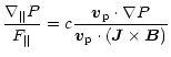 |
(C.1) | |
| = | (C.2) |
In Fig. C.1 we plot the worst case of cold fluid
violation and best case of cold fluid validity. Again the worst case
appears at lower accretion rates and in outer wind zones. It can be
seen that high values of
![]() and
and
![]() can be
attained, hinting at the importance of gas heating on jet dynamics
(providing both enthalpy at the base of the jet and/or pressure
support against recollimation further out). We underline that models
inconsistent with the cold fluid approximation are those found to have
the largest difficulty in meeting the observations
(Paper II). Conversely, models that better reproduce
observations also fulfill the cold fluid approximation. For those
models, the thermal pressure gradient appears to be fairly negligible
with respect to the Lorentz force.
can be
attained, hinting at the importance of gas heating on jet dynamics
(providing both enthalpy at the base of the jet and/or pressure
support against recollimation further out). We underline that models
inconsistent with the cold fluid approximation are those found to have
the largest difficulty in meeting the observations
(Paper II). Conversely, models that better reproduce
observations also fulfill the cold fluid approximation. For those
models, the thermal pressure gradient appears to be fairly negligible
with respect to the Lorentz force.
The first ignored process is the term
![]() .
This term decreases for increasing accretion rate and
.
This term decreases for increasing accretion rate and
![]() due to the lower ionizations found in these regions. It is
plotted in Fig. C.2 for the worst case (model C,
due to the lower ionizations found in these regions. It is
plotted in Fig. C.2 for the worst case (model C,
![]() and
and
![]() AU). There, it reaches at most
AU). There, it reaches at most ![]() 13% of
13% of
![]() .
Typical values for higher accretion rates are
only
.
Typical values for higher accretion rates are
only ![]() 0.1% of
0.1% of
![]() .
.
Next we consider heating/cooling of the gas by collision with dust
grains, given by Hollenbach & McKee (1979):
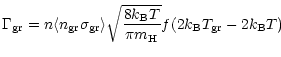 |
(C.3) |
| (C.4) |
Heating due to cosmic rays, which could be important in the outer
tenuous zones of the wind is (Spitzer & Tomasko 1968),
| (C.5) |
Formally, our temperature integration is an initial value problem. In the absence of a self-consistent description of the disc thermodynamics, there is some freedom in the initial temperature determination. It is therefore crucial to check that the subsequent thermal evolution of the wind does not depend critically on the adopted initial value.
Safier obtained the initial temperature by assuming
the poloidal velocity at the slow magnetosonic point (
![]() )
to be the sound speed for adiabatic perturbations
)
to be the sound speed for adiabatic perturbations
![]() .
Here, we have chosen
to compute the initial temperature assuming local thermal equilibrium
.
Here, we have chosen
to compute the initial temperature assuming local thermal equilibrium
![]() .
Our method produces lower initial temperatures than
Safier due to adiabatic cooling.
.
Our method produces lower initial temperatures than
Safier due to adiabatic cooling.
For high accretion rates
![]() our initial temperature versus
our initial temperature versus ![]() has a
minimum at the beginning of the dusty zone: inside the sublimation
cavity, the thermal equilibrium is between photoionization heating and
adiabatic cooling. Just beyond the dust sublimation radius,
photoionization heating is strongly reduced, but the ionization
fraction is still too high for efficient drag heating, resulting in a
low initial equilibrium temperature.
has a
minimum at the beginning of the dusty zone: inside the sublimation
cavity, the thermal equilibrium is between photoionization heating and
adiabatic cooling. Just beyond the dust sublimation radius,
photoionization heating is strongly reduced, but the ionization
fraction is still too high for efficient drag heating, resulting in a
low initial equilibrium temperature.
The initial ionization fraction is similarly determined by assuming
local ionization equilibrium
![]() for all elements. It
decreases with
for all elements. It
decreases with ![]() .
For
.
For
![]() and
and
![]() AU, the initial ionization
fraction is set to a minimum value by assuming that Na is fully
ionized, which is somewhat arbitrary. However, as gas is lifted up
above the disk plane, the dust opacity decreases and the gas heats up,
so that ionization becomes dominated by other photoionized heavy
species and by protons, all computed self consistently.
AU, the initial ionization
fraction is set to a minimum value by assuming that Na is fully
ionized, which is somewhat arbitrary. However, as gas is lifted up
above the disk plane, the dust opacity decreases and the gas heats up,
so that ionization becomes dominated by other photoionized heavy
species and by protons, all computed self consistently.
In order to check that our results do not depend on the initial temperature, we have run model B for a broad range of initial temperatures. As shown in Fig. C.3), we find that the thermal and ionization evolution quickly becomes insensitive to the initial temperature. If we start with a temperature lower than the local isothermal condition, the dominant adiabatic cooling is strongly reduced, and the gas strongly heats up, quickly converging to our nominal curve. If we start with a higher initial temperature, adiabatic cooling is stronger, and we have the characteristic dip in the temperature found by Safier. Our choice of initial temperature has the advantage of reducing this dip, which is somewhat artificial (see Fig. C.3). In either case, we conclude that our results are robust with respect to the choice of initial temperature. In particular, the distance at which the hot plateau is reached, which has a crucial effect on line profile predictions, is unaffected.
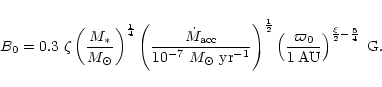
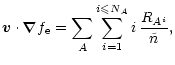

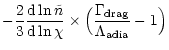
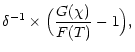
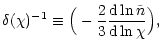
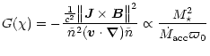

![\begin{figure}
\par\includegraphics[width=8.8cm,clip]{figb1.epsi} \end{figure}](/articles/aa/full/2001/38/aa1260/img353.gif)
![\begin{figure}
\par\includegraphics[width=6.8cm,clip]{figc1.epsi} %
\end{figure}](/articles/aa/full/2001/38/aa1260/img387.gif)
![\begin{figure}
\par\includegraphics[angle=-90,width=8.8cm,clip]{figc2.epsi} %
\end{figure}](/articles/aa/full/2001/38/aa1260/img407.gif)
![\begin{figure}
\par\includegraphics[width=8.8cm,clip]{figc3.epsi}\end{figure}](/articles/aa/full/2001/38/aa1260/img424.gif)