A&A 377, 23-43 (2001)
DOI: 10.1051/0004-6361:20010862
Binary black holes and tori in AGN
I. Ejection of stars and merging of the binary
C. Zier
-
P. L. Biermann
Max-Planck-Institut für Radiostronomie (MPIfR)
Auf dem Hügel 69, 53121 Bonn, Germany
Received 2 March 2001 / Accepted 14 June 2001
Abstract
Observations of HST and groundbased data strongly suggest that most
galaxies harbour central supermassive black holes and that most
galaxies merge
with others. Consequently a black hole binary emerges as the two black
holes are spiraling into the center towards each other. In our work we
are investigating two basic questions of our understanding of the
central activity of galaxies and find that both can be answered with
``yes'': (1) Do the black holes actually merge?
(2) And does the effect of the torque of the black hole binary on the
surrounding stellar distribution help to explain the presence of the
ubiquitous torus of molecular material surrounding apparently all
active galactic nuclei?
The first question is the topic of the present
article, while the second question will be subject of a subsequent
paper.
Simulating the evolution of a stellar cluster in the potential of such
a binary by solving the equations of the restricted three body problem
we obtained the following results: provided that the cluster is
about as massive as the black hole binary the two black holes coalesce
after
 due to ejection of stars and finally via
emission of gravitational radiation. Whether a star is ejected or
not crucially depends on its angular momentum. Almost all stars
whose angular momentum is twice as large as that of a star circulating
around the binary in
a distance corresponding to that between the black holes, stay
bound to the binary.
In a sequence of models where the mass of the secondary black hole
increases while M1 is
fixed, a bigger fraction of stars is ejected. For a more massive
binary also the cluster has to be more massive in order to allow the
two black holes to coalesce. The merger then proceeds on smaller time
scales.
The cluster is depleted in the central region and the final
distribution of stars assumes a torus-like structure, peaking at
three times the initial distance of the two black holes. The
relationship of the bound stars to the obscuring torus in active
galactic nuclei will be investigated in a subsequent paper.
due to ejection of stars and finally via
emission of gravitational radiation. Whether a star is ejected or
not crucially depends on its angular momentum. Almost all stars
whose angular momentum is twice as large as that of a star circulating
around the binary in
a distance corresponding to that between the black holes, stay
bound to the binary.
In a sequence of models where the mass of the secondary black hole
increases while M1 is
fixed, a bigger fraction of stars is ejected. For a more massive
binary also the cluster has to be more massive in order to allow the
two black holes to coalesce. The merger then proceeds on smaller time
scales.
The cluster is depleted in the central region and the final
distribution of stars assumes a torus-like structure, peaking at
three times the initial distance of the two black holes. The
relationship of the bound stars to the obscuring torus in active
galactic nuclei will be investigated in a subsequent paper.
Key words: galaxies: active -
galaxies: nuclei -
galaxies: interactions -
galaxies: kinematics and dynamics
The bright radiation in the centers of galaxies is generally thought to
be produced by a powerful engine, which is located at the dynamical
center of its host. Because the region from where this high luminosity
is emitted is concentrated to a small volume, non-stellar activity is
suspected to cause such a great energy output. It is argued that these
active galactic nuclei (AGN) are powered by accretion onto a massive
black hole (BH) in the center. While matter is sinking down in the
potential of such a black hole, energy is released and this accretion
process is thought to be dominated by an accretion disk.
The maximum mass of
these central objects, of order 10-2.5 times the stellar
spheroidal mass of their host galaxies
(Magorrian et al. 1998; Richstone et al. 1998; Wang & Biermann 1998; Macchetto 1999), is
consistent with the mass in black holes needed to produce the
observed energy density in quasar light if reasonable assumptions are
made about the efficiency of the energy production of the nucleus
(Novikov & Thorne 1972; Shakura & Sunyaev 1973; Chokshi & Turner 1992; Blandford 1999).
One of the best candidates of galaxies showing strong evidence for
harbouring a massive BH in its center is NGC 4258.
From VLBI observations of megamasers in its nucleus,
Miyoshi et al. (1995) deduce the existence of a mass of
about
 which must be located inside the inner
radius of
which must be located inside the inner
radius of
 .
Peterson & Wandel (1999) use emission-line variability
data on NGC 5548, a Seyfert 1 galaxy, to infer the existence of a
mass of order
.
Peterson & Wandel (1999) use emission-line variability
data on NGC 5548, a Seyfert 1 galaxy, to infer the existence of a
mass of order
 within the inner few light days
of the nucleus. There are numerous other examples suggesting that most
galaxies keep a super-massive black hole in their center. This is
the first of our two basic assumptions.
within the inner few light days
of the nucleus. There are numerous other examples suggesting that most
galaxies keep a super-massive black hole in their center. This is
the first of our two basic assumptions.
According to hierarchical models a typical bright galaxy has merged a
few times since the quasar era
(Frenk et al. 1988; Carlberg & Couchman 1989; Baugh et al. 1996; Richstone et al. 1998).
For binary black holes with
 the timescales
for a decay in the different regimes indicate that the binary will merge
on a scale short compared to the time when the next merger event
occurs (Xu & Ostrike 1994). The rate of mergers for bright galaxies in the
observable universe may exceed
the timescales
for a decay in the different regimes indicate that the binary will merge
on a scale short compared to the time when the next merger event
occurs (Xu & Ostrike 1994). The rate of mergers for bright galaxies in the
observable universe may exceed
 (Richstone et al. 1998). Taking
into
account that local quasars might have been formed by major mergers
between galaxies, Taniguchi (1999) proposes that all
active galactic nuclei of the local universe are products either from
minor or major mergers. This appears to be consistent
with almost all important observational properties of Seyfert galaxies.
Recent studies (Mulchaey & Regan 1997; Ho et al. 1997; de Robertis et al. 1998) show
that Seyfert galaxies do not have always either bar-structure or companion
galaxies, what often had been considered to be the cause of effective
gas fuelling to the central engine
(see, e.g., Adams 1977; Noguchi 1988;
Shlosman et al. 1990; Barnes & Hernquist 1992).
An alternative way to supply the central engine with matter is the
merger driven fuelling, see for example
Toomre & Toomre (1972), Roos (1981), Mihos & Hernquist (1994), de Robertis et al. (1998).
In order to complete a minor merger about
(Richstone et al. 1998). Taking
into
account that local quasars might have been formed by major mergers
between galaxies, Taniguchi (1999) proposes that all
active galactic nuclei of the local universe are products either from
minor or major mergers. This appears to be consistent
with almost all important observational properties of Seyfert galaxies.
Recent studies (Mulchaey & Regan 1997; Ho et al. 1997; de Robertis et al. 1998) show
that Seyfert galaxies do not have always either bar-structure or companion
galaxies, what often had been considered to be the cause of effective
gas fuelling to the central engine
(see, e.g., Adams 1977; Noguchi 1988;
Shlosman et al. 1990; Barnes & Hernquist 1992).
An alternative way to supply the central engine with matter is the
merger driven fuelling, see for example
Toomre & Toomre (1972), Roos (1981), Mihos & Hernquist (1994), de Robertis et al. (1998).
In order to complete a minor merger about
 are needed. This
is enough time to smear out the relics so that most of the advanced
minor mergers may be observed as ordinary-looking isolated galaxies
(Walker et al. 1996) and Seyfert galaxies are observed to possess a
statistically significant excess of
faint (
are needed. This
is enough time to smear out the relics so that most of the advanced
minor mergers may be observed as ordinary-looking isolated galaxies
(Walker et al. 1996) and Seyfert galaxies are observed to possess a
statistically significant excess of
faint (
 )
companion galaxies (Fuentes-Williams & Stocke 1988).
The frequent merging of galaxies is our second basic assumption and
consequently leads to massive black hole binaries in combination
with the first assumption.
)
companion galaxies (Fuentes-Williams & Stocke 1988).
The frequent merging of galaxies is our second basic assumption and
consequently leads to massive black hole binaries in combination
with the first assumption.
Observations show that all
ellipticals have central density cusps which can be divided into
"weak'' cusps (
 ,
bright ellipticals) and
"strong'' (
,
bright ellipticals) and
"strong'' (
 ,
fainter ellipticals) cusps
(Kormendy et al. 1994; Kormendy et al. 1996; Faber 1997).
It has already been suggested by Begelman et al. (1980) that the mass
ejection due the merging of two
massive black holes should reduce the central density and that the core
expands. In several numerical simulations it has been found that
the merging of two galaxies and their central black holes can account for
the weak cusps, where the sinking of the BH is the dominant
mechanism (Makino & Ebisuzaki 1996; Nakano & Makino 1999; Milosavljevic & Merritt 2001).
,
fainter ellipticals) cusps
(Kormendy et al. 1994; Kormendy et al. 1996; Faber 1997).
It has already been suggested by Begelman et al. (1980) that the mass
ejection due the merging of two
massive black holes should reduce the central density and that the core
expands. In several numerical simulations it has been found that
the merging of two galaxies and their central black holes can account for
the weak cusps, where the sinking of the BH is the dominant
mechanism (Makino & Ebisuzaki 1996; Nakano & Makino 1999; Milosavljevic & Merritt 2001).
Because the critical central regions of AGN are strongly
nonspherical but spatially unresolved, orientation effects are
thought to be important, see e.g. the discussion of
quasar spectra by Sanders et al. (1989). Thus the same object seen from
other angles would be classified differently. In type 1 objects
the radiation emerging from the center is not blocked by matter in
the line of sight of the observer. Hence the X-rays in the  -range, the big blue bump (BBB) and the broad emission line
region (BLR) as
well as the narrow emission line region (NLR) can be seen directly. On
the other hand, objects classified as type 2, show strongly absorbed
X-rays and no clear evidence for the big blue bump and the BLR
(Lawrence & Elvis 1982). But
the NLR is indistinguishable from that detected in type 1
objects. This region is located at bigger radii from the center
and thus not blocked by matter at a smaller distance in the line of
sight. Sometimes a
type 1 spectrum is seen in the polarized light of type 2 classified
objects and thus gives strong evidence for the existence of an obscuring
torus, see e.g. Miller et al. (1991): this is interpreted within the
unification model as radiation
emerging from the center and then scattered by ionized matter in the
opening of the torus into the line of sight
(Antonucci & Miller 1985; Miller & Goodrich 1990; Tran & Kay 1992). This model ascribes the
different appearance of AGN rather to different orientations than to
intrinsic differences. Its basic ingredients which are responsible
for the non-spherical symmetry of the nucleus are relativistic
beaming in a jet, the obscuration of the central engine by a
molecular, dusty torus, and possibly the power of the central
engine (see e.g the reviews by
Antonucci 1993; Urry & Padovani 1995; Madejski 1998; 1999 and articles by
Falcke & Biermann 1995; Falcke et al. 1995; Taniguchi 1999; 2000).
Recent XMM-Newton observations of the radio-quiet quasar Mrk 205
might provide the first evidence for a dust-torus in a quasar
(Reeves et al. 2001). XMM-data of IRAS 13349+2438 suggest
column-densities which are consistent with a dusty torus
(Sako et al. 2001).
Observations impose important constraints on the
properties of such tori. From X-ray absorption a
column density of
-range, the big blue bump (BBB) and the broad emission line
region (BLR) as
well as the narrow emission line region (NLR) can be seen directly. On
the other hand, objects classified as type 2, show strongly absorbed
X-rays and no clear evidence for the big blue bump and the BLR
(Lawrence & Elvis 1982). But
the NLR is indistinguishable from that detected in type 1
objects. This region is located at bigger radii from the center
and thus not blocked by matter at a smaller distance in the line of
sight. Sometimes a
type 1 spectrum is seen in the polarized light of type 2 classified
objects and thus gives strong evidence for the existence of an obscuring
torus, see e.g. Miller et al. (1991): this is interpreted within the
unification model as radiation
emerging from the center and then scattered by ionized matter in the
opening of the torus into the line of sight
(Antonucci & Miller 1985; Miller & Goodrich 1990; Tran & Kay 1992). This model ascribes the
different appearance of AGN rather to different orientations than to
intrinsic differences. Its basic ingredients which are responsible
for the non-spherical symmetry of the nucleus are relativistic
beaming in a jet, the obscuration of the central engine by a
molecular, dusty torus, and possibly the power of the central
engine (see e.g the reviews by
Antonucci 1993; Urry & Padovani 1995; Madejski 1998; 1999 and articles by
Falcke & Biermann 1995; Falcke et al. 1995; Taniguchi 1999; 2000).
Recent XMM-Newton observations of the radio-quiet quasar Mrk 205
might provide the first evidence for a dust-torus in a quasar
(Reeves et al. 2001). XMM-data of IRAS 13349+2438 suggest
column-densities which are consistent with a dusty torus
(Sako et al. 2001).
Observations impose important constraints on the
properties of such tori. From X-ray absorption a
column density of
 is
deduced (Mushotzky 1982; Mulchaey et al. 1992; Madejski 1998),
i.e. the tori have to be optically
thick. Number ratios of types 1 and 2 objects tell us that such tori
are also geometrically thick (see e.g. Taniguchi & Anabuki 1999 and
references therein). The AGN spectra also show a prominent infrared
bump between
is
deduced (Mushotzky 1982; Mulchaey et al. 1992; Madejski 1998),
i.e. the tori have to be optically
thick. Number ratios of types 1 and 2 objects tell us that such tori
are also geometrically thick (see e.g. Taniguchi & Anabuki 1999 and
references therein). The AGN spectra also show a prominent infrared
bump between
 and
and
 (Sanders et al. 1989), which is thought to be generated by dust
reprocessing the incident radiation from the center. In about
(Sanders et al. 1989), which is thought to be generated by dust
reprocessing the incident radiation from the center. In about
 distance the dust in the torus is heated to its
evaporation temperature of about
distance the dust in the torus is heated to its
evaporation temperature of about
 and then reemitting
the central ratiation in the infrared
(Sanders et al. 1989; Haas et al. 2000). Pier & Krolik (1992) and Pier & Krolik (1993) find
that a very compact and thick dust torus, supported by radiation
pressure, is not able to provide the
required broad temperature range of the dust in order to explain the
infrared (IR) emission. But a clumpy torus, as
suggested by Krolik & Begelman (1988), has the advantage that the dust,
when organized in clouds, can survive more easily the strong
radiation field of the AGN. Also the dust in the outer parts can be
heated to higher temperatures and a broader temperature range can be
achieved (Efstathiou & Rowan-Robinson 1995). Such a clumpy torus
model seems to be the most promising scenario also to
Haas et al. (2000). A torus is also used in high energy physics
according to Protheroe & Biermann (1997) who show for Blazars
that the TeV
and then reemitting
the central ratiation in the infrared
(Sanders et al. 1989; Haas et al. 2000). Pier & Krolik (1992) and Pier & Krolik (1993) find
that a very compact and thick dust torus, supported by radiation
pressure, is not able to provide the
required broad temperature range of the dust in order to explain the
infrared (IR) emission. But a clumpy torus, as
suggested by Krolik & Begelman (1988), has the advantage that the dust,
when organized in clouds, can survive more easily the strong
radiation field of the AGN. Also the dust in the outer parts can be
heated to higher temperatures and a broader temperature range can be
achieved (Efstathiou & Rowan-Robinson 1995). Such a clumpy torus
model seems to be the most promising scenario also to
Haas et al. (2000). A torus is also used in high energy physics
according to Protheroe & Biermann (1997) who show for Blazars
that the TeV  -emission site is far from the central engine
due to
-emission site is far from the central engine
due to
 -interactions with the far infrared photon
field of the torus.
-interactions with the far infrared photon
field of the torus.
Now, based on our two underlying assumptions, necessarily leading to a
black hole binary, we here investigate the influence of a stellar
cluster and a black hole binary (BHB) in its center on each other in
order to answer two basic questions in our understanding of the
central activity of galaxies:
- Do the two black holes in the center of two colliding galaxies
actually merge?
- Does the effect of the torque of the binary black holes on the
stellar distribution help to explain the presence of the ubiquituous
torus of molecular material surrounding apparently all active galactic
nuclei (AGN) in the "unified scheme''?
Since a BHB has a non-spherical symmetry it might cause an
initially spherical symmetric stellar distribution to possibly
assume a torus-like structure.
Hence, to find an answer to both the questions we performed numerical
simulations of the stars in
the potential of the BHB by solving the three-body problem for each
star of the initial distribution. Integrating over all stars of the
cluster we obtain the properties of the stellar
population and can trail its evolution under the influence of the
binary.
Following the suggestion by Kazanas (1989),
Alexander & Netzer (1994) and Alexander & Netzer (1997) that the
BLR is made up by stars and their winds, we propose that the gas and
dust of the torus is bound to the stars within their winds. The
dynamics of these stars in the potential of the binary then supports
the torus in the vertical direction, solving the problem of how to
keep the torus geometrically thick.
In this paper we investigate the conditions for which the black holes merge
and how long such a merger lasts.
We will first use a mass-ratio of q=10 for the black holes to
discuss the results in more detail. Afterwards we compare them with
those obtained for the ratios q=1 and 100.
In a following paper (Paper II) we will concentrate on the
configuration of the stars remaining bound to the black holes, their
ability to constitute a dusty torus and the observational consequences
in order to answer the second question.
The evolution of the orbit of a comparatively low mass
secondary black hole moving around a massive BH M1in the center of a massive galaxy is investigated with
analytical and numerical means by Polnarev & Rees (1994).
Dynamical friction between both
galaxies results in a loss of energy and angular momentum so that the
cores of the galaxies quickly approach each other. The
probability of merging with a given initial value of pericenter is
roughly proportional to the square of this value. Thus small initial
pericenters are unlikely and in the
most cases Polnarev & Rees (1994) find the eccentricity
never to exceed a value of order 0.1. After the stars surrounding
the secondary black hole have been
stripped off by tidal effects, it moves on bound
orbits in the mean gravitational field of the core of the primary
galaxy. Dynamical friction extracts kinetic energy from
the secondary BH (Chandrasekhar 1943; Binney & Tremaine 1987) which binds to M1at the radius
 .
Below this
separation M2 is still surrounded by the sea of field stars of the
core. The density enhancement of surrounding stars in its wake after
gravitational interaction further decreases the velocity of M2 so
that it keeps on spiralling inwards due to
dynamical friction. The kinetic energy is lost to these stars,
resulting in a heating of the core, but the stars do not gain enough
energy as to leave the system. Eventually, after some
.
Below this
separation M2 is still surrounded by the sea of field stars of the
core. The density enhancement of surrounding stars in its wake after
gravitational interaction further decreases the velocity of M2 so
that it keeps on spiralling inwards due to
dynamical friction. The kinetic energy is lost to these stars,
resulting in a heating of the core, but the stars do not gain enough
energy as to leave the system. Eventually, after some
 ,
the distance between both the BHs
shrinks to the cusp-radius of M1,
,
the distance between both the BHs
shrinks to the cusp-radius of M1,
 ,
where the velocity dispersion of the stars of the core
equals the keplerian velocity in the potential of M1(Begelman et al. 1980; Mikkola & Valtonen 1992; Vecchio et al. 1994; Quinlan 1996). Inside
,
where the velocity dispersion of the stars of the core
equals the keplerian velocity in the potential of M1(Begelman et al. 1980; Mikkola & Valtonen 1992; Vecchio et al. 1994; Quinlan 1996). Inside
 the kinematics of the stars and M2 is dominated by
the potential of M1, and the stars are now interacting with both
BHs rather than with M2 only. This is the point where we start our
calculations. Neglecting the influence of the other
stars of the core we are now dealing with the three-body problem for a
single
star in the potential of both BHs. In the interaction with the black
hole binary (BHB) some stars gain enough energy in order to be ejected
from the central region. On the other hand the more distant stars just
perturb the binary's center of mass and leave its semi-major axis
unaffected and the ejection of individual stars becomes the
dominant process for further hardening. Thus stars moving on orbits
with radii of about the semi-major axis of the binary contribute most
to the shrinking of the binary in this stage. This is also found by
Hemsendorf et al. (2001) in their numerical calculations. If there are sufficient
such stars the hardening continues till eventually the black holes
coalesce due to the emission of gravitational radiation. Otherwise the
hardening stalls if the inner region is not sufficiently refilled with
matter by some other process.
the kinematics of the stars and M2 is dominated by
the potential of M1, and the stars are now interacting with both
BHs rather than with M2 only. This is the point where we start our
calculations. Neglecting the influence of the other
stars of the core we are now dealing with the three-body problem for a
single
star in the potential of both BHs. In the interaction with the black
hole binary (BHB) some stars gain enough energy in order to be ejected
from the central region. On the other hand the more distant stars just
perturb the binary's center of mass and leave its semi-major axis
unaffected and the ejection of individual stars becomes the
dominant process for further hardening. Thus stars moving on orbits
with radii of about the semi-major axis of the binary contribute most
to the shrinking of the binary in this stage. This is also found by
Hemsendorf et al. (2001) in their numerical calculations. If there are sufficient
such stars the hardening continues till eventually the black holes
coalesce due to the emission of gravitational radiation. Otherwise the
hardening stalls if the inner region is not sufficiently refilled with
matter by some other process.
Therefore, once the black holes approached each other as close as the cusp
radius, the eccentricity of their orbits is likely to be very small
(Milosavljevic & Merritt 2001) so that we assume them to move on circular orbits
around each other.
2.1 Collisionless systems
The net force acting on a star
in a galaxy is mainly determined by the large structure of the galaxy.
Consequently the gravitational force of the mass distribution in the
galaxy varies smoothly with space as it acts on a single star.
The number
 ,
how often an individual star of mass mhas to cross
a system of N identical stars so that the stars velocity v is changed
by order of itself is
,
how often an individual star of mass mhas to cross
a system of N identical stars so that the stars velocity v is changed
by order of itself is
 |
|
|
(1) |
The parameter  may be
written as
may be
written as
 ,
see Binney & Tremaine (1987).
The largest possible impact parameter is limited by the
scale R of the stellar distribution. If, on the other hand, the impact
parameter falls below the limit
,
see Binney & Tremaine (1987).
The largest possible impact parameter is limited by the
scale R of the stellar distribution. If, on the other hand, the impact
parameter falls below the limit
 the
assumption of nearly a straight-line trajectory, made to obtain expression
(1), breaks down.
the
assumption of nearly a straight-line trajectory, made to obtain expression
(1), breaks down.
The time a star needs to cross the volume of the stellar
distribution is of order
 so that the relaxation
time may be defined as
so that the relaxation
time may be defined as
 .
Now, for a total amount of N=108 solar mass stars we obtain for the
number of crossing times
.
Now, for a total amount of N=108 solar mass stars we obtain for the
number of crossing times
 .
If we assume the star to be of
solar mass and the cluster to extend to radii of
.
If we assume the star to be of
solar mass and the cluster to extend to radii of
 we
obtain the typical velocity of a star to be
we
obtain the typical velocity of a star to be
 .
This allows to compute the relaxation time,
which is
.
This allows to compute the relaxation time,
which is
 .
.
Thus, compared to the trajectory a star would follow if the other matter
would be perfectly smoothly distributed, individual stellar encounters
perturb this trajectory only over of order
 crossing
times. This means that it takes several crossing times to deflect a
star from
its mean trajectory and therefore it is possible to obtain some
understanding of the dynamics by investigating the orbits of the stars
in a suitable mean potential without taking into account individual
stellar encounters. Since the time range of our simulation is smaller by a
factor of
crossing
times. This means that it takes several crossing times to deflect a
star from
its mean trajectory and therefore it is possible to obtain some
understanding of the dynamics by investigating the orbits of the stars
in a suitable mean potential without taking into account individual
stellar encounters. Since the time range of our simulation is smaller by a
factor of  than the relaxation time we can neglect
individual stellar encounters in our calculations.
Thus the evolution of a stellar distribution in the potential of
a BHB can be modelled by solving the equations of motion of the
individual stars of a cluster separately. Afterwards the
results of the single stars can be combined to model the evolution
of the complete cluster.
than the relaxation time we can neglect
individual stellar encounters in our calculations.
Thus the evolution of a stellar distribution in the potential of
a BHB can be modelled by solving the equations of motion of the
individual stars of a cluster separately. Afterwards the
results of the single stars can be combined to model the evolution
of the complete cluster.
If we assume that the potential in the central region is dominated by
the two black holes we can neglect the mean potential of the stellar
distribution when we are solving the equations of motion for the
stars. Since the cluster can be
treated as a collisionless system, we can solve the equations of motion
for each star separately, i.e. we are
dealing with the restricted three body problem.
In the following all coordinates are given relative to the center of
mass, which is identified with the origin of the coordinate
system. The axis of rotation is the z-axis and
we always assume
 and correspondingly for the mass-ratio
 .
The two black holes are moving on circular orbits around each other in a
fixed distance of
.
The two black holes are moving on circular orbits around each other in a
fixed distance of
 .
.
To write the equations of motion in a dimensionless form we
used the following normalization constants
with the mass of the primary BH M1 being fixed to
 (see Appendix A).
 is
the dimensionless mass of the primary BH in units of
108 solar masses and equal to one throughout this paper.
The quantities
is
the dimensionless mass of the primary BH in units of
108 solar masses and equal to one throughout this paper.
The quantities
 and
and
 denote the dimensionless
distance between the BHs and the radial distance to the center of mass
respectively, both scaled to one parsec. In the following
we indicate dimensionless quantities with a tilde "
denote the dimensionless
distance between the BHs and the radial distance to the center of mass
respectively, both scaled to one parsec. In the following
we indicate dimensionless quantities with a tilde "
 ''
on top.
''
on top.
The numerical integration of the equations is processed faster
in the comoving frame where the BH masses are stationary on the
x-axis and the rotation axis is pointing along the z-axis with the
z=0-plane being the equatorial plane of the BHs.
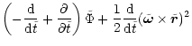
In this system the equations of motion read (see Appendix A):
These have been solved numerically after being supplied with a set of
initial conditions for the stars which we will discuss in the next
section.
In order to check the accuracy of the numerical integration, we keep
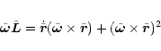
track of the deviations of the Jacobian Integral (Appendix
B), which is a conserved quantity in this problem.
The surface-brightness profiles of many elliptical galaxies are well
fitted by an isothermal sphere out to a few core radii. On the other
hand rotation curves of spiral galaxies are often remarkably flat out
to great radii, and this suggests that we should construct models that
deviate from the isothermal sphere only far from their cores
(Mihalas & Binney 1981; Binney & Tremaine 1987.
The structure of
an isothermal self-gravitating sphere of gas is identical with that
of a collisionless system of stars whose density in
phase-space is given by Eq. (C.4), see Appendix
C.
This correspondence between the gaseous and stellar-dynamical
isothermal sphere originates in the velocity distribution of both
systems. Integrating Eq. (C.4) over the
volume yields the Maxwell-Boltzmann distribution for the
velocities. As we know from kinetic gas
theory this is the equilibrium distribution for a gas
whose particles are allowed to collide elastically with each
other. Therefore, if a system of particles is described by a
distribution function
according to Eq. (C.4), it makes no difference whether
the particles collide with each other or not. This makes the
isothermal sphere a very well suited initial distribution for our
purposes.
The mean and the mean-square velocity of the stars in the isothermal
sphere,
 and
and
 ,
are independent of the position. Since the velocity
dispersion is isotropic everywhere its
components are the same:
,
are independent of the position. Since the velocity
dispersion is isotropic everywhere its
components are the same:
 .
.
Interestingly Milosavljevic & Merritt (2001) find in their numerical calculations
that the radial density profiles of the pre-merger galaxies and of the
merged galaxy just after the formation of a hard BHB are essentially
the same for a short time. For the initial density distribution
they used a powerlaw with index -2.
In our model we distribute the stars according to
the singular isothermal sphere (Eq. (C.9)) in
the range
 .
In order to obtain the
Maxwell-Boltzmann distribution in velocity each component has been
distributed according to a Gaussian.
Since we are interested in stars which initially are
bound by the potential of the BHB (E<0) and do not leave the system
immediately after the calculations started we choose the free
parameter
.
In order to obtain the
Maxwell-Boltzmann distribution in velocity each component has been
distributed according to a Gaussian.
Since we are interested in stars which initially are
bound by the potential of the BHB (E<0) and do not leave the system
immediately after the calculations started we choose the free
parameter  ,
the velocity dispersion, to be a third of the
escape velocity,
,
the velocity dispersion, to be a third of the
escape velocity,
 .
.
The initial conditions for 8000 stars have been generated
and supplied to Eqs. (3). These are solved with a Runge-Kutta code of
fourth order based on the routine rkck by
Press et al. (1995). The stepsize is selfadapting to ensure
that the desired
accuracy is always maintained and that the stepsize does not become
too small in order to save computing time. Due to our choice of the
initial conditions all stars are bound to the binary in the beginning,
having negative energies.
Some of them are ejected later during the run time. We
define a star as being ejected if the following three conditions are
fulfilled simultaneously:
- the energy of the star is positive
 ;
;
- its radial distance in orbit is bigger than
 ;
;
- the radial velocity component is positive
 .
.
The simulation is stopped after the time
 (in dimensionless units) is reached or if the star has been
ejected before.
(in dimensionless units) is reached or if the star has been
ejected before.
 corresponds to about
  revolutions of the BHB or to
 .
.
In the next section we present the results we obtained for the
simulation using a mass-ratio q=10 (
 ). Afterwards
we will compare them with the results we obtained for q=1 and
q=100.
). Afterwards
we will compare them with the results we obtained for q=1 and
q=100.
![\begin{figure}
\includegraphics[width=85mm]{h2731f1.eps}\end{figure}](/articles/aa/full/2001/37/aah2731/Timg107.gif) |
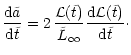
Figure 1:
Initially the central region is dominated by the ejected population
(EP), the outer regions by the bound population (BP). Finally, at
,
the bound star distribution follows a powerlaw
with index -4 in the heated region (
 ), while an index ), while an index  is maintained in the
range
is maintained in the
range
 .
The inner parts are scoured
out and a maximum emerges at .
The inner parts are scoured
out and a maximum emerges at
 ,
showing the
torus-like configuration the stars assume. For ,
showing the
torus-like configuration the stars assume. For
 a cusp of stars bound to M1 only is left. a cusp of stars bound to M1 only is left.  is
normalized to
and
is
normalized to
and
 such that the area
underneath the solid line is 1.
such that the area
underneath the solid line is 1. |
| Open with DEXTER |
In the following all quantities are given in and related to the
observers frame if not indicated otherwise. The origin of the
coordinate system is the center of mass of the BHB, with its rotation
axis pointing along the z-axis. At
 both black holes lie on
the x-axis, with M1 situated on the positive and M2 on the
negative seminaxis. The y-axis is perpendicular to both the others
so that all axes form a right handed tripod.
In spherical coordinates
both black holes lie on
the x-axis, with M1 situated on the positive and M2 on the
negative seminaxis. The y-axis is perpendicular to both the others
so that all axes form a right handed tripod.
In spherical coordinates  denotes the angle to the positive
z-axis, and
denotes the angle to the positive
z-axis, and  is the azimuth in the x-y plane.
A key feature is the torque exerted by the rotating black holes on the
stars, which changes the star's orbit and can eject it from the
system.
During the simulation we kept track of the single stars what enables
us at all times to assign them either to the ejected population (EP),
which is constituted
by stars being ejected before the end of the simulation, or to the
bound population (BP) when they remain tied to the binary.
Both these populations combine to
give the "total population'' (TP). Quantities referring to EP, BP and TP are
denoted with the indices "ej'', "bn'' and "total'' respectively.
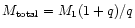
![\begin{figure}
\par\mbox{\includegraphics[angle =-90,width=73mm]{H2731_02.eps}\h...
...s}\hspace{2.4cm}
\includegraphics[width=74.5mm]{H2731_07.eps} }
\par\end{figure}](/articles/aa/full/2001/37/aah2731/Timg118.gif) |
Figure 2:
Cuts through the stellar density in the comoving frame are shown with
contours logarithmically scaled. The
right panel displays the equatorial plane (BHs marked by black spots).
Perpendicular to it the x=0-plane is shown (left panel), with
the y-axis drawn as dashed line, so that the BHs are in front and
behind the paper-plane. The
initial distribution is a Gaussian and the mass-ratio is
10. Time increases from top to bottom (indicated by
 ). After initially stars close to M2's orbit
( ). After initially stars close to M2's orbit
( 1 1 )
are ejected (2nd row) also the polar regions
are depleted and a torus in the equatorial plane finally emerges at )
are ejected (2nd row) also the polar regions
are depleted and a torus in the equatorial plane finally emerges at
 (3rd row).
 |
| Open with DEXTER |
3.1 The dynamics of the stars
The density distribution of both populations EP and BP shows that
the bound stars dominate the outer regions
(
 ,
dashed-dotted line in
Fig. 1). With decreasing radius the fraction of
ejected stars (long-dashed line) is increasing with both populations
being comparable in number density in a distance
,
dashed-dotted line in
Fig. 1). With decreasing radius the fraction of
ejected stars (long-dashed line) is increasing with both populations
being comparable in number density in a distance
 ,
corresponding to
,
corresponding to
 .
At
the density of the BP has a
maximum and after a gap in the distribution between 1 and
.
At
the density of the BP has a
maximum and after a gap in the distribution between 1 and
 ,
where M2 is circling around M1,
the density of bound stars is increasing again towards smaller
radii.
Niemeyer & Biermann (1993) could reproduce the range of observed mm to
infrared spectra of radio-weak quasars. In their model dust is
confined to molecular clouds in a disk configuration and is heated by
the central engine.
According to the model by Barvainis (1987) the dust is heated to
its evaporation temperature by the central UV luminosity in
,
where M2 is circling around M1,
the density of bound stars is increasing again towards smaller
radii.
Niemeyer & Biermann (1993) could reproduce the range of observed mm to
infrared spectra of radio-weak quasars. In their model dust is
confined to molecular clouds in a disk configuration and is heated by
the central engine.
According to the model by Barvainis (1987) the dust is heated to
its evaporation temperature by the central UV luminosity in
 distance. This evaporation radius is taken as the inner
radius of the torus by Lawrence (1991) and is in very good
agreement with the inner edge we find for the bound stellar
distribution at about
(Fig. 1).
Krolik & Begelman (1988) determine the inner radius of the
torus from the balance between cloud evaporation by central radiation
and inflow by dissipative processes in the torus and also obtain
.
At distances smaller than one parsec (
distance. This evaporation radius is taken as the inner
radius of the torus by Lawrence (1991) and is in very good
agreement with the inner edge we find for the bound stellar
distribution at about
(Fig. 1).
Krolik & Begelman (1988) determine the inner radius of the
torus from the balance between cloud evaporation by central radiation
and inflow by dissipative processes in the torus and also obtain
.
At distances smaller than one parsec (
 )
only 62 stars of the BP (a fraction of 1/80) are found at
.
These are bound to the primary black hole only, and
till the end of the simulation the number of stars in this cusp-region
is increased by just one which has been captured by M1.
)
only 62 stars of the BP (a fraction of 1/80) are found at
.
These are bound to the primary black hole only, and
till the end of the simulation the number of stars in this cusp-region
is increased by just one which has been captured by M1.
The evolution of the initial density distribution (a Gaussian) to its
final state is shown in Fig. 2. It displays cuts
through the 3-dimensional density distribution in the comoving frame
of the binary. The right panel shows the equatorial plane (z=0) with
the BHs
marked by the black points with white frames, M1 to the right. The
cuts in the left panel are perpendicular to the equatorial plane and
contain the x = 0-plane with the y-axis indicated by the dashed
line. The time proceeds from top to bottom and corresponds to
104.86, 106.57 and
 respectively for
q=10. The first row displays the distribution very close to
the initial state. After
respectively for
q=10. The first row displays the distribution very close to
the initial state. After
 (second row) we see that mainly stars close to the secondary's
orbit (
(second row) we see that mainly stars close to the secondary's
orbit (
 )
have been ejected and a gap appears at this
distance in the equatorial plane leaving a shell in the range
)
have been ejected and a gap appears at this
distance in the equatorial plane leaving a shell in the range
 behind. At about
 the
density has a maximum and
we can detect a shallow torus emerging at this radius. But still the
polar regions are populated as dense as the equatorial plane, see
Fig. 2, second row.
the
density has a maximum and
we can detect a shallow torus emerging at this radius. But still the
polar regions are populated as dense as the equatorial plane, see
Fig. 2, second row.
However, as is illustrated in the 3rd row of this figure, after
about
the central regions have been scoured out
and the hole in the distribution has a cylindrical geometry elongated
along the binaries rotation axis. In the equatorial plane finally a
torus with a radius of about
 emerges, showing that the
density distribution develops from the initial sphere over a
shell-like distribution (2nd row) to the final torus. Thus
one important condition of the unification scheme is fulfilled, namely
that the stars do assume a torus-like distribution at a distance which
is in agreement with the origin of thermal infrared emission by dust
(Barvainis 1987; Krolik & Begelman 1988; Haas et al. 2000). Whether this torus also satisfies
the other requirements, like optical thickness, will be investigated in
our Paper II.
emerges, showing that the
density distribution develops from the initial sphere over a
shell-like distribution (2nd row) to the final torus. Thus
one important condition of the unification scheme is fulfilled, namely
that the stars do assume a torus-like distribution at a distance which
is in agreement with the origin of thermal infrared emission by dust
(Barvainis 1987; Krolik & Begelman 1988; Haas et al. 2000). Whether this torus also satisfies
the other requirements, like optical thickness, will be investigated in
our Paper II.
![\begin{figure}
\par\includegraphics[width=8.8cm,clip]{fig3new.eps}\end{figure}](/articles/aa/full/2001/37/aah2731/Timg132.gif) |
Figure 3:
The component
 sin sin
 of the
normalized torque of the binary,
which acts on a star moving on a fixed circular orbit with radius
is displayed as function of time. The angle enclosed by
the rotation-axis of the binary and the orbital spin-axis of the star
is denoted by
and is varied in the range from
of the
normalized torque of the binary,
which acts on a star moving on a fixed circular orbit with radius
is displayed as function of time. The angle enclosed by
the rotation-axis of the binary and the orbital spin-axis of the star
is denoted by
and is varied in the range from  to
to
 .
Perturbations are stronger for orbits through the polar regions; these stronger
perturbations lead to secular changes in the orbit, finally leading to ejection for about half of the stars in the polar cap (see Fig. 2). .
Perturbations are stronger for orbits through the polar regions; these stronger
perturbations lead to secular changes in the orbit, finally leading to ejection for about half of the stars in the polar cap (see Fig. 2). |
| Open with DEXTER |
The basic topology of the final density distribution can be understood
in physical terms, where we consider the torque exerted by the two
black holes on an orbiting star.
Figure 3 shows of the normalized
torque the component
sin
relative to the z-axis of the BHB as a function of time for different angles
between the rotation axis of the BHB and the symmetry axis of
the star's orbit. The bigger
the angle
is (i.e. for orbits through the polar regions), the
more is the star's trajectory disturbed by the influence of the two BHs.
The curves are symmetric since
for simplicity
it has been assumed that the star is moving on a keplerian circle of
radius R around a point mass which corresponds to that of the binary
and is located at the origin. Of course real trajectories are
disturbed by the torque and the curves will not be symmetric any
more. The cumulative effect of these large excursions in the polarcap
regions deplete the stellar population leaving a torus behind.
Because of the conservation of the Jacobian Integral
(Eq. (B.4)) the stars which gain energy also gain angular
momentum in the z-component and thus help to enhance the density in
the equatorial plane.
In Paper II we will discuss the distribution of the BP and
investigate in the properties of the torus.
![\begin{figure}
\par\includegraphics[width=8.8cm,clip]{fig4new.eps}\end{figure}](/articles/aa/full/2001/37/aah2731/Timg133.gif) |
Figure 4:
The angular momentum clearly separates the BP (black dots) from the EP
(grey dots), which initially have less angular momentum.
The line of transition from the EP to the BP is drawn by eye.
Its almost constant value is decreasing with increasing mass-ratio
q. Along this line both populations diffuse into each other, showing
that the transition is smooth. |
| Open with DEXTER |
At
the finally ejected stars
can be clearly distinguished from the bound population by their total
angular momentum  or pericenter
 .
The mean
value of the angular momentum of the EP is smaller by a factor of
3.22 compared to
the BP (see Table 1). This
separation is clearly illustrated in Fig. 4, where
we have plotted the initial values of angular momentum of the stars
versus their radius.
The ejected stars, marked by grey dots, have low angular momenta,
while stars staying bound to the binary till the end of the simulation
(black dots) exceed a certain value. Both populations can be separated
from each other by a transition line, as seen in
Fig. 4.
The angular momentum has been normalized to the value of a star which
moves on circular orbits in a distance corresponding to the separation
of the BHs (
)
around the
combined mass of the BHs M1 + M1 which is situated at the center
(
.
The mean
value of the angular momentum of the EP is smaller by a factor of
3.22 compared to
the BP (see Table 1). This
separation is clearly illustrated in Fig. 4, where
we have plotted the initial values of angular momentum of the stars
versus their radius.
The ejected stars, marked by grey dots, have low angular momenta,
while stars staying bound to the binary till the end of the simulation
(black dots) exceed a certain value. Both populations can be separated
from each other by a transition line, as seen in
Fig. 4.
The angular momentum has been normalized to the value of a star which
moves on circular orbits in a distance corresponding to the separation
of the BHs (
)
around the
combined mass of the BHs M1 + M1 which is situated at the center
(
 ).
Along this transition-line, which is drawn by eye and
approaches a value of about 2 in these dimensionless units, the
different populations diffuse into each other so that the transition
from one population to the other is smooth.
).
Along this transition-line, which is drawn by eye and
approaches a value of about 2 in these dimensionless units, the
different populations diffuse into each other so that the transition
from one population to the other is smooth.
This value is double the angular momentum of a star moving on a circular
orbit with the radius corresponding to the separation of the
binary. Or, the other way round, this transition-value of corresponds to an orbit with a radius four times as big as the
semi-major axis of the binary.
![\begin{figure}
\par\includegraphics[width=8.8cm,clip]{fig5new.eps}\end{figure}](/articles/aa/full/2001/37/aah2731/Timg137.gif) |
Figure 5:
Ejected stars (grey dots) cover a region with  and and
 , marked by the horizontal and vertical
lines. This allows them to closely approach the orbit of M2. Bound
stars (black dots) avoid this unstable region. One unit corresponds to
. , marked by the horizontal and vertical
lines. This allows them to closely approach the orbit of M2. Bound
stars (black dots) avoid this unstable region. One unit corresponds to
. |
| Open with DEXTER |
However, due to their much lower angular momenta the finally ejected
stars come much closer to the black holes. For the mean pericenters we
get
 and
and
 showing
that they differ by more than a factor of 10.
In Fig. 5 we have plotted the initial
apocenters on the x-axis versus the initial pericenters on the
y-axis.
Without loss of information and to keep the figure distinct, we plotted
only 1/4 of each population, chosen by random. While the
pericenters of the ejected stars stay below
showing
that they differ by more than a factor of 10.
In Fig. 5 we have plotted the initial
apocenters on the x-axis versus the initial pericenters on the
y-axis.
Without loss of information and to keep the figure distinct, we plotted
only 1/4 of each population, chosen by random. While the
pericenters of the ejected stars stay below  (i.e.
,
horizontal line), their
apocenters exceed
(i.e.
,
horizontal line), their
apocenters exceed
 (
(
 ,
vertical line). Hence
they cover a region which always allows them to come very
close to the orbit of the secondary BH, which rotates at a distance of
,
vertical line). Hence
they cover a region which always allows them to come very
close to the orbit of the secondary BH, which rotates at a distance of
 around the center of mass. Here the stars undergo
violent interactions with the binary and eventually gain sufficient
energy (
around the center of mass. Here the stars undergo
violent interactions with the binary and eventually gain sufficient
energy (
 )
to be kicked out.
On the other hand the bound stars avoid this region and stay at
distances large enough to avoid such violent interactions
with the binary. Only very few stars, less than
)
to be kicked out.
On the other hand the bound stars avoid this region and stay at
distances large enough to avoid such violent interactions
with the binary. Only very few stars, less than  from the BP,
have apocenters less than
from the BP,
have apocenters less than
 .
These are bound to the
primary black hole M1 only and are not ejected because the
influence of the secondary BH is too small. They form the small
density peak around M1 which is seen in Fig. 1.
.
These are bound to the
primary black hole M1 only and are not ejected because the
influence of the secondary BH is too small. They form the small
density peak around M1 which is seen in Fig. 1.
For the same apocenter the ejected stars have on average smaller
pericenters than the bound stars and so are moving on orbits with
higher eccentricities. As a consequence the radial velocity component
should exceed the tangential component, leading to a radially
anisotropic velocity. But due to our choice of initial conditions the
velocity anisotropy
 |
|
|
(4) |
is initially zero at all radii for the total population, as can be
seen in
Fig. 6 (solid line).
The EP is radially anisotropic for all radii ( ,
long-dashed
line) and the velocity anisotropy is increasing with distance. While
,
long-dashed
line) and the velocity anisotropy is increasing with distance. While
 is also increasing with radius for the BP, it is always
tangentially anisotropic (
is also increasing with radius for the BP, it is always
tangentially anisotropic ( ,
dashed-dotted line), the more the
smaller the radius is.
Quinlan & Hernquist (1997) also find
of
the bound stars to grow with
and obtain in their numerical
experiments a minimum value of -1, also starting with
,
dashed-dotted line), the more the
smaller the radius is.
Quinlan & Hernquist (1997) also find
of
the bound stars to grow with
and obtain in their numerical
experiments a minimum value of -1, also starting with  at
all radii. They suspect the velocity anisotropy to decrease further
towards smaller radii. This is what we find in
Fig. 6 where
becomes as small as -2.5 at
a distance
at
all radii. They suspect the velocity anisotropy to decrease further
towards smaller radii. This is what we find in
Fig. 6 where
becomes as small as -2.5 at
a distance
 (-3 for q=1), the dotted
line. This is much smaller than the
values -0.3, predicted by the adiabatic-growth model for the formation
of massive black holes (Quinlan et al. 1995), and -0.4 obtained in
numerical simulations by Milosavljevic & Merritt (2001).
(-3 for q=1), the dotted
line. This is much smaller than the
values -0.3, predicted by the adiabatic-growth model for the formation
of massive black holes (Quinlan et al. 1995), and -0.4 obtained in
numerical simulations by Milosavljevic & Merritt (2001).
![\begin{figure}
\includegraphics[width=8.8cm,clip]{fig6.eps}\end{figure}](/articles/aa/full/2001/37/aah2731/Timg154.gif) |
Figure 6:
The BP is shown to be strongly
tangential anisotropic while the EP is radially anisotropic. As the
eccentricity the velocity anisotropy
increases with for all populations but for the TP which is initially set to zero at
all distances. At
the BP is radially anisotropic in the heated
region
.
In the cusp region
no
clear tendency is detectable. |
| Open with DEXTER |
The eccentricity of both populations
 is increasing with
distance from the binary. Close to the center the bound stars have to
move on almost circular orbits in order not to come closer at the
pericenter and to avoid strong interactions with the black holes. With
increasing distance also the eccentricity can increase as long as a
big enough pericenter (
is increasing with
distance from the binary. Close to the center the bound stars have to
move on almost circular orbits in order not to come closer at the
pericenter and to avoid strong interactions with the black holes. With
increasing distance also the eccentricity can increase as long as a
big enough pericenter (
 )
is maintained
i.e. not smaller than twice the separation of the BHs.
The EP must have a pericenter below this value so that
its stars can interact violently enough with the binary at the point
of the closest approch to the black holes in order to become
ejected. Thus with increasing apocenters also their eccentricity
increases, where
)
is maintained
i.e. not smaller than twice the separation of the BHs.
The EP must have a pericenter below this value so that
its stars can interact violently enough with the binary at the point
of the closest approch to the black holes in order to become
ejected. Thus with increasing apocenters also their eccentricity
increases, where
 as
as
 .
Consequently these stars have low angular momenta and their orbits
become the more radially anisotropic the bigger
their distance to the center is. Hence their kinetic energy is
stored in radial rather than in tangential motion.
.
Consequently these stars have low angular momenta and their orbits
become the more radially anisotropic the bigger
their distance to the center is. Hence their kinetic energy is
stored in radial rather than in tangential motion.
3.2 Loss of L and subsequent merging of the black holes
As time proceeds there are
almost no changes in the mean value of the total
angular momentum
 for both populations, BP and EP.
With the angular momentum being normalized to
L0 = m a2
/t0, where
for both populations, BP and EP.
With the angular momentum being normalized to
L0 = m a2
/t0, where
 is the mass of a star,
the mean values of
is the mass of a star,
the mean values of
 are -0.045 and 0.063 for the BP
and EP respectively. While on average the bound stars are slightly
counterrotating, the ejected stars are corotating so that the total
population shows no net rotation in the beginning. This matches the
results obtained by Innanen (1979) and Innanen (1980). The mean
angular momentum
are -0.045 and 0.063 for the BP
and EP respectively. While on average the bound stars are slightly
counterrotating, the ejected stars are corotating so that the total
population shows no net rotation in the beginning. This matches the
results obtained by Innanen (1979) and Innanen (1980). The mean
angular momentum
 does not change for the bound stars as time
proceeds, but it increases by a factor of about 4.54 for the ejected
population (see Table 1).
Such a growth is expected,
because of the conservation of the Jacobian Integral
(Eq. (B.4)). All ejected stars gain energy and
consequently
their angular momentum in the z-component has to be increased, at
the expense of the BHB. Hence the ejection of stars leads to a net
loss of angular momentum and thus to hardening of the binary.
does not change for the bound stars as time
proceeds, but it increases by a factor of about 4.54 for the ejected
population (see Table 1).
Such a growth is expected,
because of the conservation of the Jacobian Integral
(Eq. (B.4)). All ejected stars gain energy and
consequently
their angular momentum in the z-component has to be increased, at
the expense of the BHB. Hence the ejection of stars leads to a net
loss of angular momentum and thus to hardening of the binary.
In order to get some quantitative information about the
hardening we can use the statistical values tabulated in
Table 1. They allow to compute the mean angular momentum
that is extracted from the binary by a single star and thus also
the number of stars which is required to carry away all the
binaries angular momentum so that the black holes coalesce.
But, since we made certain assumptions and neglected some effects,
these numbers will give just an order of magnitude estimate. On the
one hand the feedback of the stars on the binary has not been taken
into account because we fixed the distance of the black holes throughout
all calculations. As a consequence the "cross-section'' for the stars
to be ejected is not shrinking with increasing time, when ejected
stars are extracting angular momentum from the binary. Thus the
fraction of ejected stars, obtained from the simulation, is bigger
and the initial total number of stars
needed to allow for merging will be a lower limit. For the same
reasons also the time-scale of the merger of the BHs, which we will
estimate in this section, will be shorter than in reality.
On the other hand we neglected star-star interactions, which would
support the loss-cone feeding and therefore increase the fraction of
ejected stars. Also we assumed the black holes to move on circular
orbits. If the orbits were eccentric, gravitational radiation would
become important earlier at a bigger semi-major axis resulting in a faster
merger and less stars needed in the cluster. Both the latter effects
counteract neglection of the shrinking of the black holes' distance,
but as shown previously they are of minor importance.
However, the angular momentum of the BHB is
where we used the relation
 between the positions of the two black holes. With
the expressions
between the positions of the two black holes. With
the expressions
 and
and
 the
absolute value of the angular momentum becomes
the
absolute value of the angular momentum becomes
 |
(6) |
If
 is the average angular momentum extracted from
the BHB by a single ejected star, the number of ejected stars needed
to carry away all the binary's angular momentum amounts to
is the average angular momentum extracted from
the BHB by a single ejected star, the number of ejected stars needed
to carry away all the binary's angular momentum amounts to
 |
|
|
(7) |
In the last step we used the values q=10 and
 taken from
Table 1. With the ratio of bound and ejected stars
taken from
Table 1. With the ratio of bound and ejected stars
 from Table 1
the required total number of stars to let the BHs merge is:
from Table 1
the required total number of stars to let the BHs merge is:
 |
|
|
(8) |
If, as we assume, every star has on average the mass of the sun,
the initial star-cluster is as massive as
the binary (
 ). Hence our neglection of the mean potential, generated
by the stellar cluster compared to the potential of the BHB close
to the center, is justified.
). Hence our neglection of the mean potential, generated
by the stellar cluster compared to the potential of the BHB close
to the center, is justified.
![\begin{figure}
\par\includegraphics[width=8.8cm,clip]{fig7.eps}\end{figure}](/articles/aa/full/2001/37/aah2731/Timg176.gif) |
Figure 7:
The loss-rate of the binary's angular momentum is largest in
the beginning. For  the loss-rate approximates a
powerlaw with index the loss-rate approximates a
powerlaw with index
 ,
shown by the dotted line (fit
2). The dashed curve (fit 1) is used to calculate the number of
ejected stars. One time unit corresponds to ,
shown by the dotted line (fit
2). The dashed curve (fit 1) is used to calculate the number of
ejected stars. One time unit corresponds to
 . . |
| Open with DEXTER |
To get an estimate of the timescales on which the black holes merge
and which serve as a lower limit as stated previously, we have
to know about the loss-rate of the angular momentum of the binary. This
is displayed in Fig. 7 as function of
time. The data are normalized to the number of simulated
stars so that the curve represents the mean rate at which a total of
one solar mass extracts angular momentum from the binary when ejected
gradually till the end of the simulation. This mass will be referred
to in the following as a "representative star''. A simple fit to the
data enables us to estimate the time needed for the black holes to merge and
also to calculate the number of stars required so that the black holes can
coalesce. This is then compared with the number
 obtained
above by statistical means and should be the same if the fit is
sufficiently accurate.
obtained
above by statistical means and should be the same if the fit is
sufficiently accurate.
After a delay of
 the loss-rate is increasing
steeply, passing through a maximum at
the loss-rate is increasing
steeply, passing through a maximum at
 (corresponding to
 )
and then
quickly approaches a powerlaw with index
)
and then
quickly approaches a powerlaw with index
 .
This initial
delay is caused by two reasons: first the stars have to interact with
the binary before they gain enough energy to be kicked out since all
stars are bound at the beginning. Afterwards the star, having now a
positive energy, has to move to a distance of
.
This initial
delay is caused by two reasons: first the stars have to interact with
the binary before they gain enough energy to be kicked out since all
stars are bound at the beginning. Afterwards the star, having now a
positive energy, has to move to a distance of
 in order to
be registered as ejected by the code.
The exponential decrease of the loss-rate for
in order to
be registered as ejected by the code.
The exponential decrease of the loss-rate for
 (
(
 )
shows that the system evolves faster
in the early stages and the
angular momentum varies very slowly at later times. If the
black holes get sufficiently close due to the ejection of stars, gravitational
radiation will become strong enough to complete the merger.
For
)
shows that the system evolves faster
in the early stages and the
angular momentum varies very slowly at later times. If the
black holes get sufficiently close due to the ejection of stars, gravitational
radiation will become strong enough to complete the merger.
For
 the curve is not very smooth because of the
small number statistics. As we will see later this corresponds to the
time required by the BHs in order to merge,
the curve is not very smooth because of the
small number statistics. As we will see later this corresponds to the
time required by the BHs in order to merge,
 .
The lossrate can be approximated by a powerlaw with index
.
The lossrate can be approximated by a powerlaw with index
 ,
multiplied with a function which cuts it off
at
,
multiplied with a function which cuts it off
at
 :
:
![\begin{displaymath}%
\frac{{\rm d}\tilde{L}_z}{{\rm d}\tilde{t}} = k
\tilde{t}^{...
...ilde{t} _{\rm {d}}}{\tilde{t}}
\right)^\eta \right]^\kappa \,.
\end{displaymath}](/articles/aa/full/2001/37/aah2731/img190.gif) |
(9) |
Integration with respect to time yields
 |
(10) |
where F is the hypergeometric function. As time tends to infinity
 tends to zero. The angular momentum
extracted from the BHB by such a representative star in its
dependence on time is
tends to zero. The angular momentum
extracted from the BHB by such a representative star in its
dependence on time is
 .
The integration of Eq. (9) starts at
.
The integration of Eq. (9) starts at
 to take into account the delay till a star is
registered as ejected. The average amount of angular momentum the two
black holes can lose to the mass of the representative star is
to take into account the delay till a star is
registered as ejected. The average amount of angular momentum the two
black holes can lose to the mass of the representative star is
where  denotes the Gamma function.
To compute the fit-parameters we use an implementation of the
non-linear least-squares Marquardt-Levenberg algorithm and obtain
denotes the Gamma function.
To compute the fit-parameters we use an implementation of the
non-linear least-squares Marquardt-Levenberg algorithm and obtain
 |
|
|
(12) |
These parameters provide a sufficiently good approximation to the data
as can be seen in Fig. 7, where the fit is
displayed by the dashed curve (fit 1). Substituting the parameter
values to Eq. (11) results in
 |
|
|
(13) |
This is about a fourth of the angular momentum of a star
circling at
distance around a point mass corresponding
to that of the binary.
Now the number of ejected stars required to carry away all the
binary's angular momentum is obtained in an analoguous way as in
Eq. (7):
 |
|
|
(14) |
Comparison of both expressions shows that the average
angular momentum gained by a single star,
,
has been replaced by the angular momentum which is extracted on
average by one solar mass till the end of the simulation,
 .
For the same ratio
.
For the same ratio
 as above we now obtain the numbers
 |
|
|
(15) |
They are in very good agreement with the numbers we got above by
statistical arguments only, confirming our finding that a comparable
amount of mass in stars as in the black holes is required to remove
all the binary's angular momentum.
Comparing both the loss-rates of angular momentum due to gravitational
radiation and ejection of stars allows us to compute the time and
distance where gravitational radiation eventually becomes the dominant
physical process for the
merging of the black holes. As before we assume the number of stars to be
sufficient so that all angular momentum of the binary is lost as
time tends to infinity. Hence the angular momentum lost by the binary
as a function of time is
For
 we assume all quantities to be
constant. The angular momentum left to the two black holes is simply its
initial value diminished by
we assume all quantities to be
constant. The angular momentum left to the two black holes is simply its
initial value diminished by
 ,
and because of its
dependency on the distance
,
and because of its
dependency on the distance
 (Eq. (6)) we get the relation
The separation of the black holes which we kept fixed to
(
 )
during the simulation, is now treated as
function of time
with an initial value
)
during the simulation, is now treated as
function of time
with an initial value
 .
Solving Eq. (17) for the separation,
.
Solving Eq. (17) for the separation,
 ,
the shrinking
rate of the binary due to ejection of stars can be written as
,
the shrinking
rate of the binary due to ejection of stars can be written as
 |
|
|
(18) |
This rate has now to be compared with the shrinking rate caused by the
emission of gravitational radiation.
Using
 and
and
 ,
the total
and reduced mass respectively, the energy of the binary reads
,
the total
and reduced mass respectively, the energy of the binary reads
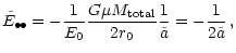 |
|
|
(19) |
 being dimensionless and
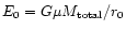 the normalization constant. The energy loss of the
binary due to gravitational radiation is (Misner et al. 1973)
the normalization constant. The energy loss of the
binary due to gravitational radiation is (Misner et al. 1973)
Forming the time derivative of Eq. (19) and with the
help of Eq. (20) the shrinking rate of the binary
results in
For convenience we introduced the dimensionless "shrinking time''
 in the last step. Multiplied with t0 this reference
time scales as
in the last step. Multiplied with t0 this reference
time scales as
 |
|
|
(22) |
Integrating Eq. (21) from
,
when the distance is
 ,
to
yields
,
to
yields
 |
|
|
(23) |
We define
 as the distance of the transition
where emission of gravitational radiation becomes more effective than
ejection of stars in extracting angular momentum from the binary.
If we now assume that the integration of the shrinking rate
(21) starts when the BHs happen
to be just this distance apart (
as the distance of the transition
where emission of gravitational radiation becomes more effective than
ejection of stars in extracting angular momentum from the binary.
If we now assume that the integration of the shrinking rate
(21) starts when the BHs happen
to be just this distance apart (
 ),
we get
),
we get
 |
|
|
(24) |
In this expression
 |
|
|
(25) |
is the time the black holes
still need to merge completely once gravitational radiation starts at
to govern the merging process.
![\begin{figure}
\par\includegraphics[width=8.8cm,clip]{fig8.eps}\end{figure}](/articles/aa/full/2001/37/aah2731/Timg239.gif) |
Figure 8:
The shrinking rates due to ejection of stars (solid line)
and emission of gravitational radiation (dashed line) are shown to
have very different slopes. Therefore the region of the transition is
quite narrow. The separation  is normalized to
.
is normalized to
. |
| Open with DEXTER |
If
in Eq. (23) is equal to 1,
i.e. the separation where we started the simulation and where the BHs are
apart from each other, the time needed to reduce
by some large fraction because of emission of gravitational
radiation only is of order of
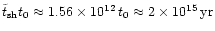 .
Thus in the
beginning, at distances as large as
,
the
hardening of the binary caused by emission of gravitational radiation is
completely negligible and proceeds on time-scales orders of magnitudes
higher
than shrinking due to ejection of stars. To compare these two
rates of hardening we have to rewrite Eq. (18) in its
dependence on distance
instead of
.
Unfortunately, because of
its complicated form, we can not build the inverse function of
.
However, to proceed we first have to further
simplify our fit function. This is done by resetting the parameter
.
Thus in the
beginning, at distances as large as
,
the
hardening of the binary caused by emission of gravitational radiation is
completely negligible and proceeds on time-scales orders of magnitudes
higher
than shrinking due to ejection of stars. To compare these two
rates of hardening we have to rewrite Eq. (18) in its
dependence on distance
instead of
.
Unfortunately, because of
its complicated form, we can not build the inverse function of
.
However, to proceed we first have to further
simplify our fit function. This is done by resetting the parameter
 to zero, so that the cut-off funtion in
Eq. (9) vanishes and we are left with
a pure power law only. In order not to have too large differences
between this fit and the data for small times and to take account of
the initial increase we shift the parameter
from
20 to 50. Hence the system function (10) becomes
to zero, so that the cut-off funtion in
Eq. (9) vanishes and we are left with
a pure power law only. In order not to have too large differences
between this fit and the data for small times and to take account of
the initial increase we shift the parameter
from
20 to 50. Hence the system function (10) becomes
 |
|
|
(26) |
To maintain the number of ejected stars needed for a final
merger of the black holes we recalculate the parameter k using
Eq. (11). Thus
 and therefore we get
 .
Since we are just interested in an estimate
of the timescales of the merger, these parameters still provide a
sufficiently good fit to the data as can be
seen in Fig. 7, where the power law is shown
as dotted line an denoted as "fit 2''. Now the distance as function of time,
.
Since we are just interested in an estimate
of the timescales of the merger, these parameters still provide a
sufficiently good fit to the data as can be
seen in Fig. 7, where the power law is shown
as dotted line an denoted as "fit 2''. Now the distance as function of time,
 ,
can be solved for .
With
,
can be solved for .
With
 the shrinking-rate
 is constant, as is found by Milosavljevic & Merritt (2001) in N-body
calculations. Substituting the time as function of the separation
together with Eq. (26) in the the shrinking rate due
to star ejection (18) yields
is constant, as is found by Milosavljevic & Merritt (2001) in N-body
calculations. Substituting the time as function of the separation
together with Eq. (26) in the the shrinking rate due
to star ejection (18) yields
 |
|
|
(27) |
Equating this expression with the hardening rate caused by emission of
gravitational waves (21) we
can solve for the distance of the transition
where gravitational radiation takes over the process of shrinking,
![$\displaystyle \tilde{a} _{\rm {tr}} = \left[\frac{1}{2(\alpha - 1)}
\left(\frac...
...{\rm {d}}}{\tilde{t} _{\rm {sh}}}
\right]^{\frac{2(\alpha-1)}{8\alpha -7}}\cdot$](/articles/aa/full/2001/37/aah2731/img249.gif) |
|
|
(28) |
The merging for
 is dominated by the
ejection of
stars. Since both shrinking rates have very different slopes (see
Fig. 8)
does not depend
sensitively on the
parameters we chose for the fit and the transition occurs quite
suddenly over a small range in .
Substituting
to
we can
solve it for the time
is dominated by the
ejection of
stars. Since both shrinking rates have very different slopes (see
Fig. 8)
does not depend
sensitively on the
parameters we chose for the fit and the transition occurs quite
suddenly over a small range in .
Substituting
to
we can
solve it for the time
 needed till the distance has
shrunk from its initial value
to
due to ejection of stars. For the
parameters we used,
and
needed till the distance has
shrunk from its initial value
to
due to ejection of stars. For the
parameters we used,
and
 ,
we
finally obtain for q=10
,
we
finally obtain for q=10
Hence after about
the distance of the two
black holes has shrunk to
 of its initial value
.
Merritt (2000) obtained for
about 1/100 of the distance where the binary
becomes hard, which translates in physical units to about
of its initial value
.
Merritt (2000) obtained for
about 1/100 of the distance where the binary
becomes hard, which translates in physical units to about
 according to Milosavljevic & Merritt (2001). This is in good agreement with the
distance of transition for the mass-ratio q=1, see
Table 1.
according to Milosavljevic & Merritt (2001). This is in good agreement with the
distance of transition for the mass-ratio q=1, see
Table 1.
Only the fraction
 of the initial angular momentum of the
binary is left at this distance. With
for the powerlaw
index the relation between the distance and time of the transition is
of the initial angular momentum of the
binary is left at this distance. With
for the powerlaw
index the relation between the distance and time of the transition is
 ,
and
Eq. (28) simplifies to
,
and
Eq. (28) simplifies to
Thus the ratio of the time ranges when star ejection and emission of
gravitational waves dominate the hardening is independent of the
massratio:
 |
|
|
(30) |
For the time when gravitational radiation dominates we then have
 |
|
|
(31) |
showing that the merging process is dominated most of the time by
ejection of stars.
Quinlan (1996) obtains for the timescales needed for
merging once the binary has become hard (
 ), about
 .
This is very
similar to our result, which is supposed to be a lower limit since in
the simulation the shrinking of the distance between the black holes has
not been taken into account.
This time-scale on which the BHs merge is of the same order as the
one we obtained for the torus to emerge, see
Fig. 2. Thus, if a binary with a mass-ratio 10merges due to ejection of stars from a surrounding cluster, a
torus-shaped distribution forms on a similar time-scale.
.
This is very
similar to our result, which is supposed to be a lower limit since in
the simulation the shrinking of the distance between the black holes has
not been taken into account.
This time-scale on which the BHs merge is of the same order as the
one we obtained for the torus to emerge, see
Fig. 2. Thus, if a binary with a mass-ratio 10merges due to ejection of stars from a surrounding cluster, a
torus-shaped distribution forms on a similar time-scale.
The energy of the binary scales with its separation as
 .
If the distances of the stars in the cluster
are increased or decreased by the same factor
.
If the distances of the stars in the cluster
are increased or decreased by the same factor  as the
binary's separation, the energy of a star also scales with this
factor to the power of -1, i.e.
and
as the
binary's separation, the energy of a star also scales with this
factor to the power of -1, i.e.
and
 .
Thus the basic
results will be unchanged as long as the binary remains "hard'', but
the time-scales of the merging due to ejection of stars scale as
.
Thus the basic
results will be unchanged as long as the binary remains "hard'', but
the time-scales of the merging due to ejection of stars scale as
 .
.
The final merger of two supermassive BHs should lead to one of
the most energetic events in the universe. As a result of such a
merger, the spin and its direction are expected to change
(Wilson & Colbert 1995). Consequently also the direction of the jet, which is
aligned with the BH's spin, will jump into the new direction of the
spin of the merged BH. This is a possible explanation for the observed
X-shaped radio galaxies. This class of objects exhibits four jets, one
pair of which shows "young'' synchrotron emission and the other one
"old'' emission, such as seen in B2 0828+23 (Parma et al. 1985; Rottmann et al. 1998).
The spectral aging of the secondary lobes in this object suggests that
a merger has happened about
 ago
(priv. communication with H. Rottmann). This timescale is very close
to the one we have found here for the merger of two supermassive BHs
and thus supports the idea of mergers inducing a jump of the jet.
ago
(priv. communication with H. Rottmann). This timescale is very close
to the one we have found here for the merger of two supermassive BHs
and thus supports the idea of mergers inducing a jump of the jet.
As we have shown in Sect. 3.1,
both populations, the ejected and bound stars, can be clearly
distinguished by their angular momentum or their pericenter.
To learn more about their angle distribution is the task of
this section. For this purpose we introduce some angles, as is
illustrated in Fig. 9.
We define
 as the angle between
the positive z-axis (the rotation axis
as the angle between
the positive z-axis (the rotation axis
 )
and
the angular momentum
)
and
the angular momentum
 of a
star. The angle between
and the negative
z-axis is denoted by
of a
star. The angle between
and the negative
z-axis is denoted by
 ,
so that
,
so that
 .
To the angle between the plane in which the star
rotates and the equatorial plane we refer as
.
To the angle between the plane in which the star
rotates and the equatorial plane we refer as
 .
.
![\begin{figure}
\par\resizebox{85mm}{!}{\includegraphics[clip]{H2731_14.eps}} %
\end{figure}](/articles/aa/full/2001/37/aah2731/Timg275.gif) |
Figure 9:
This sketch illustrates the meaning of the different
angles. The equatorial plane is defined by the black holes rotating around
each other, with the angular frequency vector
pointing along the z-axis. M1 is displayed a little off-center
since the coordinate system is centered in the center of mass
frame. Tilted to this plane with an angle
is the orbital plane of a star, whose angular
momentum
encloses the angles
with
(the positive z-axis) and
with the negative z-axis. The line from the center to the current
position of the star has the angle
 with
.
with
. |
| Open with DEXTER |
The angle which is enclosed by the line connecting the origin with the
current position of the star and the z-axis is denoted by
.
The mean and the dispersion of this angle
are very similar at
for all three populations (EP, BP, TP),
namely
 and
and
 .
These are
just the values we expect for a spherically symmetric distribution, as
the total population at
.
Thus both populations, EP and
BP, are also spherically symmetric distributed in the beginning and
none of them shows any preferences as to certain polar angles.
However, from Table 1 we see that the mean angular momentum
of the ejected stars increased by just a factor of 1.1,
while
is by more than a factor 4.5 bigger at
the end of the simulation. Thus we expect the geometry of
the distribution of the ejected population to be flattened and not
spherically symmetric at the end of the simulation.
.
These are
just the values we expect for a spherically symmetric distribution, as
the total population at
.
Thus both populations, EP and
BP, are also spherically symmetric distributed in the beginning and
none of them shows any preferences as to certain polar angles.
However, from Table 1 we see that the mean angular momentum
of the ejected stars increased by just a factor of 1.1,
while
is by more than a factor 4.5 bigger at
the end of the simulation. Thus we expect the geometry of
the distribution of the ejected population to be flattened and not
spherically symmetric at the end of the simulation.
In Fig. 10 we plotted the density of the stars in
dependence of
the cosine of
.
As stated above we see within the
fluctuation of the data a uniform
distribution for
(dashed line), according to a spherical
symmetry. But after the stars have been ejected the density has a
maximum at
 (solid line). Thus they
are concentrated towards the equatorial plane of the binary.
The same conclusion is drawn from Fig. 11.
It displays the density as a function
of the orientation of the orbital angular momentum of the stars,
(solid line). Thus they
are concentrated towards the equatorial plane of the binary.
The same conclusion is drawn from Fig. 11.
It displays the density as a function
of the orientation of the orbital angular momentum of the stars,
 .
At
(dashed line) the density is almost constant in
.
At
(dashed line) the density is almost constant in
 ,
thus there
is no special orientation prefered for the orbital plane of the
stars. The density is slightly increasing with
,
showing that the ejected stars initially are weakly corotating on
average.
,
thus there
is no special orientation prefered for the orbital plane of the
stars. The density is slightly increasing with
,
showing that the ejected stars initially are weakly corotating on
average.
![\begin{figure}
\par\includegraphics[width=85mm]{h2731f10.eps}\end{figure}](/articles/aa/full/2001/37/aah2731/Timg282.gif) |
Figure 10:
The density of the ejected stars at
(spherically symmetric distributed) and after
their ejection (
 )
as function of
their polar angle is displayed.
After being ejected the cluster is more concentrated to the
equatorial plane )
as function of
their polar angle is displayed.
After being ejected the cluster is more concentrated to the
equatorial plane
 . . |
| Open with DEXTER |
After the ejection this curve is steeply increasing, with
only few stars having
 (counter-rotating) and the
distribution having the maximum at
(counter-rotating) and the
distribution having the maximum at
 .
This means that the angular
momentum from most stars points along the rotation axis and thus their
orbital plane is aligned with the equatorial plane. Therefore the
density of the stars has a maximum in the equatorial plane and a
minimum at the poles, as seen before in Fig. 10.
The angle
between orbital and equatorial plane
(see Fig. 9) is the same for clockwise (Lz <0)
and counter-clockwise (
.
This means that the angular
momentum from most stars points along the rotation axis and thus their
orbital plane is aligned with the equatorial plane. Therefore the
density of the stars has a maximum in the equatorial plane and a
minimum at the poles, as seen before in Fig. 10.
The angle
between orbital and equatorial plane
(see Fig. 9) is the same for clockwise (Lz <0)
and counter-clockwise (
 )
rotation and is equal to the minimum
of
and
.
Gaining now angular momentum in
the z-component leads to a decreasing angle
and
increasing
.
A formerly counter-rotating star with
)
rotation and is equal to the minimum
of
and
.
Gaining now angular momentum in
the z-component leads to a decreasing angle
and
increasing
.
A formerly counter-rotating star with
 could now cross the poles (
 )
and therefore
increase the density there. But Fig. 11 shows a
decrease in
up to
)
and therefore
increase the density there. But Fig. 11 shows a
decrease in
up to
 and an
increase
towards smaller angles. Hence the gains in
are big enough in
order to deplete the polar regions and to tilt the orbital planes
of the stars after their ejection to the equatorial plane. Moving in
its plane,
of
a star changes in the range
and an
increase
towards smaller angles. Hence the gains in
are big enough in
order to deplete the polar regions and to tilt the orbital planes
of the stars after their ejection to the equatorial plane. Moving in
its plane,
of
a star changes in the range
 ,
consequently
resulting in a maximum of the density at
(Fig. 10).
So the EP changes its symmetry from spherical to cylindrical after the
interaction with the binary.
,
consequently
resulting in a maximum of the density at
(Fig. 10).
So the EP changes its symmetry from spherical to cylindrical after the
interaction with the binary.
![\begin{figure}
\par\includegraphics[width=8.8cm,clip]{fig11.eps}\end{figure}](/articles/aa/full/2001/37/aah2731/Timg290.gif) |
Figure 11:
The orientation of the angular momenta of the EP at
and after the ejection at
is
displayed. They show a strong concentration towards large positive
values, so that the orbital plane is close to the equatorial plane. |
| Open with DEXTER |
The stars which gain the most energy also gain the most angular
momentum (see Eq. (B.4)).
In Fig. 12 we plot the energy versus
after the ejection of stars. The
figure shows a
strong correlation between the energy and
 ,
confirming the
prediction of Eq. (B.4): the orbital planes of the
stars with the highest (kinetic) energies are more concentrated
towards the equatorial plane of the binary. A similar correlation is
found when the eccentricity
,
confirming the
prediction of Eq. (B.4): the orbital planes of the
stars with the highest (kinetic) energies are more concentrated
towards the equatorial plane of the binary. A similar correlation is
found when the eccentricity
 is plotted
versus the orientation of the orbits, showing that the most eccentric
trajectories (
is plotted
versus the orientation of the orbits, showing that the most eccentric
trajectories (
 )
are most
aligned with the plane in which the black holes rotate.
)
are most
aligned with the plane in which the black holes rotate.
The strong changes in
and  of the ejected stars
compared to the
almost constant values for the BP show that the BHB is
mainly influenced by the ejected stars. Provided that initially there
are enough stars, the EP can extract sufficient angular momentum
to allow the black holes to merge, as shown in Sect. 3.2.
of the ejected stars
compared to the
almost constant values for the BP show that the BHB is
mainly influenced by the ejected stars. Provided that initially there
are enough stars, the EP can extract sufficient angular momentum
to allow the black holes to merge, as shown in Sect. 3.2.
Finally we want to give in this section a crude estimate of the
stability of the remaining torus-like distribution of the bound stars,
once the BHs have merged. In a first approximation we can use the
formulae from Sect. 2.1 for collisionless systems.
With the following values,
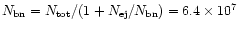 ,
,
 ,
,
 and the velocity set to the Keplerian in
a distance of
and the velocity set to the Keplerian in
a distance of
 ,
,
 ,
we obtain for the
ralaxation time
,
we obtain for the
ralaxation time
In order to get a more precise time-scale we can
make use of the diffusion coefficients D, which are a measure for the
rate at which stars diffuse through phase space as a result of
encounters, see Binney & Tremaine (1987). In the local approximation all encounters
are assumed to be local, i.e. the impact parameter b is assumed to
be much less than the system size R. Employing now the
Fokker-Planck approximation and assuming a spherical symmetry with a
Maxwellian velocity distribution Binney & Tremaine (1987) obtain for the
relaxation time, defined as
 ,
,
where
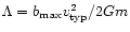 .
Here
.
Here
 is
the typical velocity of stars of the system and set to the keplerian
velocity in
distance,
is
the typical velocity of stars of the system and set to the keplerian
velocity in
distance,
 .
.
 is the maximum impact parameter and assumed to be
since
here the index of the density powerlaw changes from 2 to 4 and the
density drops quickly with increasing radius
(Fig. 1). For a mean density of
is the maximum impact parameter and assumed to be
since
here the index of the density powerlaw changes from 2 to 4 and the
density drops quickly with increasing radius
(Fig. 1). For a mean density of
 around the maximum value of
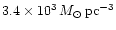 at
at
 and
and
 we
then obtain
we
then obtain
![\begin{figure}
\par\includegraphics[width=8.8cm,clip]{fig12.eps}\end{figure}](/articles/aa/full/2001/37/aah2731/Timg312.gif) |
Figure 12:
The energy at
of the EP is plotted
versus the orientation of the angular momentum. The more
energetic the stars are, the more they are concentrated to the
equatorial plane. |
| Open with DEXTER |
This time scale can now be compared to the time
 which a
star needs to spiral from the outer edge to the inner edge of the
torus due to dynamical friction. In fact, the diffusion coefficient is
identical to the deceleration of a test star owing to dynamical friction
by the surrounding field stars (Binney & Tremaine 1987),
which a
star needs to spiral from the outer edge to the inner edge of the
torus due to dynamical friction. In fact, the diffusion coefficient is
identical to the deceleration of a test star owing to dynamical friction
by the surrounding field stars (Binney & Tremaine 1987),
Again the velocity is assumed to be distributed according to a
Maxwellian and
 .
The total number density of
the stars, with each having the mass m, is denoted by n, and
.
The total number density of
the stars, with each having the mass m, is denoted by n, and  is the error-function. The decelerating force is acting tangentially and
thus causes the test star, also of mass m, to lose angular momentum
per unit mass L at a rate
is the error-function. The decelerating force is acting tangentially and
thus causes the test star, also of mass m, to lose angular momentum
per unit mass L at a rate
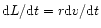 .
Following
Binney & Tremaine (1987) the star continues to orbit at the circular speed
.
Following
Binney & Tremaine (1987) the star continues to orbit at the circular speed
 as it spirals to the center and its angular momentum per unit
mass at radius r is at all times
as it spirals to the center and its angular momentum per unit
mass at radius r is at all times
 .
Equating the
time derivative with the loss rate of L due to dynamical friction
given above yields
.
Equating the
time derivative with the loss rate of L due to dynamical friction
given above yields
 .
Integrating this equation
from a radius
,
where the star starts to spiral inwards,
to the inner edge at
and solving for the time yields
.
Integrating this equation
from a radius
,
where the star starts to spiral inwards,
to the inner edge at
and solving for the time yields
The number density
 is approximated by the function
which actually is a powerlaw with index -2 in the range
 and index -4 for
 ,
while it vanishes for
,
while it vanishes for
 .
.
We chose for the
parameters
 ,
,
 and
and
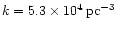 so
that the volume integration from
so
that the volume integration from
 to infinity gives the right
number of bound stars. Substituted in the expression for
and using for ,
to infinity gives the right
number of bound stars. Substituted in the expression for
and using for ,
 and
the same
values as above we obtain for the time a star needs to spiral from
distance to the inner edge of the torus at
and
the same
values as above we obtain for the time a star needs to spiral from
distance to the inner edge of the torus at
which is in good agreement with
 above. Thus we can
conclude that the torus-like structure is stable.
above. Thus we can
conclude that the torus-like structure is stable.
![\begin{figure}
\par\includegraphics[width=8.8cm,clip]{fig13.eps}\end{figure}](/articles/aa/full/2001/37/aah2731/Timg335.gif) |
Figure 13:
At the end of the simulation the more stars are ejected the bigger
M2 is. While for q=1 there is almost no cusp left in the center,
the region close to the orbit of M2 at
is not much
depleted for q=100. In the range
all density distributions follow the initial powerlaw with index
-2 while at bigger distances
 independent of q. The initial distribution is for all mass-ratios
the same and represented by the solid line. independent of q. The initial distribution is for all mass-ratios
the same and represented by the solid line. |
| Open with DEXTER |
Finally we will discuss the influence of the mass-ratio of the
black holes on the ejected and bound star populations.
In altering the mass-ratio
q = M1/M2we always keep the mass of the primary black hole fixed to
.
For the mass of the secondary we chose
M2 = 108 and
106 solar masses corresponding to the ratios q=1, 100respectively. Hence also the total mass of the binary
 is changed.
As M2 increases and q decreases the sphere of influence of
the secondary BH expands and consequently the inner regions become
more unstable. Thus a bigger fraction of stars is ejected and the
density cusp bound to the primary BH only becomes less dense, being made
up by  and
and  for q=1 and 100 respectively.
Between
for q=1 and 100 respectively.
Between
 and
and
 the
density is not much affected
by variations in q and always follows a powerlaw with
index -2 (see Fig. 13). In the heated region
(
the
density is not much affected
by variations in q and always follows a powerlaw with
index -2 (see Fig. 13). In the heated region
(
 )
too the
density does not depend on the mass ratio and the relation
holds for all q.
Due to the enhanced instability of the central region for a more
massive secondary black hole the bound stars have to be more
tangentially anisotropic in order to diminish the eccentricity of their
orbits and not to come too close to the binary. This causes the inner
edge of the torus at
)
too the
density does not depend on the mass ratio and the relation
holds for all q.
Due to the enhanced instability of the central region for a more
massive secondary black hole the bound stars have to be more
tangentially anisotropic in order to diminish the eccentricity of their
orbits and not to come too close to the binary. This causes the inner
edge of the torus at
 to be much sharper defined and thus
the maximum of the density at
to be much sharper defined and thus
the maximum of the density at
 to be
much more pronounced for
q=1, while it is almost smeared out for q=100(Fig. 13).
This is clearly visible in Fig. 14, where the density
distribution is displayed at
t=107.58 and
to be
much more pronounced for
q=1, while it is almost smeared out for q=100(Fig. 13).
This is clearly visible in Fig. 14, where the density
distribution is displayed at
t=107.58 and
 and corresponds within a factor of a few to the lower limits of the
merging times
t=106.89 and
and corresponds within a factor of a few to the lower limits of the
merging times
t=106.89 and
 of the
BHs for q=1 and 100 respectively. In fact, the bottom row for
q=100 shows no torus,
but the density is diminished around the orbit of M2 and weakly
indicates the formation of a shell-like distribution. This is
confirmed if we let the simulation continue till
,
about 10 times longer. Then the density distribution is
comparable to that of q=10 after
of the
BHs for q=1 and 100 respectively. In fact, the bottom row for
q=100 shows no torus,
but the density is diminished around the orbit of M2 and weakly
indicates the formation of a shell-like distribution. This is
confirmed if we let the simulation continue till
,
about 10 times longer. Then the density distribution is
comparable to that of q=10 after
 (2nd row in
Fig. 2).
(2nd row in
Fig. 2).
![\begin{figure}
\par\mbox{\includegraphics[width=84.75mm]{H2731_19.eps}\hspace{10...
...21.eps}\hspace{8.3mm}
\includegraphics[width=86mm]{H2731_22.eps} }
\end{figure}](/articles/aa/full/2001/37/aah2731/Timg347.gif) |
Figure 14:
Same as Fig. 2 for the final density distributions of
the mass-ratios q=1 (top row) and 100 (bottom row). For q=1there is no central cusp left and a pronounced torus with
sharp defined edges emerges after
 .
There is no torus seen in case of q=100 after .
There is no torus seen in case of q=100 after
 ,
only close to the orbit of the secondary BH the
sensity is diminished. ,
only close to the orbit of the secondary BH the
sensity is diminished. |
| Open with DEXTER |
Thus the central stellar cluster in the potential of two merging BHs
does not evolve into a torus-like structure for a sufficiently large
mass-ratio q and rather stalls in the phase when it assumes a
shell-like structure.
On the other hand we can see that in the case of q=1 the final torus
(
 )
is much more pronounced than for
q=10, compare Figs. 2 and 14.
This
means that for sufficiently small mass-ratios q a stellar torus
forms in the late stages of a merger, while for young mergers and
mergers with a big mass-ratio a shell-like density distribution is
maintained.
For q=1 in Fig. 14 the inner edge of the torus is
more sharply defined, and there is actually no cusp left in the
center.
Consequently the bound stars must have bigger angular momenta
as M2 increases. If we compare the initial angular momentum of the
ejected stars for the mass-ratios q=1 and 100 with the ratio
q=10, it turns out that it increases with the mass of the secondary
BH (decreasing with q). The relation
)
is much more pronounced than for
q=10, compare Figs. 2 and 14.
This
means that for sufficiently small mass-ratios q a stellar torus
forms in the late stages of a merger, while for young mergers and
mergers with a big mass-ratio a shell-like density distribution is
maintained.
For q=1 in Fig. 14 the inner edge of the torus is
more sharply defined, and there is actually no cusp left in the
center.
Consequently the bound stars must have bigger angular momenta
as M2 increases. If we compare the initial angular momentum of the
ejected stars for the mass-ratios q=1 and 100 with the ratio
q=10, it turns out that it increases with the mass of the secondary
BH (decreasing with q). The relation
 also holds at the end of the simulation as well as for the EP.
Plotting the initial angular momentum versus the
radius for each star for q=1 and 100, just in the same way as for
q=10 in Fig. 4, gives a very similar separation
between the EP and BP. But with increasing q the transition
value of ,
dividing both populations, decreases from a
little more than 2 for q=1 to a value below 2 for q=100 with
always the same initial conditions. As the value of transition of
in Fig. 4 is decreasing with M2,
also the mean values of the angular momentum of both populations are
decreasing. Stars which have been ejected for small mass-ratios q``defect'' to the BP as q increases and the inner region
becomes more stable. Therefore the deviation
also holds at the end of the simulation as well as for the EP.
Plotting the initial angular momentum versus the
radius for each star for q=1 and 100, just in the same way as for
q=10 in Fig. 4, gives a very similar separation
between the EP and BP. But with increasing q the transition
value of ,
dividing both populations, decreases from a
little more than 2 for q=1 to a value below 2 for q=100 with
always the same initial conditions. As the value of transition of
in Fig. 4 is decreasing with M2,
also the mean values of the angular momentum of both populations are
decreasing. Stars which have been ejected for small mass-ratios q``defect'' to the BP as q increases and the inner region
becomes more stable. Therefore the deviation
 of the
BP increases while it is decreasing for the ejected population (see
Table 1).
of the
BP increases while it is decreasing for the ejected population (see
Table 1).
The smaller the mass-ratio is, the more angular momentum is extracted
from the binary by a single ejected star on average
(
 ,
see
Table 1). But this is not
enough to compensate for the bigger amount of angular momentum of the
binary due to the more massive secondary BH,
,
see
Table 1). But this is not
enough to compensate for the bigger amount of angular momentum of the
binary due to the more massive secondary BH,
 .
Thus the cluster has to be more massive
so that the binary can transfer its angular momentum to a larger
number of ejected stars in order to merge.
To compute the required number of stars and the time
needed to enable the merging of the black holes we proceed in the same way
as before in Sect. 3.2 for q=10.
With decreasing mass-ratio the maximum of the angular momentum
lossrate is more peaked and has a value
.
Thus the cluster has to be more massive
so that the binary can transfer its angular momentum to a larger
number of ejected stars in order to merge.
To compute the required number of stars and the time
needed to enable the merging of the black holes we proceed in the same way
as before in Sect. 3.2 for q=10.
With decreasing mass-ratio the maximum of the angular momentum
lossrate is more peaked and has a value
 times higher for q=1compared to q=10 (see Fig. 15). The maximum is
reached the sooner, the smaller q is (
times higher for q=1compared to q=10 (see Fig. 15). The maximum is
reached the sooner, the smaller q is (
 corresponding to
 and
and
 for
for
 respectively). Also the powerlaw with index
-3/2 is approximated earlier by the loss-rate for small mass-ratios
and therefore the system is relaxing faster.
respectively). Also the powerlaw with index
-3/2 is approximated earlier by the loss-rate for small mass-ratios
and therefore the system is relaxing faster.
The number of stars and the times required for the merging are
listed in Table 1. The values we computed for the case
q=100 are not as accurate as for the other mass-ratios, since the
data of the angular momentum loss-rate do not allow for a fit as good
as for q=1 and 10.
However, the values show that for a binary with a fixed
mass for the primary BH more stars in the cluster are required
for smaller mass-ratios in order to allow the black holes
to coalesce. On the other hand the binary with the smaller mass-ratio
is merging faster, provided that the cluster is sufficiently
massive. For instance if q=1, the merger is 2.4 times
faster than the one where q=10, while a factor of 3.5 times more
stars in total are required.
For a binary with smaller q the distance
,
where
gravitational radiation starts to dominate the merging process,
is bigger and thus reached after a shorter time due
to the larger mass of M2(
 and
and
 for
for
 respectively, see
Table 1).
respectively, see
Table 1).
![\begin{figure}
\includegraphics[width=8.8cm,clip]{fig15.eps}\end{figure}](/articles/aa/full/2001/37/aah2731/Timg365.gif) |
Figure 15:
The smaller the mass-ratio q is, the more peaked is the
maximum and the earlier the maximum is reached. Thus the system is
relaxing faster. For all q the loss-rates finally approximate a
powerlaw with index -3/2. For q=100 the curve is not as smooth due
to the smaller number statistics. |
| Open with DEXTER |
The ratio of the time-ranges during which the
merger is dominated by ejection of stars or the emission
gravitational radiation,
 ,
is
independent of the mass-ratio and always equal to 4,
see Eq. (30).
,
is
independent of the mass-ratio and always equal to 4,
see Eq. (30).
Assuming the average stellar mass to be that of the sun, these numbers
show that the ejected mass
 is of order of the
total mass of the binary
is of order of the
total mass of the binary
 .
While
is
decreasing more strongly with increasing q than the binary mass,
the ejected mass always exceeds that of the secondary BH.
The ratio of both masses,
.
While
is
decreasing more strongly with increasing q than the binary mass,
the ejected mass always exceeds that of the secondary BH.
The ratio of both masses,
 is increasing with
q. Therefore a primary BH with mass M1ejects more mass if it merges with N black holes of mass M1/N than
merging with another BH of mass M1. This is the same result
which has been obtained by Quinlan (1996) in scattering
experiments.
is increasing with
q. Therefore a primary BH with mass M1ejects more mass if it merges with N black holes of mass M1/N than
merging with another BH of mass M1. This is the same result
which has been obtained by Quinlan (1996) in scattering
experiments.
One basic problem in our understanding of the central activity of
galaxies is addressed in this paper: do the black holes in the center
of two merging galaxies also merge?
Based on the two assumptions that galaxies contain supermassive black holes
in their centers and that galaxies merge we simulated a stellar
cluster in the potential of a BHB. When the distance between the
black holes has shrunk to
 and ejection of stars
dominates the merging, we start our calculations. Since the simulated
time is much smaller than the relaxation time of the cluster and the
potential is dominated by the mass of the two black holes we were dealing
with the restricted three body problem. The results we obtained by
solving these equations for the stars of the cluster, initially
distributed according to the singular isothermal sphere, just give an
order of magnitude estimate since in the calculations we neglected
further shrinking of the separation of the BHs due to ejection of
stars.
and ejection of stars
dominates the merging, we start our calculations. Since the simulated
time is much smaller than the relaxation time of the cluster and the
potential is dominated by the mass of the two black holes we were dealing
with the restricted three body problem. The results we obtained by
solving these equations for the stars of the cluster, initially
distributed according to the singular isothermal sphere, just give an
order of magnitude estimate since in the calculations we neglected
further shrinking of the separation of the BHs due to ejection of
stars.
We find that the angular momentum divides the stellar cluster
into a bound and
ejected population. Stars staying bound in the potential of the BHs
are distributed in a torus-like shape. Its relaxation time exceeds
 ,
so that this structure can be regarded as
stable. It can explain lots of the features which are postulated by
the unification model for a dusty torus in AGN and will be the topic
of Paper II.
,
so that this structure can be regarded as
stable. It can explain lots of the features which are postulated by
the unification model for a dusty torus in AGN and will be the topic
of Paper II.
Stars which belong to the ejected population have low angular momentum and
are moving on highly eccentric orbits, being radially
anisotropic in velocity. The distribution of their peri- and apocenter
always allows them to come very
close to the binary. Here they gain sufficient energy in violent
interactions with the black holes to become ejected.
The ejected stars gain angular momentum in their
z-component at the expense of the binary, which can be understood in
terms of the conservation of the Jacobian Integral (
 ). Thus the binary continues to
shrink. Integrating its loss-rate
). Thus the binary continues to
shrink. Integrating its loss-rate
 allows to
calculate the number of ejected stars and the time required for the
black holes to coalesce.
allows to
calculate the number of ejected stars and the time required for the
black holes to coalesce.
Starting with
distance between the BHs,
we find that a stellar cluster with a mass of order of the binary is
required to allow the BHs to coalesce.
The merging proceeds on
timescales of order of
and will change the spin of
the central BH (Wilson & Colbert 1995). Consequently also the jet, emanating
from the center, will jump and flow along the new spin direction after
the merger is completed. This might be an explanation for the observed
X-shaped radio galaxies, where a spectral aging time of the the
secondary lobes suggests that a merger has happened
 ago (priv. comm. H. Rottmann). The agreement with
our merger timescale is in favour of this idea.
ago (priv. comm. H. Rottmann). The agreement with
our merger timescale is in favour of this idea.
Most of the time (factor 4) this merging
process is dominated by ejection of stars before emission of
gravitational radiation takes over. Thus a stellar cluster with a
total mass
comparable to that of the binary is needed to allow the black holes to
merge due to the ejection of a fraction of
 of all stars.
After the ejection the stars are strongly concentrated to the
equatorial plane of the binary, the more the higher their energy is,
and the initial spherical geometry of the EP has been transformed
into a cylindrical geometry.
of all stars.
After the ejection the stars are strongly concentrated to the
equatorial plane of the binary, the more the higher their energy is,
and the initial spherical geometry of the EP has been transformed
into a cylindrical geometry.
As the mass of the secondary black hole is increased, the central
region becomes more unstable and a bigger fraction of stars
is ejected. In order
to extract sufficient angular momentum from the binary, more stars are
required, so that the clusters mass still is of the order of magnitude of
the binary's mass. The system is relaxing faster and the distance
where gravitational radiation dominates the merging process is reached
earlier, so that the binary merges on smaller time scales
(
 and
and
 for
and 100 respectively). The
ratio
is increasing with q and therefore a primary
black hole with mass M1 ejects more mass in N minor mergers with
secondary black holes of mass M2=M1/N than in one major merger with
mass M2=M1.
for
and 100 respectively). The
ratio
is increasing with q and therefore a primary
black hole with mass M1 ejects more mass in N minor mergers with
secondary black holes of mass M2=M1/N than in one major merger with
mass M2=M1.
In major mergers the mass distribution is likely to be completely
rearranged and the resulting galaxy will probably have a rather
elliptical than spiral shape. In their overview of the structure of
nearby AGN (Malkan et al. 1998) find that Seyfert 1 nuclei reside in more
early-type host galaxies than Seyfert 2. This is in agreement with our
finding, that the more massive the secondary BH is, the more stars
from the cluster are ejected.
Thus the remaining torus-like distribution
becomes shallower and there is a higher probability to see the type 1
nucleus directly.
Combinig this with the conclusions by (Wilson & Colbert 1995), that radio loud
objects are possibly the product of major mergers, it is expected that
radio loud galaxies are more likely to host type 1 nuclei.
The key result of this paper is: provided that a black hole binary is
surrounded by a cluster of solar mass stars with
 ,
i.e. the total mass of the cluster is comparable
to that of the binary, the black holes merge on time scales of about
.
In Paper II we will demonstrate that the stellar
torus surrounding the merged binary also meets the other requirements
of the unification scheme. We will demonstrate that the stellar winds
are pushed by radiation from the central source into long tails, and that
the ensemble of many stellar wind-tails can constitute the observed
torus.
,
i.e. the total mass of the cluster is comparable
to that of the binary, the black holes merge on time scales of about
.
In Paper II we will demonstrate that the stellar
torus surrounding the merged binary also meets the other requirements
of the unification scheme. We will demonstrate that the stellar winds
are pushed by radiation from the central source into long tails, and that
the ensemble of many stellar wind-tails can constitute the observed
torus.
Acknowledgements
C. Z. wishes to thank Matt Malkan, Ski Antonucci, Graeme Smith, David
Merritt and Stefan Westerhoff for their helpful discussions and their
generous and kind hospitality. We are grateful to our referee Edward
J. M. Colbert for his helpful advice and comments.
Appendix A: Equations of the restricted three body system
In the restricted three body system two massive bodies (BHs)
are circulating around each other. A third particle
(a star), whose mass is negligible
(
 ), is moving in the time dependent gravitational
potential of the massive bodies, which reads in the dimensionless form
(Eq. (3)):
), is moving in the time dependent gravitational
potential of the massive bodies, which reads in the dimensionless form
(Eq. (3)):
 .
The star is located at
.
The star is located at
 while
while
 and
and
 denote the positions of M1 and M2 respectively.
The origin is identified with the center of mass of the two massive
bodies and their axis of rotation is aligned with the z-axis and at
t=0 with both black holes situated on the x-axis.
The equations of motion for the star are
denote the positions of M1 and M2 respectively.
The origin is identified with the center of mass of the two massive
bodies and their axis of rotation is aligned with the z-axis and at
t=0 with both black holes situated on the x-axis.
The equations of motion for the star are
 |
|
|
(A.1) |
We always assumed
(and therefore
). The separation of the black holes,
 ,
is
constant, i.e. the black holes are moving on
circular orbits with a constant radius around each other.
The numerical integration of the equations of motion is processed
faster in the
comoving frame where the BHs are stationary on the
,
is
constant, i.e. the black holes are moving on
circular orbits with a constant radius around each other.
The numerical integration of the equations of motion is processed
faster in the
comoving frame where the BHs are stationary on the
 -axis in the distances
 and
and
 from
the origin. The transformation into the comoving frame
introduces the centrifugal and the Coriolis force in (A.1):
from
the origin. The transformation into the comoving frame
introduces the centrifugal and the Coriolis force in (A.1):
where
 in dimensionless units is actually the
unit-vector in z direction,
in dimensionless units is actually the
unit-vector in z direction,  .
Written in components with the vectors
.
Written in components with the vectors
 and
and
 this
equation is transformed into a system of six coupled ordinary
differential equations of first order:
this
equation is transformed into a system of six coupled ordinary
differential equations of first order:
After being supplied with a set of initial conditions these equations
have been integrated numerically.
Appendix B: The Jacobian integral
For the restricted three body problem the energy is not conserved
because the potential is time-dependent and
consequently no integral of motion. The same holds for the angular momentum,
which is not conserved since the potential is not invariant to
rotations. But an integral of motion can still be found
if we multiply the equation of motion for a star (A.3) with
 ,
,
Because
is constant and
 does not
depend explicitly on time we can rewrite this expression in a form
showing that the quantity
does not
depend explicitly on time we can rewrite this expression in a form
showing that the quantity
 |
|
|
(B.2) |
the Jacobian Integral, is conserved (
 ). With the expressions for the
energy and the specific angular momentum
expressed in the comoving frame
). With the expressions for the
energy and the specific angular momentum
expressed in the comoving frame
and using the relation
we finally can write the Jacobian Integral in the simple form
 |
|
|
(B.3) |
Thus, in a rotating non-axisymmetric potential, neither
nor
 is conserved, but the combination
 .
Applying infinitesimal variations to Eq. (B.3), with
.
Applying infinitesimal variations to Eq. (B.3), with
 ,
leads to the expression
,
leads to the expression
 |
|
|
(B.4) |
Consequently, stars which gain energy also gain angular momentum in the
z-component.
Appendix C: The isothermal sphere
In a spherically symmetric potential there exist four isolating integrals,
the energy E and the three components of the angular momentum
 .
According to the Jeans Theorem applied to spherical
systems any non-negative function of these integrals can serve as the
distribution function of a spherical stellar system. The extension of
the Strong Jeans Theorem to spherical systems by
Lynden-Bell (1962) allows to conclude that the distribution function of
any steady state spherical system can be
expressed as function a
.
According to the Jeans Theorem applied to spherical
systems any non-negative function of these integrals can serve as the
distribution function of a spherical stellar system. The extension of
the Strong Jeans Theorem to spherical systems by
Lynden-Bell (1962) allows to conclude that the distribution function of
any steady state spherical system can be
expressed as function a
 .
If the system is spherically
symmetric in all its properties, f is independent on the direction
of
so that
f = f(E, L).
If now the potential
.
If the system is spherically
symmetric in all its properties, f is independent on the direction
of
so that
f = f(E, L).
If now the potential  is provided by the stellar system itself
and we understand f as the mass distributionfunction (i.e.
is provided by the stellar system itself
and we understand f as the mass distributionfunction (i.e.
 )
the Poisson equation
)
the Poisson equation
 |
|
|
(C.1) |
is the fundamental equation which governs spherical equilibrium
stellar systems.
In spherical symmetry this equation is
 |
|
|
(C.2) |
Following the notation of Binney & Tremaine (1987) we
define the relative potential and the relative energy by
 and
and
 .
The constant
.
The constant  is choosen in a way that f > 0 for
 and f = 0 for
 .
As
,
the
relative potential
.
As
,
the
relative potential  also satisfies the Poisson equation
 with the boundary condition
 for
for
 .
A distribution function depending on the
relative energy
.
A distribution function depending on the
relative energy
 only further simplifies the spherical model. In such
systems with
only further simplifies the spherical model. In such
systems with
 the velocity dispersion
tensor is isotropic everywhere because the velocity dispersions are
the same in all spherical components
the velocity dispersion
tensor is isotropic everywhere because the velocity dispersions are
the same in all spherical components  and .
Using
this distribution function and if we choose
in
a way that
and .
Using
this distribution function and if we choose
in
a way that
 for
for
 ,
Eq. (C.2) becomes
,
Eq. (C.2) becomes
Either we may understand this equation as a non-linear equation for
 with given distribution function
 ,
or as a
linear equation for
with given .
With the choice for the distribution function for a stellar dynamical
system
,
or as a
linear equation for
with given .
With the choice for the distribution function for a stellar dynamical
system
 |
|
|
(C.4) |
Poissons equation can be rewritten as
 |
|
|
(C.5) |
Integrating now the distribution function (C.4) over all
velocities yields the
density
 .
With the help of this
expression Eq. (C.5) becomes
.
With the help of this
expression Eq. (C.5) becomes
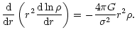 |
|
|
(C.6) |
Comparing this with the equation of
hydrostatic equilibrium for an inviscid fluid or gas
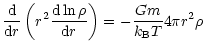 |
|
|
(C.7) |
shows that they become identical if we choose
the parameter
to be
 .
This correspondence between the gaseous and stellar-dynamical
isothermal sphere originates in the velocity distribution of both
systems. Integrating Eq. (C.4) over the
volume the distribution of velocities results in the Maxwell-Boltzmann
distribution:
.
This correspondence between the gaseous and stellar-dynamical
isothermal sphere originates in the velocity distribution of both
systems. Integrating Eq. (C.4) over the
volume the distribution of velocities results in the Maxwell-Boltzmann
distribution:
 |
|
|
(C.8) |
In order to find now a solution of Eq. (C.6) we
simply assume a powerlaw for the density (
 )
and
substitute it in Eq. (C.6) and find
)
and
substitute it in Eq. (C.6) and find
 .
Thus the two parameters must have the values b=2 and
.
Thus the two parameters must have the values b=2 and
 to fulfil this equation and we obtain for the
density
to fulfil this equation and we obtain for the
density
 |
|
|
(C.9) |
A system described by this function for the density is known as the
singular isothermal sphere, which is only true for big enough
radii because of its singularity at the center.
-
Adams, T. F. 1977, ApJS, 33, 19
In the text
NASA ADS
-
Alexander, T., & Netzer, H. 1994, MNRAS, 270, 781
In the text
NASA ADS
-
Alexander, T., & Netzer, H. 1997, MNRAS, 284, 967
In the text
NASA ADS
-
Antonucci, R. 1993, ARA&A, 31, 473
In the text
NASA ADS
-
Antonucci, R. R. J., & Miller, J. S. 1985, ApJ, 297, 621
In the text
NASA ADS
-
Barnes, J. E., & Hernquist, L. 1992, ARA&A, 30, 705
In the text
NASA ADS
-
Barvainis, R. 1987, ApJ, 320, 537
In the text
NASA ADS
-
Baugh, C. M., Cole, S., & Frenk, C. S. 1996, MNRAS, 283, 1361
In the text
NASA ADS
-
Begelman, M. C., Blandford, R. D., & Rees, M. J. 1980, nature, 287, 307
In the text
NASA ADS
-
Binney, J., & Tremaine, S. 1987, Galactic Dynamics,
Princeton Series in Astrophysics
In the text
-
Blandford, R. D. 1999, in ASP Conf. Ser. 182, Galaxy Dynamics - A Rutgers
Symposium, 87
In the text
-
Carlberg, R. G., & Couchman, H. M. P. 1989, ApJ, 340, 47
In the text
NASA ADS
-
Chandrasekhar, S. 1943, AJ, 99, 54
In the text
-
Chokshi, A., & Turner, E. L. 1992, MNRAS, 259, 421
In the text
NASA ADS
-
de Robertis, M. M., Yee, H. K. C., & Hayhoe, K. 1998, ApJ, 496, 93
In the text
NASA ADS
-
Efstathiou, A., & Rowan-Robinson, M. 1995, MNRAS, 273, 649
In the text
NASA ADS
-
Faber, S. M., Tremaine, S., Ajhar, E. A., et al. 1997, AJ, 114, 1771
In the text
NASA ADS
-
Falcke, H., & Biermann, P. L. 1995, A&A, 293, 665
In the text
NASA ADS
-
Falcke, H., Malkan, M. A., & Biermann, P. L. 1995, A&A, 298, 375
In the text
NASA ADS
-
Frenk, C. S., White, S. D. M., Davis, M., & Efstathiou, G. 1988, ApJ, 327,
507
In the text
NASA ADS
-
Fuentes-Williams, T., & Stocke, J. T. 1988, AJ, 96, 1235
In the text
NASA ADS
-
Haas, M., Müller, S. A. H., & Chini, R., et al. 2000, A&A, 354, 453
In the text
NASA ADS
-
Hemsendorf, M., Sigurdsson, S., & Spurzem, R. 2001
[astro-ph/0103410]
In the text
-
Ho, L. C., Filippenko, A. V., & Sargent, W. L. W. 1997, ApJ, 487, 591
In the text
NASA ADS
-
Innanen, K. A. 1979, AJ, 84, 960
In the text
NASA ADS
-
Innanen, K. A. 1980, AJ, 85, 81
In the text
NASA ADS
-
Kazanas, D. 1989, ApJ, 347, 74
In the text
NASA ADS
-
Kormendy, J., Byun, Y., Ajhar, E. A., et al. 1996, in IAU Symp. 171, New
Light on Galaxy Evolution, 105
In the text
-
Kormendy, J., Dressler, A., Byun ,Y. I., et al. 1994, in Dwarf Galaxies,
147
In the text
-
Krolik, J. H., & Begelman, M. C. 1988, ApJ, 329, 702
In the text
NASA ADS
-
Lawrence, A. 1991, MNRAS, 252, 586
In the text
NASA ADS
-
Lawrence, A., & Elvis, M. 1982, ApJ, 256, 410
In the text
NASA ADS
-
Lynden-Bell, D. 1962, MNRAS, 124, 1
In the text
NASA ADS
-
Macchetto, F. D. 1999, Ap&SS, 269, 269
In the text
NASA ADS
-
Madejski, G. M. 1998, in Theory of Black Hole Accretion Disks, 21
In the text
-
Magorrian, J., Tremaine, S., Richstone, D., et al. 1998, AJ, 115, 2285
In the text
NASA ADS
-
Makino, J., & Ebisuzaki, T. 1996, ApJ, 465, 527
In the text
NASA ADS
-
Malkan, M. A., Gorjian, V., & Tam, R. 1998, ApJS, 117, 25
In the text
NASA ADS
-
Merritt, D. 2000, in ASP Conf. Ser. 197, Dynamics of Galaxies: from the Early
Universe to the Present, 221
In the text
-
Mihalas, D., & Binney, J. 1981, Galactic Astronomy,
2nd Ed. (San Francisco: Freeman)
In the text
-
Mihos, J. C., & Hernquist, L. 1994, ApJ, 425, L13
In the text
NASA ADS
-
Mikkola, S., & Valtonen, M. J. 1992, MNRAS, 259, 115
In the text
NASA ADS
-
Miller, J. S., & Goodrich, R. W. 1990, ApJ, 355, 456
In the text
NASA ADS
-
Miller, J. S., Goodrich, R. W., & Mathews, W. G. 1991, ApJ, 378, 47
In the text
NASA ADS
-
Milosavljevic, M., & Merritt, D. 2001 [astro-ph/0103350]
In the text
-
Misner, C. W., Thorne, K. S., & Wheeler, J. A. 1973, Gravitation
(W. H. Freeman)
In the text
-
Miyoshi, M., Moran, J., Herrnstein, J., et al. 1995, nature, 373, 127
In the text
NASA ADS
-
Mulchaey, J. S., Myshotzky, R. F., & Weaver, K. A. 1992, ApJ, 390, L69
In the text
NASA ADS
-
Mulchaey, J. S., & Regan, M. W. 1997, ApJ, 482, L135
In the text
NASA ADS
-
Mushotzky, R. F. 1982, ApJ, 256, 92
In the text
NASA ADS
-
Nakano, T., & Makino, J. 1999, ApJ, 510, 155
In the text
NASA ADS
-
Niemeyer, M., & Biermann, P. L. 1993, A&A, 279, 393
In the text
NASA ADS
-
Noguchi, M. 1988, A&A, 203, 259
In the text
NASA ADS
-
Novikov, I. D., & Thorne, K. S. 1972, in ed. C. DeWitt, & B. S. DeWitt,
Black Holes, Les Astres Occlus, 343
In the text
-
Parma, P., Ekers, R. D., & Fanti, R. 1985, A&AS, 59, 511
In the text
NASA ADS
-
Peterson, B. M., & Wandel, A. 1999, ApJ, 521, L95
In the text
NASA ADS
-
Pier, E. A., & Krolik, J. H. 1992, ApJ, 401, 99
In the text
NASA ADS
-
Pier, E. A., & Krolik, J. H. 1993, ApJ, 418, 673
In the text
NASA ADS
-
Polnarev, A. G., & Rees, M. J. 1994, A&A, 283, 301
In the text
NASA ADS
-
Press W. H., Teukolsky, S. A., Vetterling, W. T., & Flannery, B. P. 1995,
Numerical Recipes in C, 2nd Ed.
(Cambridge University Press)
In the text
-
Protheroe, R. J., & Biermann, P. L. 1997, Astropart. Phys., 6, 293
In the text
NASA ADS
-
Quinlan, G. D. 1996, New Astron., 1, 35
In the text
NASA ADS
-
Quinlan, G. D., & Hernquist, L. 1997, New Astron., 2, 533
In the text
NASA ADS
-
Quinlan, G. D., Hernquist, L., & Sigurdsson, S. 1995, ApJ, 440, 554
In the text
NASA ADS
-
Reeves, J. N., Turner, M. J. L., Pounds, K. A., et al. 2001, A&A, 365,
L134
In the text
NASA ADS
-
Richstone, D., Ajhar, E. A., Bender, R., et al. 1998, Nature, 395, A14
In the text
NASA ADS
-
Roos, N. 1981, A&A, 104, 218
In the text
NASA ADS
-
Rottmann, H., Dennet-Thorpe, J., & Klein, U. 1998, Astronomische
Gesellschaft Meeting Abstracts, Abstracts of Contributed Talks and Posters
presented at the Annual Scientific Meeting of the Astronomische Gesellschaft
at Heidelberg, September 14-19, 1998, poster #P77, 14, 77
In the text
-
Rudge, C. M., & Raine, D. J. 2000, MNRAS, 311, 621
In the text
NASA ADS
-
Sako, M., Kahn, S. M., Behar, E., et al. 2001, A&A, 365, L168
In the text
NASA ADS
-
Sanders, D. B., Phinney, E. S., Neugebauer, G., Soifer, B. T., & Matthews,
K. 1989, ApJ, 347, 29
In the text
NASA ADS
-
Shakura, N. I., & Sunyaev, R. A. 1973, A&A, 24, 337
In the text
NASA ADS
-
Shlosman, I., Begelman, M. C., & Frank, J. 1990, Nature, 345, 679
In the text
NASA ADS
-
Taniguchi, Y. 1999, ApJ, 524, 65
In the text
NASA ADS
-
Taniguchi, Y., & Anabuki, N. 1999, ApJ, 521, L103
In the text
NASA ADS
-
Toomre, A., & Toomre, J. 1972, ApJ, 178, 623
In the text
NASA ADS
-
Tran, H. D., & Kay, L. E. 1992, in Testing the AGN Paradigm, 504
In the text
-
Urry, C. M., & Padovani, P. 1995, PASP, 107, 803
In the text
NASA ADS
-
Vecchio, A., Colpi, M., & Polnarev, A. G. 1994, ApJ, 433, 733
In the text
NASA ADS
-
Walker, I. R., Mihos, J. C., & Hernquist, L. 1996, ApJ, 460, 121
In the text
NASA ADS
-
Wang, Y., & Biermann, P. L. 1998, A&A, 334, 87
In the text
NASA ADS
-
Wills, B. J. 1999, in ASP Conf. Ser. 162, Quasars and Cosmology, 101
In the text
-
Wilson, A. S., & Colbert, E. J. M. 1995, ApJ, 438, 62
In the text
NASA ADS
-
Xu, G., & Ostriker, J. P. 1994, ApJ, 437, 184
In the text
NASA ADS
Copyright ESO 2001

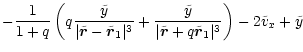
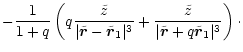
![\begin{figure}
\includegraphics[width=85mm]{h2731f1.eps}\end{figure}](/articles/aa/full/2001/37/aah2731/img107.gif)
![\begin{figure}
\par\mbox{\includegraphics[angle =-90,width=73mm]{H2731_02.eps}\h...
...s}\hspace{2.4cm}
\includegraphics[width=74.5mm]{H2731_07.eps} }
\par\end{figure}](/articles/aa/full/2001/37/aah2731/img118.gif)
![\begin{figure}
\par\includegraphics[width=8.8cm,clip]{fig3new.eps}\end{figure}](/articles/aa/full/2001/37/aah2731/img132.gif)
![\begin{figure}
\par\includegraphics[width=8.8cm,clip]{fig4new.eps}\end{figure}](/articles/aa/full/2001/37/aah2731/img133.gif)
![\begin{figure}
\par\includegraphics[width=8.8cm,clip]{fig5new.eps}\end{figure}](/articles/aa/full/2001/37/aah2731/img137.gif)
![\begin{figure}
\includegraphics[width=8.8cm,clip]{fig6.eps}\end{figure}](/articles/aa/full/2001/37/aah2731/img154.gif)
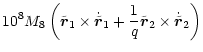
![\begin{figure}
\par\includegraphics[width=8.8cm,clip]{fig7.eps}\end{figure}](/articles/aa/full/2001/37/aah2731/img176.gif)
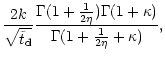
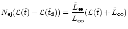
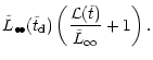
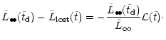
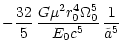
![\begin{figure}
\par\includegraphics[width=8.8cm,clip]{fig8.eps}\end{figure}](/articles/aa/full/2001/37/aah2731/img239.gif)
![\begin{eqnarray*}\tilde{a} _{\rm {tr}} = \left[\left(\frac{q+1}{q^3}\right)^{\fr...
...t} _{\rm {d}}}{\tilde{t} _{\rm {sh}}}
\right]^{\frac{1}{5}}\cdot
\end{eqnarray*}](/articles/aa/full/2001/37/aah2731/img262.gif)
![\begin{figure}
\par\resizebox{85mm}{!}{\includegraphics[clip]{H2731_14.eps}} %
\end{figure}](/articles/aa/full/2001/37/aah2731/img275.gif)
![\begin{figure}
\par\includegraphics[width=85mm]{h2731f10.eps}\end{figure}](/articles/aa/full/2001/37/aah2731/img282.gif)
![\begin{figure}
\par\includegraphics[width=8.8cm,clip]{fig11.eps}\end{figure}](/articles/aa/full/2001/37/aah2731/img290.gif)
![\begin{figure}
\par\includegraphics[width=8.8cm,clip]{fig12.eps}\end{figure}](/articles/aa/full/2001/37/aah2731/img312.gif)
![\begin{eqnarray*}\frac{{\rm d}\vec{v}}{{\rm d}t} = -\frac{8\pi \ln\Lambda G^2 m^...
...m erf}(X) -\frac{2X}{\sqrt{\pi}} {\rm e}^{-X^2}\right]\vec{v}\,.
\end{eqnarray*}](/articles/aa/full/2001/37/aah2731/img314.gif)
![\begin{eqnarray*}t _{\rm {fric}} = \frac{v_{\rm c}^3}{8\pi\ln\Lambda G^2 m^2
\le...
...^2}\right]}
\int_2^{10} \frac{1}{\tilde{r} n}{\rm d}\tilde{r}\,.
\end{eqnarray*}](/articles/aa/full/2001/37/aah2731/img321.gif)
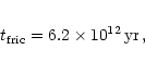
![\begin{figure}
\par\includegraphics[width=8.8cm,clip]{fig13.eps}\end{figure}](/articles/aa/full/2001/37/aah2731/img335.gif)
![\begin{figure}
\par\mbox{\includegraphics[width=84.75mm]{H2731_19.eps}\hspace{10...
...21.eps}\hspace{8.3mm}
\includegraphics[width=86mm]{H2731_22.eps} }
\end{figure}](/articles/aa/full/2001/37/aah2731/img347.gif)
![\begin{figure}
\includegraphics[width=8.8cm,clip]{fig15.eps}\end{figure}](/articles/aa/full/2001/37/aah2731/img365.gif)