A&A 376, 1135-1146 (2001)
DOI: 10.1051/0004-6361:20010996

Relaxation times calculated from angular deflections

E. Athanassoula - Ch. L. Vozikis - J. C. Lambert

Observatoire de Marseille, 2 place Le Verrier, 13248 Marseille Cedex 4, France

Received 22 February 2001 / Accepted 5 July 2001

Abstract
In this paper we measure the two-body relaxation time from the angular deflection of test particles launched in a rigid configuration of field particles. We find that centrally concentrated configurations have relaxation times that can be shorter than those of the corresponding homogeneous distributions by an order of magnitude or more. For homogeneous distributions we confirm that the relaxation time is proportional to the number of particles. On the other hand centrally concentrated configurations have a much shallower dependence, particularly for small values of the softening. The relaxation time increases with the inter-particle velocities and with softening. The latter dependence is not very strong, of the order of a factor of two when the softening is increased by an order of magnitude. Finally we show that relaxation times are the same on GRAPE-3 and GRAPE-4, dedicated computer boards with limited and high precision respectively.

Key words: celestial mechanics - stellar dynamics - galaxies: kinematics and dynamics - methods: N-body simulations

1 Introduction

Collisionless N-body simulations are heavily used to study the dynamical evolution of galaxies, or systems of galaxies, and have so far been remarkably successful in producing many interesting results. Yet proper care has to be taken to eliminate possible sources of numerical errors which could, if present, lead to erroneous results. One of the possible sources of errors stems from the fact that the number of particles in a simulation is several orders of magnitude less than the number of stars in a typical galaxy, or, in other words, that the graininess in a computer realisation is much higher than that of the galactic system it is meant to represent. This could lead to errors since a particle moving through an N-body representation of a given continuous system representing a galaxy is deflected from the orbit it would have had in the corresponding smooth continuous medium, due to two-body encounters. This effect is known as two-body relaxation and the characteristic time linked to it as two-body relaxation time (hereafter $T_{\rm relax})$.

The relaxation time will obviously increase with the number of particles in the configuration, and tend to infinity as the number of particles tends to infinity, in which limit the evolution of the system will follow the collisionless Boltzmann equation. Thus the relaxation time of simulations will be much shorter than that of galaxies, which is much longer than the age of the universe. Relaxation leads to a loss of memory of the initial conditions and an evolution of the system towards a state of higher entropy. It is thus necessary to have good estimates of the relaxation times of N-body simulations, since we can trust their results only for times considerably shorter than that.

In the early times of N-body simulations, when the number of particles used was of the order of a few hundred, the authors by necessity gave estimates of relaxation times in order to enhance the credibility of their results. Unfortunately in most cases only simple analytical estimates were used and the corresponding relaxation times were found to be comfortably, although perhaps unrealistically, high. As computers became faster, the number of particles used in simulations was increased. Authors using several tens or hundreds of thousands particles deemed it unnecessary to include such simple estimates of the relaxation times, since it was well known that the simple analytical estimates would give reassuringly high relaxation times. Nevertheless, it is not clear whether the simple analytical estimates are in all cases sufficiently near the true values. This could well be doubted since the simple analytical estimates rely on a number of approximations, which are not in all cases valid.

Since different N-body methods may lead to different relaxation rates, it is of interest to discuss relaxation times when introducing a new method. It could thus have been feared that in a tree code (Barnes & Hut 1986) the relaxation time would not be determined by the number of particles, but by the number of nodes, which would then act as "super-particles''. Since the number of nodes is always much smaller than the number of particles, this would entail considerably shorter relaxation times than direct summation with the same number of particles, and thus constitute a major disadvantage of the tree code. This fear was put to rest by Hernquist (1987) who showed that the relaxation for tree code calculations does not differ greatly from that obtained by direct summation provided the tolerance parameter is less than 1.2. Similarly Hernquist & Barnes (1990) compare relaxation rates in direct summation, tree and spherical harmonic N-body codes, while Weinberg (1996) introduces a modification of the orthogonal function potential solver that minimises relaxation.

Several methods have been used to measure two-body relaxation. Standish & Aksnes (1969), Lecar & Cruz-Conzález (1972) and Hernquist (1987) have measured the angular deflection of test particles moving in a configuration of N field particles. Although this method has the disadvantage of not including collective effects, it has the advantage that all the parameters can be changed independently of each other, and that the results are easy to interpret. Theis (1998) performed semi-analytical calculations, assuming a homogeneous medium and also ignoring cumulative effects. The most widely used approach is to monitor the energy conservation of individual particles in systems in which, had it not been for the individual encounters, the individual energies would have been conserved. This method, which includes collective effects, is well suited for testing relaxation rates introduced by different codes, but can only be used with systems in equilibrium. It has been used e.g. by Hernquist & Barnes (1990), Hernquist & Ostriker (1992), Huang et al. (1993) and Weinberg (1996). Theuns (1996) measured the diffusion coefficients as a function of the energy in a direct summation N-body simulation by studying the properties of the random walk in energy space for particles of given energy and found very good agreement with theoretically calculated diffusion coefficients. Finally a number of studies (e.g. Farouki & Salpeter 1982, 1994; Smith 1992) rely on a measurement of the mass segregation, i.e. on the fact that, due to two-body encounters, high mass particles lose energy and spiral towards the center, while light ones gain energy and move to larger radii. Thus the configuration of the high mass particles contracts, while that of the light particles expands, and from the rate at which this happens we can calculate the two-body relaxation time.

In this paper we will calculate the relaxation times in a large number of cases, using the first of the methods mentioned above, i.e. by measuring deflection angles of individual trajectories of test particles in a configuration of rigid field particles. We will cover a much larger part of the parameter space than was done so far, and we will also extend to larger number of particles. All the calculations presented in this paper were made on the Marseille GRAPE-3, GRAPE-4 and GRAPE-5 systems. The Marseille GRAPE-3 systems have been described by Athanassoula et al. (1998), while a general description of the GRAPE-4 systems and their PCI interfaces has been given by Makino et al. (1997) and Kawai et al. (1997) respectively. A description of the GRAPE-5 board can be found in Kawai et al. (2000). Opting for a GRAPE system restricts us to a single type of softening, the standard Plummer softening, but has the big advantage of allowing us to make a very large number of trials, covering well the relatively large parameter space. Theis (1998) compared the relaxation rates obtained with the standard Plummer softening to those given by a spline (Hernquist & Katz 1989) and showed that the differences between the two are only of the order of 20-40%.

This paper is organised as follows: in Sect. 2 we briefly summarise the simple analytical estimates of the relaxation time. In Sect. 3 we describe the numerical methods used in this paper and discuss the validity of their approximations. Here we also introduce the mass models which will be used throughout this paper. The values of the parameters to be used, and in particular the values of the softening, are derived and discussed in Sect. 4. In Sect. 5 we give results for the relaxation time. We specifically discuss the effect of number of particles, of the velocity and of the softening, and compare results obtained with GRAPE-3 and GRAPE-4. We also give a prediction for the relaxation time in an N-body simulation. We summarise in Sect. 6.

   
2 Simple analytical estimates of the relaxation time

The relaxation time for a single star can be defined as the time necessary for two-body encounters to change its velocity, or energy, by an amount of the same order as the initial velocity, or energy, i.e. the time in which the memory of the initial values is lost. Thus for the velocity we have

$$T_{\rm relax} = T_{\rm cross} \frac {\upsilon^2}{\Delta\upsilon_\perp^2},$$ (1)

where $T_{\rm cross}$ is the crossing time of the system. Following e.g. Binney & Tremaine (1987) we can obtain a simple order-of-magnitude estimate of the relaxation time. Let us focus on the motion of a single star assuming that it is moving on a straight line with a constant velocity v and that the remaining stars have equal mass m and are distributed uniformly in space. We first consider that the star passes a single perturber star on its rectilinear trajectory. Then the total change of its velocity component perpendicular to the trajectory is

$$\vert \delta\upsilon_\perp \vert \approx {{ 2 G m } \over {b \upsilon}},$$ (2)

where G is the gravitational constant and b is the impact parameter, i.e. the minimum distance between the two stars if there was no gravitational attraction. To find the total change, due to all the particles, we integrate over all encounters and find

$$\Delta\upsilon_\perp^2 = \int_{b_{\rm min}}^{b_{\rm max}} \de... ...upsilon^2} \ln \left(\frac {b_{\rm max}} {b_{\rm min}}\right),$$ (3)

where N is the number of stars, m is their mass, R is some characteristic radius of the system and $b_{\rm min}$ and $b_{\rm max}$ are the minimum and maximum values for the impact parameter. Using the same approximations and including a softening $\epsilon$, Huang et al. (1993) find

 

$$\Delta\upsilon_\perp^2 \frac{ 4 G^2 m^2 N}{R^2 \upsilon^2} \left[ \frac{\epsilon^2}{b_{\rm max}^2 + \epsilon^2} -\frac{\epsi... ...+\ln\frac{b_{\rm max}^2 + \epsilon^2} {b_{\rm min}^2 + \epsilon^2} \right]\cdot$$ (4)

A somewhat more elaborate derivation following the calculation of the diffusion coefficients (e.g. Chandrasekhar 1942; Spitzer & Hart 1971; Spitzer 1987; Binney & Tremaine 1987) gives

$$T_{\rm relax} = {{F \upsilon^3} \over {G^2 m \rho~\ln ( {b_{\rm max}} / {b_{\rm min}})}},$$ (5)

where $\rho$ is the density and F is a constant, roughly equal to 0.34. The quantity $\ln ( {b_{\rm max}} / {b_{\rm min}})$ is often denoted by $\ln \Lambda$ and referred to as the Coulomb logarithm.

The appropriate values of $b_{\rm min}$ and $b_{\rm max}$ in the above equations have been discussed at length in the literature. Chandrasekhar (1942) argued that $b_{\rm min}$ is the value of b for which the angular deflection of the star is equal to  ${1 \over 2} \pi$. The value of $b_{\rm max}$has been subject to considerable controversy. Chandrasekhar (1942), Kandrup (1980) and Smith (1992) have opted for a $b_{\rm max}$ of the order of the mean inter-particle distance, while others (e.g. Spitzer & Hart 1971; Farouki & Salpeter 1982; Spitzer 1987) used for $b_{\rm max}$ a characteristic radius of the system. The numerical simulations of Farouki & Salpeter (1994) argue in favour of the latter. This is further corroborated by the results of Theis (1998).

Using the estimates $b_{\rm min} = \frac {G m} {\upsilon^2}$, $b_{\rm max}=R$ and assuming virial equilibrium, so that we can use for the velocity the estimate $\upsilon^2 \approx \frac {G N m} {R}$, we find (Binney & Tremaine 1987)

$$T_{\rm relax}={{N}\over{8~\ln N}}T_{\rm cross}.$$ (6)

Similarly for the case with softening setting $b_{\rm min} \ll \epsilon$, $b_{\rm max}=R$ and estimating the velocity by assuming virial equilibrium we find

 

$$T_{\rm relax} {{{\rm\upsilon}^4 R^2}\over{G^2 M^2}}~ {{N}\over {4\left[\ln(R^2/\epsilon^2)-1\right]}}T_{\rm cross}$$ =

$${{{\rm\upsilon}^4 R^2}\over{G^2 M^2}}~ {{N}\over {8\ln(R/\epsilon)}}T_{\rm cross}$$ = (7)

$${{N}\over{8\ln(R/\epsilon)}}T_{\rm cross}.$$ =

Equation (7) differs by a factor of 2 from that of Huang et al. (1993), the reason being that our definition of the relaxation time is based on the velocities, while that of Huang et al. (1993) is based on the energies.

It is clear that, for the number of particles used in present-day simulations of collisionless systems and the appropriate values of the softening, N is considerably larger than $R/\epsilon$. Since, however, only the logarithms of these quantities enter in Eqs. (6) and (7), the differences in the estimates of the relaxation times differ, for commonly used values of N, by less than a factor of 2. Equation (7) is more appropriate, since it includes the softening. Often a coefficient g is introduced in the Coulomb logarithm, i.e. $\Lambda~=~g N$. Giersz & Heggie (1994) estimated that the most appropriate value of g is 0.11. They also compiled in their Table 2 the values given by several other authors. They are all between 0.11 and 0.4. Independent of what is chosen for the Coulomb logarithm, equations such as (6) or (7) argue that even for a moderately low number of particles, of the order of say a few thousands, the relaxation time is comfortably high, of the order of, or higher than, 40 crossing times.

   
3 Numerical methods

3.1 Method

Following Standish & Aksnes (1969), Lecar & Cruz-Conzález (1972) and Hernquist (1987) we will measure relaxation using the angular deflection suffered by a test particle moving in a configuration of N field particles fixed in space.

Let us consider a sphere of a given density profile represented by N fixed particles, which we will hereafter refer to as field particles, and let us place a test particle of zero mass at the edge of this sphere either at rest, or with a radial velocity v. In the limit of $N \rightarrow \infty$ its trajectory will be a straight line passing through the center of the sphere, which we will hereafter call the theoretical trajectory. For a finite N, however, the test particle will be deflected by a number of encounters with the field particles and thus it will cross the surface of the sphere at an angle $\Phi$ from the corresponding theoretical point. Following Standish & Aksnes (1969), or Lecar & Cruz-Conzález (1972), we can measure the relaxation time as

$$T_{\rm relax}=\frac{T_{\rm t}}{\sin^2\Phi},$$ (8)

where $T_{\rm t}$ is the crossing or transit time. Different realisations of the adopted model will of course give somewhat different relaxation times. It is thus better to use an estimate based on the average of many realisations or trajectories. Thus we have (Standish & Aksnes 1969)

$$T_{\rm relax}=\frac{<T_{\rm t}>}{< \sin^2\Phi>},$$ (9)

where the <> denote an average over all realisations and/or all trajectories.

We will repeat such calculations here, extending them to non-homogeneous density distributions, different initial velocities of the test particle and a larger range of field particle numbers N. This will allow us to discuss the effect of central concentration, of initial test particle velocities, of softening and of particle number on the relaxation time.

   
3.2 Mass distributions and computing miscelanea

To find the effect of central concentration on the relaxation time we use three different mass distributions, namely the homogeneous sphere (hereafter model H), the Plummer model (hereafter model P) and the Dehnen sphere (Dehnen 1993 - hereafter model D). For the Plummer model the density is

$$\rho (r) = \frac {3 M_{\rm T}} {4\pi a_{\rm P}^3} (1 + r^2/a_{\rm P}^2)^{-5/2}$$ (10)

and for the Dehnen one

$$\rho (r) = {{(3-\gamma) M_{\rm T}} \over {4 \pi}} {{a_{\rm D}} \over {r^{\gamma}(r+a_{\rm D})^{(4-\gamma)}}},$$ (11)

where $M_{\rm T}$ is the total mass of the sphere, $a_{\rm P}$ and $a_{\rm D}$ are the two scale-lengths, of the Plummer and Dehnen models respectively, and $\gamma$ is the concentration index of the latter. For the model P we have taken a scale-length of $a_{\rm P} = 9.2$, and for model D we have adopted $a_{\rm D}=3.1$ and $\gamma=1$. In all the examples in Sects. 5.1 to 5.4 we have truncated the mass distributions, using a cut-off radius of 20, and taken the mass within this cut-off radius to be equal to 15. For these parameters the mass inside the cut-off radius is 75% of the total. For the homogeneous sphere we have adopted a cut-off radius of 20 and a mass of 15, so as to keep as much in line as possible with the other two models. For the gravitational constant we use G=1.

These three models span a large range of central concentrations. They have the same cut-off radius, but the radius containing 1/10 of the total mass is for model D roughly one fourth of the corresponding radius for model P and roughly an order of magnitude smaller than that of model H. Similarly the radius containing half the mass for model D is roughly half of that of model P and a third of that of model H. These models will thus allow us to explore fully the effect of central concentration on the relaxation time.

We start 1000 test particles from random positions on the surface of a sphere of radius 20 and with initial radial velocities equal to $f_{\rm v}$ times their theoretical escape velocity (hereafter $v_{\rm esc}$), calculated from the model. The particles were advanced using a leap-frog scheme with a fixed time-step of $\Delta t = 2 ^ {-6} = 0.015625$. We made sure this gives a sufficient accuracy by calculating orbits without the use of GRAPE and with this time-step. This showed that the energy is conserved to 8 or 9 digits. We then repeated the exercise using a Bulirsch-Stoer scheme (Press et al. 1992) and found that the energy was conserved to 10 digits. Since an accuracy of 8 or 9 digits is ample for our work, we adopted the leap-frog integrator and the afore-mentioned time-step.

The forces between particles were calculated using one of the Marseille GRAPE-3AF systems, except for the results given in Sects. 5.4 and 5.5, where we used the Marseille GRAPE-4 system.

For each model we take 10 different field particles distributions and for each we calculate the 1000 test particles trajectories. For simplicity the test particles are the same in each of the 10 field particles distributions. For each of the test particles we calculate $T_{\rm t}$ and the deflection angle from the theoretical (straight line) orbit, $\Phi$. Then the relaxation time is calculated using Eqs. (8) and (9). The errors are obtained using the bootstrap method (Press et al. 1992). In Figs. 3 to 5 error bars are plotted only when $\sigma_{T_{\rm relax}}/T_{\rm relax} > 0.05$.

3.3 Validity of the approximations

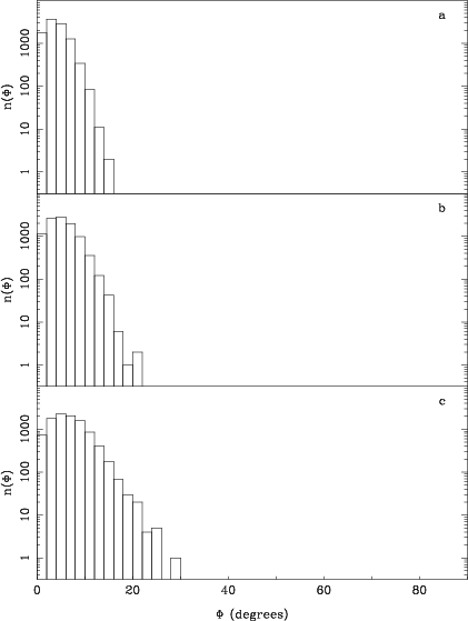	Figure 1: Distribution of the number of test particles orbits that have a given deflection angle, $n(\Phi )$, as a function of that angle for model D and $f_{\rm v}=1.5,\,\epsilon =0.01$ and N=4000 a), N=2000 b) or N=1000 c).
Open with DEXTER

Equations (8) and (9) were derived assuming small deflection angles. There could, however, be cases in which a test particle comes very near a given field particle and is very strongly deviated from its initial trajectory, so that the deflection angle is greater than 90 $\hbox{$^\circ$ }$. In that case Eqs. (8) and (9) are certainly not valid, particularly since for a deflection of 180 $\hbox{$^\circ$ }$ they will give the same result as for 0 $\hbox{$^\circ$ }$. It is not easy to treat such deflections accurately, so what we will do here is to keep track of their number and make sure that it is sufficiently small so as not to influence our results. We have thus monitored the number of orbits whose velocity component along the axis which includes the initial radial velocity changes sign. We will hereafter for brevity call such orbits looping orbits. None were found for the homogeneous sphere distribution, and very few, 3 in 10000 at the most, for the case of the Plummer sphere, and that for the smallest of the softenings used here (cf. Sect. 5.3 and Fig. 5). The largest number of looping orbits was found, as expected, for model D and the smallest softening, i.e. $\epsilon=2^{-12}$. For this case, $f_{\rm v}=1.5$ and N = 64000, we find of the order of 30 such orbits in 10000. Although this is considerably larger than the corresponding number for homogeneous and Plummer spheres, it is still low enough not to influence much our statistics, particularly if we take into account that it refers to an exceedingly small softening. For the more reasonable value $\epsilon=2^{-9}$, we find that there are no looping orbits at all. We can thus safely conclude that the number of particles with looping orbits is too low to influence our results.

We still have to make sure that the remaining orbits have sufficiently small deflection angles for Eqs. (8) and (9) to be valid. Figure 1 shows a histogram of the number of test particles orbits that have a given deflection angle, $n(\Phi )$, as a function of that angle, $\Phi$, for model D, i.e. the one that should have the largest deflection angles, with $f_{\rm v}=1.5$, $\epsilon =0.01$. The upper panel corresponds to N=4000, the middle one to N=2000 and the lower one to N=1000. Note that we have used a logarithmic scale for the ordinate, because otherwise the plot would show in all cases only a few bins near $0\hbox{$^\circ$ }$.

For N=1000 there is one particle with deviation of $28\hbox{$^\circ$ }$, one with $26\hbox{$^\circ$ }$ and two with $25\hbox{$^\circ$ }$. Furthermore only 30 trajectories, of a total of 10000, have a deflection angle larger than $20\hbox{$^\circ$ }$. The numbers are even more comforting for N=2000, where only two trajectories have a deflection angle larger than $20\hbox{$^\circ$ }$, and even more so for N=4000, where no particles reach that deflection angle. We can thus conclude that in all but very few cases the small deflection angle hypothesis leading to Eqs. (8) and (9) is valid.

   
4 Free parameters

We will calculate the values of the relaxation time as a function of three free parameters, namely the number of field particles, the initial velocity of the test particles and the softening. In this section we will discuss what the relevant ranges for these parameters are.

   
4.1 Number of particles

We will consider numbers of particles between 1000 and 64000. Indeed fewer than 1000 particles are hardly used anymore in numerical simulations, even with direct summation. For more than 64000 particles the two-body relaxation is small. Furthermore the range considered is sufficiently large for all trends to be clearly seen.

   
4.2 Initial velocity

The question for the initial velocity is more convoluted. The simple analytical approaches leading to Eqs. (6) and (7), instead of taking a spectrum of velocities for the individual encounters and then integrating over these velocities, introduce an effective or average velocity and assume that all interactions are made at this velocity. In our numerical calculations individual encounters occur at different velocities, depending on their position on the trajectory of the test particle and on the initial velocity of this particle. We can, nevertheless, introduce $v_{\rm eff}$, an average or effective velocity, in a similar way as the analytical approximation. A simple and straightforward, albeit not unique, such definition can be obtained as follows: let us assume that the test particle moves on a straight line. At each point of its trajectory we can define a thin sheet going through this point and locally perpendicular to the trajectory. It will contain all field particles which have this point as their closest approach with the test particle. Let dr be the thickness of this sheet and $\lambda {\rm d}r$ the fraction of the total mass of the field particles that is in it. Then we can define the effective velocity

$$v_{\rm eff} = 2 \int_0^R \lambda v~ {\rm d}r,$$ (12)

which of course depends on both the distribution of the field particles and the initial velocity of the test particle.

   
4.3 Softening

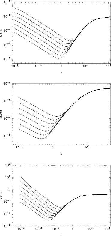Figure 2: MASE as a function of the softening $\epsilon$ for the three models described in this paper. The upper panel gives the results for model H, the middle one for model P, and the lower one for model D. In each panel from top to bottom the curves correspond to N = 1000, 2000, 4000, 8000, 16000, 32000 and 64000, where N is the number of particles in the realisation of each model. The number of realisations taken in all cases is $6 \times 10^6 / N$. The position of the minimum error along a line corresponding to a given N is marked by a $\times$, and the corresponding $\epsilon$value is the optimal softening $\epsilon _{\rm opt}$ for this number of particles.

Open with DEXTER

The third free parameter in our calculations is the softening. Merritt (1996; hereafter M96) and Athanassoula et al. (2000; hereafter AFLB) showed that, for a given mass distribution and a given number of particles N, there is a value of the softening, called optimal softening $\epsilon _{\rm opt}$, which gives the most accurate representation of the gravitational forces within the N-body representation of the mass distribution. For values of the softening smaller than $\epsilon _{\rm opt}$ the error in the force calculation is mainly due to noise, because of the graininess of the configuration. For values of the softening larger than $\epsilon _{\rm opt}$ the error is mainly due to the biasing, since the force is heavily softened and therefore far from Newtonian. Since the two-body relaxation is also a result of graininess it makes sense to consider softening values for which it is the noise and not the bias that dominates, i.e. to concentrate our calculations mainly on values of the softening which are smaller than or of the order of $\epsilon _{\rm opt}$, keeping in mind that too small values of the softening have no practical significance. The value of the optimal softening decreases with N and can be well approximated by a power law

$$\begin{eqnarray*}\epsilon_{\rm opt}=BN^{b}, \end{eqnarray*}$$

(M96). The values of B and b depend on the mass distribution under consideration, and, to a much smaller degree, on the range of N considered (AFLB). Thus denser configurations require smaller softenings for an optimum representation of the force (AFLB). For a given number of particles the homogeneous and Plummer spheres have roughly the same optimal softening, while the Dehnen sphere with $\gamma=0$ has an optimal softening 0.45 dex lower (cf. Fig. 9 of AFLB).

M96 and AFLB have calculated $\epsilon _{\rm opt}$ using the mean average square error (MASE) of the force, which measures how well the forces in an N-body representation of a given mass distribution represent the true forces in this distribution. The average square error (ASE) is defined as

$$ASE=\frac{\cal C}{N} \sum_{i=1}^{N}\vert F_i- F_{\rm true}(x_i)\vert^2,$$ (13)

where $F_{\rm true} (x_i)$ is the true force from a given mass distribution at a point x_i, F_i is the force calculated at the same position from a given N-body realisation of the mass distribution and using a given softening and method, N is the number of particles in the realisation, and the summation is carried out over all the particles. In order to get rid of the dependence on the particular configuration, which is of no physical significance, many realisations of the same smooth model must be generated and the results should be averaged over them. Thus MASE, the mean value of the ASE, is

$$MASE = \frac {\cal C} {N} <\sum_{i=1}^{N}\vert F_i- F_{\rm true}(x_i)\vert^2>$$ (14)

where <> indicates an average over many realisations. In Eqs. (13) and (14) ${\cal C}$ is a multiplicative constant, introduced to permit comparisons between different mass distributions. Since in this paper we are only interested in the values of $\epsilon _{\rm opt}$ we will simply use ${\cal C} = 1$. The MASE values were found using $6 \times 10^6 / N$ realisations and were calculated using direct summation on the Marseille GRAPE-5 systems.

Figure 2 shows values of MASE as a function of $\epsilon$ for the three models considered in Sects. 5.1 to 5.4 and seven values of N, in the range of values considered here (cf. Sect. 4.1). The general form of the curves is as expected. There is in all cases a minimum error between the region dominated by the noise (small values of the softening) and the region dominated by the bias (large values of the softening). This minimum - marked with a $\times$ in Fig. 2 - gives the value of $\epsilon _{\rm opt}$. For all three models a larger number of particles corresponds to a smaller error and a smaller value of $\epsilon _{\rm opt}$, as expected (M96, AFLB).

The more concentrated configurations give smaller values of $\epsilon _{\rm opt}$, as already discussed in AFLB. Thus for $N=64\,000$the optimum softening for model H is less than twice that of model P, while the ratio between the softenings of models P and D is more than 10.

Comparing our results to those of AFLB we can get insight on the effect of the truncation radius. For this it is best to compare our results obtained with $N = 32\,000$ with those given by AFLB for $N = 30\,000$, since these two N values are very close and we do not have to make corrections for particle number. For our model P and $N = 32\,000$ we find an optimum softening of 0.52, or, equivalently, 0.057$a_{\rm P}$, where $a_{\rm P}$ is the scale length of the Plummer sphere. This is smaller than the value of 0.063$a_{\rm P}$ found for the AFLB Plummer model and the difference is due to the different truncation radii of the two models. AFLB truncated their Plummer sphere at a radius of 38.71$a_{\rm P}$, which encloses 0.999 of the total mass of the untruncated sphere, while model P is truncated at 2.2$a_{\rm P}$, which contains only 75% of total mass. The difference in the values of $\epsilon _{\rm opt}$ is in good agreement with the discussion in Sect. 5.2 of AFLB. When the truncation radius is large, the model includes a relatively high fraction of low density regions, where the inter-particle distances are large. This is not the case if the truncation radius is much smaller, as it is here. Thus the mean inter-particle distance is larger in the former case and, as can be seen from Fig. 11 of AFLB, the corresponding optimal softening also. This predicts that the optimal softening should be smaller in models with smaller truncation radius, and it is indeed what we find here.

Our model H is the same as that of AFLB, except for the difference in the cut-off radii. Thus the values of the optimum softening are the same, after the appropriate rescaling with the cut-off radii has been applied. Our model D differs in two ways from the corresponding model of AFLB. We use here $\gamma=1$, while AFLB used $\gamma$= 0. We also truncated our model at 6.5$a_{\rm D}$, while AFLB truncated theirs at 2998$a_{\rm D}$. It is thus not possible to make any qualitative or quantitative comparisons.

   
5 Relaxation measured from angular deflections

   
5.1 The effect of the number of particles and of the density distribution

 

 

Table 1: Coefficients of linear regression in log-log scale of $T_{\rm relax}$ as a function of particle number N.

Model	$f_{\rm v}$	$\epsilon$	A1	B1	$\sigma_{A_1}$	$\sigma_{B_1}$
H			0.78	1.00	0.05	0.01
P	1.5	0.01	0.76	0.98	0.04	0.01
D			0.63	0.78	0.04	0.01
H			0.87	1.01	0.05	0.01
P	1.5	0.03	0.80	1.00	0.11	0.03
D			0.86	0.77	0.11	0.03
H			0.99	1.01	0.06	0.01
P	1.5	0.10	0.94	1.00	0.11	0.03
D			0.75	0.89	0.07	0.02
H			1.13	1.02	0.08	0.02
P	1.5	0.50	1.24	0.98	0.07	0.02
D			1.29	0.94	0.07	0.02
H			1.17	1.01	0.04	0.01
P	2.0	0.03	0.98	1.01	0.08	0.02
D			0.78	0.87	0.12	0.03
P	3.0	0.01	1.40	0.97	0.04	0.01

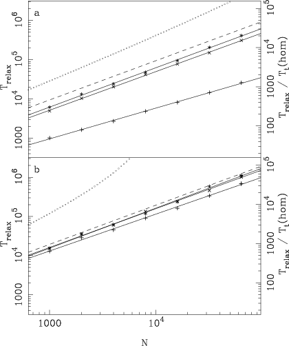Figure 3: Relaxation time as a function of the number of field particles, for $f_{\rm v}=1.5$ and three different mass models, namely model H (stars), model P ($\times$) and model D (crosses). The upper panel a) was obtained with $\epsilon =0.01$ and the lower b) with $\epsilon =0.5$. The straight solid lines are the corresponding linear least square fits. The dashed lines give the predictions of Eq. (7), when we use $b_{\rm max}=R$, while the dotted lines give the prediction of the corresponding equation obtained by using $b_{\rm max}=l$.

Open with DEXTER

Figure 3 shows the relaxation time as a function of the number of particles for the models H, P and D described in the previous section. The upper panel was obtained for $f_{\rm v}=1.5$ and $\epsilon =0.01$ and the lower one for $f_{\rm v}=1.5$ and $\epsilon =0.5$. As can be seen from Fig. 2, for the first value of the softening noise dominates over bias for all three models. For the second value noise dominates for model H, bias dominates for model D, and we are near the optimum value for model P and the high N values. The left ordinate in Fig. 3 gives the relaxation time while the right one gives the ratio of the relaxation to transit time for the homogeneous sphere and $f_{\rm v}=1.5$. The corresponding values of this ratio for the other two density distributions can be easily obtained if one takes into account that for $f_{\rm v}=1.5$ the three theoretical transit times are 20.35, 17.52 and 16.91, for the H, P and D models respectively. We fitted straight lines

$$\begin{eqnarray*}\log_{10}(T_{\rm relax}) = A_1 + B_1 \log_{10}(N) \end{eqnarray*}$$

to each model using least-square fits and plotted them with solid lines in the figure. The values of A₁ and B₁, as well as of their corresponding uncertainties $\sigma_{A_1}$ and $\sigma_{B_1}$, are given in Table 1. We have performed similar calculations for other values of the velocity and softening parameters and have included in this Table the corresponding values of A₁ and B₁, as well as their uncertainties. From Fig. 3, other similar plots for other values of the softening and of the initial velocity (not presented here), and the values given in Table 1 we can reach a number of conclusions.

The dependence of $T_{\rm relax}$ on N is reasonably well represented by a straight line in the log-log plane and that for all values of the softening and $f_{\rm v}$ we tried and for all three models. The relaxation time for model D is always smaller than that for models P and H. The difference is much more important (${\sim} 1$ dex) for the smaller value of the softening, than for the larger one ( ${\sim} 0.15$ dex). Similarly, the relaxation time for Plummer distributions is somewhat smaller (${\sim}0.1$ dex) than that of the homogeneous one for small values of the softening, while for the larger value the two relaxation times do not differ significantly.

Figure 3 and Table 1 also show a trend for the slopes of the straight lines. For the small softening the homogeneous model has a relaxation time which is roughly proportional to the number of field particles in the configuration, and that is in good agreement with Eq. (7). This is not true any more for the more centrally concentrated mass distributions, which have a value of B₁less than unity. For model P the value of B₁ is slightly less than unity, but for model D it is considerably so. Thus when we increase the number of particles in the configuration, we increase the relaxation time relatively less in more centrally concentrated configurations than in less centrally concentrated ones. In other words not only is the relaxation time smaller in the more centrally concentrated configurations, but also it takes more particles to increase it by a given amount.

These trends for the slopes of the straight lines are also present for the larger value of the softening. The differences, however, between the slopes, i.e. between the corresponding values of B₁, are much smaller. Thus for $f_{\rm v}=1.5$ and $\epsilon =0.01$ there is a difference of roughly 25% between the slopes corresponding to models H and D, while this value is reduced to roughly 8% when $\epsilon =0.5$.

Figure 3 also compares the prediction of Eq. (7) with the results of our numerical calculations for the homogeneous sphere. The agreement is fairly good, particularly for the larger softening, where the difference is of the order of 0.08 dex. It should be noted that these predictions were obtained with $b_{\rm max}=R$, the cutoff radius of the system. A yet better agreement would have been possible if one used $b_{\rm max}=fR$, where f is a constant larger than 1. Since, however, this constant is a function of the softening used and perhaps also of the value of $f_{\rm v}$, it is not very useful to determine its numerical value. The results obtained by using $b_{\rm max}=l$, where l is the mean inter-particle distance, are given by open squares. We note that they give a bad approximation of the numerical results, particularly so for a large number of particles and for the value of the softening which is nearest to optimal. For the smaller softening the approximation with $b_{\rm max}=l$ is still considerably worse than that obtained with $b_{\rm max}=R$, but the difference is smaller than in the case of the optimal softening. Whether this will be reversed for an even smaller value of the softening or not is not possible to predict from the above calculations. Nevertheless, if it did happen, it would be for a value of the softening that gave a very bad representation of the forces within model H. Thus we can conclude that, at least for collisionless simulations which have a reasonable softening, the simple analytical estimates presented in Sect. 2 give a reasonable approximation of the relaxation time if we use $b_{\rm max}=R$, but not if we use $b_{\rm max}=l$. The latter gives too high a value of the relaxation time, and is therefore falsely reassuring.

We also compared our results with theoretical estimates using $\ln\Lambda=\ln(gN)$ for the Coulomb logarithm and different values of g, as tabulated by Giersz & Heggie (1994). We find that they always fare less well than Eq. (7) with $b_{\rm max}=R$, particularly for $\epsilon =0.01$. Amongst the values tried, g= 0.11, proposed by Giersz & Heggie (1994), gave the best fit for $\epsilon =0.5$, while the value g= 0.4(Spitzer 1987) was best for $\epsilon =0.01$. The differences between the results for various values of g are nevertheless small.

To summarise this section we can say that more centrally concentrated distributions have smaller relaxation times and that the difference is more important for smaller values of the softening. This argues that the relaxation time is more influenced by the maximum rather than by the average density.

   
5.2 The effect of velocity

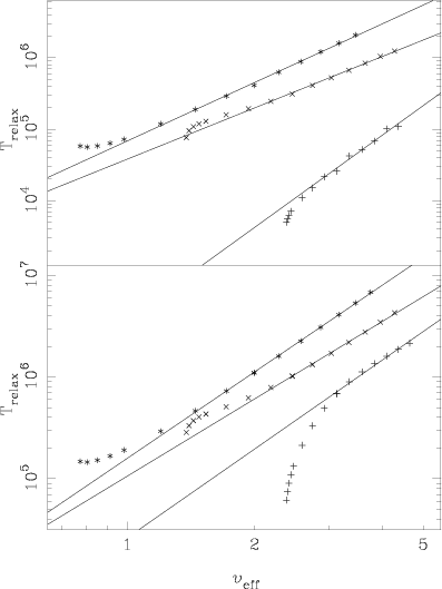	Figure 4: Relaxation time as a function of the effective velocity of the test particles, for $N=64\,000$ and three different mass models, namely model H (stars), model P ($\times$) and model D (crosses). The straight lines are the corresponding linear least square fits. The upper panel corresponds to $\epsilon =0.01$ and the lower one to $\epsilon =0.5$.
Open with DEXTER

  

 

Table 2: Coefficients of linear regression in log-log scale of $T_{\rm relax}$ as a function of $v_{\rm eff}$.

Model	$\epsilon$	A2	B2	$\sigma_{A_2}$	$\sigma_{B_2}$
H		4.84	2.72	0.02	0.04
P	0.01	4.58	2.39	0.02	0.04
D		2.33	4.28	0.20	0.35
H		5.20	2.83	0.01	0.02
P	0.5	5.02	2.53	0.02	0.04
D		4.42	2.90	0.06	0.11

In order to test the effect of velocity on the relaxation time we have launched test particles with different initial velocities.

Figure 4 shows the relaxation time as a function of the effective velocity of the particles, defined in Sect. 4, for the three density distributions under consideration. The calculations have been made with 64000 field particles and a softening of 0.01 for the upper panel and 0.5 for the lower one. The dependence is linear in the log-log plane for large values of the effective velocity and deviates strongly from it for small values. We thus fitted a straight line in the log-log plane to the higher velocities estimating for each of the mass models separately the number of points that could be reasonably fitted by a straight line. We give the constants of the regression

$$\begin{eqnarray*}\log_{10}(T_{\rm relax}) = A_2 + B_2 \log_{10} ({v_{\rm eff}}), \end{eqnarray*}$$

together with the corresponding error estimates, in Table 2.

In all cases the relaxation time increases with the initial velocity of the particles. In order to compare this with the analytical predictions of Sect. 2 we note that the deviation of a particle from its trajectory due to an encounter should be smaller for larger impact velocities (cf. Eq. (2)), while larger impact velocities imply smaller crossing times. Thus from Eqs. (6) and (7) we note that $T_{\rm relax}$ should be proportional to the third power of the velocity, i.e. that the coefficient B₂ in Table 2 should be roughly equal to 3. We note that in the homogeneous case, which should be nearer to the analytical result, there is a difference of less than 10%, presumably due to the fact that the approximations of the analytical approach are too harsh. The differences with the results of models P and D are on average larger, but strictly speaking, Eqs. (6) and (7) do not apply to them.

   
5.3 The effect of softening

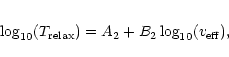
	Figure 5: Relaxation time as a function of the softening, for $N=64\,000$, $f_{\rm v}=1.5$ and three different mass models, namely model H (stars), model P ($\times$) and model D (crosses).
Open with DEXTER

Figure 5 shows the relaxation time $T_{\rm relax}$ as a function of the softening $\epsilon$ for the case of $N=64\,000$ and $f_{\rm v}=1.5$. We note that the relaxation time increases with softening as expected. There is no simple linear dependence between the two plotted quantities. In fact the relaxation time increases much faster with $\log\epsilon$ for large values of the softening than for small ones. The point at which this change of slope occurs is roughly the same for models H and P, and much smaller for model D. In fact in all cases it is roughly at the position of the corresponding optimal softening, which is roughly the same for models H and P and considerably smaller for model D (cf. Sect. 4.3). Thus the change of slope must correspond to a change between a noise dominated regime and a bias dominated one.

In the noise dominated regime the sequence between the three models is the same as in previous cases. Namely it is model H that has the largest relaxation time, followed very closely by model P, and less closely by model D. It is interesting to note that for high values of the softening the three curves intersect. Such values, however, are too dominated by bias to be relevant to N-body simulations.

Figure 5 shows the only examples in this paper in which the error bars are large enough to be plotted, i.e. for which $\sigma_{T_{\rm relax}}/T_{\rm relax} > 0.05$. These occur for the smallest values of the softening, used here more for reasons of completeness than for their practical significance.

   
5.4 GRAPE-3 results compared to GRAPE-4 results

All results presented so far were made on one of the Marseille GRAPE-3 systems (Athanassoula et al. 1998). Such systems, however, are known to have limited accuracy, since they use 14 bits for the masses, 20 bits for the positions and 56 bits for the forces. One could thus worry whether this would introduce any extra graininess, which in turn would decrease the relaxation time.

 

 

Table 3: Relaxation time $T_{\rm relax}$ of model D with $f_{\rm v}=1.5$ and $\epsilon =0.01$, obtained by the GRAPE-3 (G3) and GRAPE-4 (G4) machines.

N	G3	G4	$\Vert$G3-G4$\Vert$/G4
1000	1040	1007	0.0328
2000	1626	1633	0.0043
4000	2698	2707	0.0033
8000	4834	4845	0.0023
16000	8143	8123	0.0025
32000	14490	14548	0.0040
64000	25858	25860	0.0001

In order to test this we repeated on GRAPE-4, which is a high accuracy machine, some of the calculations made also with GRAPE-3. For this purpose, we ran 7 configurations of model D with $f_{\rm v}=1.5$, $\epsilon =0.01$ and different number of field particles. The calculated relaxation time, $T_{\rm relax}$, obtained by the GRAPE-3 and GRAPE-4 runs, together with their differences, are shown in Table 3. As we can see the results have, in all but one case, a difference less than 0.5%. Only in the case of N=1000 does the difference rise to 3%, but as we mentioned before, this very low number of particles is hardly used nowadays, even in direct summation simulations on a general purpose computer.

   
5.5 Predicting the value of T $\mathsf{_{relax}}$ for an N-body simulation

In the standard version of the angular deflection method we have used so far all the test particles start from the same radius with the same initial velocity. On the other hand in any N-body realisation of a given model the particles have different apocenters. It is thus necessary to extend this method somewhat in order to obtain an estimate of how long a given N-body simulation will remain unaffected by two-body relaxation. Let us consider a simple model consisting of a Plummer sphere of total mass 20 and scale length 9.2, truncated at a radius equal to 30.125, i.e. at a radius containing roughly 7/8 of the total mass. As an example we wish to estimate the relaxation time of a 74668-body realisation of this model which will be evolved with a softening of 0.5, a value near the optimal softening for model P. For this we will somewhat modify the standard angular deflection method in order to consider several groups, starting each at a given radius. We first calculate the relaxation time from each group separately. The relaxation time of the model will be a weighted average of the relaxation times of the individual groups. The weights have to be calculated in such a way that the mean velocities with which the test particles encounter the field particles at any given radius represent fairly well the encounter velocities between any two particles in the N-body realisation, which is not far from the dispersion of velocities. We found we could achieve this reasonably well by considering 18 groups, of 10000 test particles each, with apocenters $R_{\rm max} (i) = 1.25 i + 2.5;\, i = 1,..18$. Each group starts from a distance such that $f_{\rm v} = 0.2$ and we weight the results of each by 3^-i, i = 1,..18. These weighting factors were just found empirically after a few trials and deemed adequate since they give an approximation of the velocity dispersion of the Plummer sphere of the order of 10 per cent. It would of course be possible to get a better representation by using a larger number of groups and e.g. some linear programming technique, but since we only need to have a rough approximation of the encounter velocities and the fit we obtained is adequate, we did not deem it necessary to complicate the problem unnecessarily.

As expected, we find that the relaxation time and the transit time are larger for groups with larger initial radius. The range of values we find is rather large. Thus for the innermost group we find a relaxation time of $1.6 \times 10^4$ and a transit time of 4, while for the outermost group the corresponding values are $3.6 \times 10^5$and 51. The weighted average of the relaxation time, taken over all orbits in the representation, is $3.4 \times 10^4$, and that of the transit time 4.9, i.e. nearer to those of the inner groups due to their larger weights.

A comparison with the estimates of the simple analytical formula given in Eq. (7) is not straightforward, since one has to adopt a characteristic radius, and the result is heavily dependent on that. Thus if we adopt an outer radius, where the virial velocity is small and therefore the crossing time large, we obtain very large values of the relaxation time, like those we find for the outer parts of our model Plummer sphere. On the other hand if we take the half mass radius then we obtain $T_{\rm relax}=3.1 \times 10^4$, in good agreement with our estimate obtained from the weighted average of all groups.

Our model P is sufficiently similar to the $W_{\rm c} = 5$ King model used by Huang et al. (1993) to allow comparisons. These authors obtain the relaxation time by monitoring the change of energy of individual particles in a simulation. They consider only particles which at the end of the simulation are near the half mass radius and find a relaxation time which, rescaled to our units, is $2.5 \times 10^5$. Thus this estimate is based on a group of particles which have their apocenters at or beyond the half mass radius. Applying our own method only to such particles also we obtain a relaxation time of $2.3 \times 10^5$, which is in excellent agreement with the value of Huang et al. (1993).

   
6 Summary and discussion

In this paper we have calculated two-body relaxation times for different mass distributions, number of particles, softenings and particle velocities. For this we launched test particles in a configuration of rigid field particles and measured the relaxation time from the deflection angles (measured from the theoretical trajectory of the same particles) and the transit times.

We first determine the range of softening values for which the error in the force calculation is dominated by noise, rather than by bias. These extend to larger values of the softening for smaller number of particles and for less centrally concentrated configurations, in good agreement with what was found by AFLB. We also find them to be somewhat larger for models with a larger cut-off radius.

We confirm that the relaxation time increases with the number of particles. Indeed a larger number of particles entails a lesser graininess and thus a smaller effect of two-body encounters. In particular for homogeneous density distributions we confirm the analytical result that the relaxation time is proportional to the number of particles. We find, however, that this dependence does not hold for all mass distributions.

We find that the relaxation time depends strongly on how centrally concentrated the mass distribution is, in the sense that more centrally concentrated configurations have considerably shorter relaxation times. This can be understood if we make an N-body realisation not by distributing particles of equal masses in such a way as to follow the density, but by distributing the particles homogeneously in space and attributing to each one of them an appropriate mass. Our effect then simply follows from the fact that the deviation of a particle trajectory by a single very massive particle is larger than that due to a sum of low mass particles of the same total mass.

This dependence of relaxation time on central concentration is strong. E.g. for a softening $\epsilon =0.01$ and a $f_{\rm v}$ of 1.5 the relaxation times of models D and H (or P) differ by roughly an order of magnitude. In order to achieve this difference by changing the number of particles one has to increase them by a factor of 10 also. I.e. in order to avoid two-body relaxation ten times more particles are necessary for a simulation of model D than for one of model H, provided one uses the same softening. The difference is even larger if the softening is chosen to be optimal in each configuration, since the optimal softenings differ by more than an order of magnitude, so an extra factor of two is introduced to the necessary particle number.

Also the dependence of the relaxation time on the number of particles changes with the central concentration of the configuration. We find a shallower dependence for our more concentrated models, the difference being more important for smaller values of the softening. For a softening of 0.01 the difference in the exponent of the power law dependence is of the order of 20%.

We find that the relaxation time increases with velocity, as expected. The reason is that the deflections in two-body encounters are larger when the relative velocity is smaller. The dependence of the relaxation time on the effective velocity is linear in a log-log plane for the larger values of the effective velocity we have considered and deviates strongly from linear for smaller velocities. In the simple analytical estimates of Sect. 2, $T_{\rm relax}$ is proportional to the third power of the velocity. Our more precise numerical estimates argue that these estimates are only about 10% off for the case of the homogeneous sphere, to which they apply.

The strong decrease of relaxation time with encounter velocities entails that two-body relaxation has little effect in simulations of "violent'' events as collapses or mergings. On the other hand it may, depending on the configuration, the number of particles and the softening, play a role in simulations of quasi-equilibrium configurations. Furthermore two-body relaxation will be less of a menace in simulations of objects with high velocity dispersions, like giant ellipticals which are largely pressure supported, than in cases with less pressure and more rotational support, like small ellipticals or discs, putting aside of course the effects of shape and rotation, which we have not addressed here.

We have also examined the dependence of the relaxation time on softening. We find that, as expected, the relaxation time increases with softening. The dependence, however, is complicated, and not given by a simple mathematical formula. Nevertheless for the not too centrally concentrated models the increase is not too large. Thus for our models H and P we increase the relaxation time by a factor of the order of 2 if we increase the softening by a factor of 10. In this we agree well with Theis (1998). The only case where the increase is more pronounced is for model D and particularly for high values of the softening. It should, however, be remembered that this is a bias dominated regime. We can thus conclude that in the noise dominated regime the increase of the relaxation time with the softening is relatively small.

Finally we compared results obtained using GRAPE-3 with those found by GRAPE-4, and found they are similar. From the above results we can deduce that the relaxation times of the two types of GRAPE systems are essentially the same. This can be understood as follows. Athanassoula et al. (1998) argued that the limited precision of GRAPE-3 does not influence the accuracy with which the force is calculated since the error in the calculation of the pairwise forces can be considered as random (cf. their Fig. 5). This is in good agreement with what was initially argued by Hernquist et al. (1993) and Makino (1994), who pointed out that the two-body relaxation dominates the error and that the effect of the error in the force calculation is practically negligible, provided this error is random.

Our results for the relaxation time are always smaller than those given by the simple analytical formula. The differences are relatively small if one uses $b_{\rm max}=R$ in the formula, but quite large if one uses $b_{\rm max}=l$. Thus our results argue strongly that the former is the right value to use, at least for collisionless simulations. In this we agree with Spitzer & Hart (1971), Farouki & Salpeter (1982), Spitzer (1987) and Theis (1998). It should also be noted that the analytical estimate obtained with $b_{\rm max}=l$ is always considerably larger that the numerical result, and thus is falsely reassuring.

By extending somewhat the standard method based on the angular deflections we obtained an estimate for the relaxation time of an N-body simulation of a Plummer sphere. Comparing it with the results found by Huang et al. (1993) we find excellent agreement. This is very interesting since Huang et al. (1993) obtain their estimate of the relaxation time directly from an N-body simulation, i.e. include collective effects. This agreement could argue that such effects are not very large, and thus gives more weight to the results obtained with our simple and straightforward method.

It is often stressed that galaxies have so many stars that their relaxation times are far longer than the age of the universe, and thus that N-body simulations extending to long periods of time should have a very large number of particles to also achieve sufficiently large relaxation times. As a counter-argument one could say that real galaxies are not only composed of individual stars, but also of star clusters and gaseous clouds, which, being considerably more massive than individual stars, will introduce two-body relaxation and change the dynamics from that of a collisionless system. This, however, is no argument in favour of N-body simulations with short relaxation times, since the deviations from the evolution of a smooth stellar fluid brought by the graininess of the N-body system need not be the same as those brought by the compact objects, star clusters or gaseous clouds. It is thus necessary in N-body simulations to strive for high relaxation times and believe the results only for times considerably shorter than that. If desired, the effects of the compact objects, star clusters or gaseous clouds can then be studied separately.

Acknowledgements

We would like to thank A. Bosma for many useful discussions. We would also like to thank IGRAP, the INSU/CNRS, the region PACA and the University of Aix-Marseille I for funds to develop the computing facilities used for the calculations in this paper. C. Vozikis acknowledges the European Commission ERBFMBI-CT95-0384 T.M.R. postdoctoral grant and the hospitality of the Observatoire de Marseille.

References

 
• Athanassoula, E., Bosma, A., Lambert, J. C., & Makino, J. 1998, MNRAS, 293, 369 In the text NASA ADS  
• Athanassoula, E., Fady, E., Lambert, J. C., & Bosma, A. 2000, MNRAS, 314, 475 (AFLB) In the text NASA ADS  
• Barnes, J., & Hut, P. 1986, Nature, 324, 446 In the text NASA ADS  
• Binney, J., & Tremaine, S. 1987, Galactic Dynamics (Princeton Univ. Press) In the text  
• Chandrasekhar, S. 1942, Principles of Stellar Dynamics (The University of Chicago Press) In the text  
• Dehnen, W. 1993, MNRAS, 265, 250 In the text NASA ADS  
• Farouki, R. T., & Salpeter, E. E. 1982, ApJ, 253, 512 In the text NASA ADS  
• Farouki, R. T., & Salpeter, E. E. 1994, ApJ, 427, 676 In the text NASA ADS  
• Giersz, M., & Heggie, D. C. 1994, MNRAS, 268, 257 In the text NASA ADS  
• Gilbert, I. H. 1968, ApJ, 152, 1043 NASA ADS  
• Hernquist, L. 1987, ApJS, 64, 715 In the text NASA ADS  
• Hernquist, L., & Katz, N. 1989, ApJS, 70, 419 In the text NASA ADS  
• Hernquist, L., & Barnes, J. E. 1990, ApJ, 349, 562 In the text NASA ADS  
• Hernquist, L., & Ostriker, J. P. 1992, ApJ, 386, 375 In the text NASA ADS  
• Hernquist, L., Hut, P., & Makino, J. 1993, ApJ, 402, L85 In the text NASA ADS  
• Huang, S., Dubinski, J., & Carlberg, R. G. 1993, ApJ, 404, 73 In the text NASA ADS  
• Kandrup, H. E. 1980, Phys. Rep., 63, 1 In the text  
• Kawai, A., Fukushige, T., Taiji, M., Makino, J., & Sugimoto, D. 1997, PASJ, 49, 607 In the text NASA ADS  
• Kawai, A., Fukushige, T., Makino, J., & Taiji, M. 2000, PASJ, 52, 659 In the text NASA ADS  
• Lecar, M., & Cruz-Conzález, C. 1972, in Gravitational N-body problem, ed. M. Lecar (Reidel, Dordrecht), 131 In the text  
• Makino, J. 1994, in Ergodic concepts in stellar dynamics, ed. V. G. Gurzadyan, & D. Pfenniger (Springer, Berlin), 131 In the text  
• Makino, J., Taiji, M., Ebisuzaki, T., & Sugimoto, D. 1997, ApJ, 480, 432 In the text NASA ADS  
• Merritt, D. 1996, AJ, 111, 2462 (M96) In the text NASA ADS  
• Press, W. H., Teukolsky, S. A., Vetterling, W. T., & Flannery, B. P. 1992, Numerical Recipes in Fortran - The Art of Scientific Computing, 2nd Ed. (Cambridge: Cambridge University Press) In the text  
• Smith, H. 1992, ApJ, 398, 519 In the text NASA ADS  
• Spitzer, L. 1987, Dynamical evolution of globular clusters (Princeton Univ. press) In the text  
• Spitzer, L., & Hart, M. H. 1971, ApJ, 164, 399 In the text NASA ADS  
• Standish, E. M., & Aksnes, K. 1969, ApJ, 158, 519 In the text NASA ADS  
• Theis, Ch. 1998, A&A, 330, 1180 In the text NASA ADS  
• Theuns, T. 1996, MNRAS, 279, 1264 In the text  
• Weinberg, M. D. 1996, ApJ, 470, 715 In the text NASA ADS