 spectroscopy and
photometric monitoring of 3C 390.3
spectroscopy and
photometric monitoring of 3C 390.3
A&A 376, 775-792 (2001
DOI: 10.1051/0004-6361:20011011
spectroscopy and
photometric monitoring of 3C 390.3![[*]](/icons/foot_motif.gif) ,
,A. I. Shapovalova1 - A. N. Burenkov1,7 - L. Carrasco2,3 - V. H. Chavushyan2 - V. T. Doroshenko4 -
A. M. Dumont5 - V. M. Lyuty4 - J. R. Valdés2 - V. V. Vlasuyk1 - N. G. Bochkarev4
- S. Collin5 - F. Legrand2 -
V. P. Mikhailov1 - O. I. Spiridonova1 - O. Kurtanidze6 - M. G. Nikolashvili6
1 - Special Astrophysical Observatory of the Russian AS, Nizhnij Arkhyz,
Karachaevo-Cherkesia 369167, Russia
2 -
Instituto Nacional de Astrofísica, Optica y Electrónica,
Apartado Postal 51, CP 72000, Puebla, Pue., México
3 -
Observatorio Astronómico Nacional, UNAM, Apartado Postal 877, CP 22860, Ensenada B.C., México
4 -
Sternberg Astronomical Institute, University of Moscow, Universitetskij Prospect 13,
Moscow 119899, Russia
5 -
DAEC, Observatoire de Paris, Section de Meudon, Place Janssen, 92195 Meudon, France
6 -
Abastumani Astrophysical Observatory, Georgian AS, Mt. Kanobili, 383762, Abastumani, Georgia
7 -
Isaac Newton Institute of Chile, SAO Branch
Received 21 February 2001 / Accepted 13 June 2001
Abstract
We have monitored the AGN 3C 390.3 between 1995 and 2000.
A historical B-band light curve dating back to 1966 shows a large
increase in brightness during 1970-1971, followed by a gradual decrease
down to a minimum in 1982. During the 1995-2000 lapse the broad H emission
and the continuum flux varied by a factor of
emission
and the continuum flux varied by a factor of  3. Two large amplitude
outbursts, of different duration, in continuum and
3. Two large amplitude
outbursts, of different duration, in continuum and
 light were
observed i.e.: in October 1994 a brighter flare that lasted 1000 days
and in July 1997 another one that lasted 700 days
were detected. The response time lag of the emission lines relative to flux changes of the
continuum has been found to vary with time i.e. during 1995-1997 a lag of about 100 days is
evident, while during 1998-1999 a double valued lag of 100 days and 35 days is present in our data. The flux in the H
wings and line core vary simultaneously, a
behavior indicative of predominantly circular motions in the BLR.
Important changes of the H
emission profiles were
detected: at times, we found profiles with prominent asymmetric wings, like those normaly
seen in Sy1s, while at other times, we observe profiles with weak, almost symmetrical
wings, similar to those of Sy1.8s. We further dismiss the hypothesis that the double
peaked
profiles in this object originate in a massive binary BH. Instead,
we found that the radial velocity difference between the red and blue bumps is
anticorrelated with the light curves of H
and continuum radiation. This implies that
the zone that contributes most of the energy to the emitted line changes in radius
within the disk. The velocity difference increases,
corresponding to smaller radii, as the continuum flux decreases. When
the continuum flux increases the hump velocity difference decreases. These
transient
phenomena are expected to result
from the variable accretion rate close to the central source.
The optical continuum and the
flux variations might be
related to changes in X-ray emission modulated by a variable
accretion rate, changing the surface temperature of the disk,
as a result of a variable X-ray irradiation (Ulrich 2000).
Theoretical
profiles were computed for an accretion disk,
the observed profiles are best reproduced by an inclined disk (
light were
observed i.e.: in October 1994 a brighter flare that lasted 1000 days
and in July 1997 another one that lasted 700 days
were detected. The response time lag of the emission lines relative to flux changes of the
continuum has been found to vary with time i.e. during 1995-1997 a lag of about 100 days is
evident, while during 1998-1999 a double valued lag of 100 days and 35 days is present in our data. The flux in the H
wings and line core vary simultaneously, a
behavior indicative of predominantly circular motions in the BLR.
Important changes of the H
emission profiles were
detected: at times, we found profiles with prominent asymmetric wings, like those normaly
seen in Sy1s, while at other times, we observe profiles with weak, almost symmetrical
wings, similar to those of Sy1.8s. We further dismiss the hypothesis that the double
peaked
profiles in this object originate in a massive binary BH. Instead,
we found that the radial velocity difference between the red and blue bumps is
anticorrelated with the light curves of H
and continuum radiation. This implies that
the zone that contributes most of the energy to the emitted line changes in radius
within the disk. The velocity difference increases,
corresponding to smaller radii, as the continuum flux decreases. When
the continuum flux increases the hump velocity difference decreases. These
transient
phenomena are expected to result
from the variable accretion rate close to the central source.
The optical continuum and the
flux variations might be
related to changes in X-ray emission modulated by a variable
accretion rate, changing the surface temperature of the disk,
as a result of a variable X-ray irradiation (Ulrich 2000).
Theoretical
profiles were computed for an accretion disk,
the observed profiles are best reproduced by an inclined disk (
 )
whose region of maximum emission is located roughly at 200
)
whose region of maximum emission is located roughly at 200  .
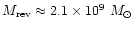
The mass of the black hole in 3C 390.3, estimated from the reverberation analysis is
.
The mass of the black hole in 3C 390.3, estimated from the reverberation analysis is
 ,
5 times larger than
previous estimates (Wandel et al. 1999).
,
5 times larger than
previous estimates (Wandel et al. 1999).
Key words: galaxies: active - galaxies: Seyfert - galaxies: individual (3C 390.3) - line: profiles
Long temporal baseline spectral monitoring of the nuclei of some AGNs has revealed a time lag in the response of the broad emission lines relative to flux changes of the continuum. This lag depends on the size, geometry and physical conditions of the emitting region. Thus, the search for correlations between nuclear continuum changes and flux variations of the broad emission lines may serve as a tool for mapping the geometrical and dynamical structure of the BLR (see Peterson 1993 and references therein). From the study of the responses of lines of different ions to changes of the nuclear continuum and the comparison of these data with photoionization model predictions, one could infer some of the physical conditions in the BLR as a function of the distance from the central source (Dumont et al. 1998).
From changes of the broad emission line profiles, we could distinguish, in principle, different kinematical models for the BLRs, including cases in which matter is undergoing accelerated motions, ie. falling or outflowing, Keplerian rotation in the gravitational field of the central body, etc. (Bochkarev & Antokhin 1982; Blanford & McKee 1982; Antokhin & Bochkarev 1983).
During the last decade, the study of the BLRs in some objects has met with considerable success, mainly due to an increasing number of coordinated multiwavelength monitoring campaigns through the international "AGN Watch'' program. This program has provided data with good temporal frequency and coverage for a number of selected Seyfert galaxies: NGC 5548 (Clavel et al. 1991; Peterson et al. 1991, 1993, 1994, 1999; Maoz et al. 1993; Dietrich et al. 1993; Korista et al. 1995; Chiang et al. 2000); NGC 3783 (Reichert et al. 1994; Stirpe et al. 1994; Alloin et al. 1995); NGC 4151 (Crenshaw et al. 1996; Kaspi et al. 1996; Warwick et al. 1996; Edelson et al. 1996); Fairall 9 (Rodriguez-Pascual et al. 1997; Santos-Lleo et al. 1997); NGC 7469 (Wanders et al. 1997; Collier et al. 1998) and 3C 390.3 (Leighly et al. 1997; Dietrich et al. 1998; O'Brien et al. 1998). It has been found that a significant part of the BLR variability can be associated with a region located within some light weeks from the central source. The infered BLR extent is comparable to the size of a hypothetical accretion disk surrounding a supermassive black hole. Therefore, at least part of the flux from the BLR arises, apparently, from the accretion disk itself (Laor & Netzer 1989; Dumont & Collin-Souffrin 1990a, 1990b; Zheng et al. 1991; Hubeny et al. 2000). It is also found that the higher ionization lines respond faster to continuum flux changes than those of lower ionization, while the optical and ultraviolet continua vary without a significant time lag between them.
The results of the studies of the velocity fields in the central sources are
still ambiguous. It is not clearly established yet, whether or not the time lags
in the response of the blue and red wings and the core of the line profile
with respect to continuum variations are the same. So far, studies of the
velocity-dependent response of the C IV  1549 emission line in
NGC 5548 have found no evidence of significant radial motions in its
BLR, (Korista et al. 1995).
1549 emission line in
NGC 5548 have found no evidence of significant radial motions in its
BLR, (Korista et al. 1995).
Most of the objects included in the multiwavelength monitoring
AGN Watch are radio-quiet Sy1 galaxies and only one, 3C 390.3
(z=0.0561), is a well-known broad line radiogalaxy. This type of
object represents about 10% of the radio-loud AGNs. It
is also a powerful double-lobed FRII radio-galaxy with a
relatively strong compact core. The two extended lobes, at a
position angle of 144 ,
each one with a hot spot, are
separated by about 223
,
each one with a hot spot, are
separated by about 223
 (Leahy & Perley 1991). A faint
well-collimated thin jet at PA = 37,
connecting the
core to the northern lobe, has been observed by Leahy & Perley
(1995). The VLBI observations at 5 GHz show evidence of
superluminal motion (with
(Leahy & Perley 1991). A faint
well-collimated thin jet at PA = 37,
connecting the
core to the northern lobe, has been observed by Leahy & Perley
(1995). The VLBI observations at 5 GHz show evidence of
superluminal motion (with
 )
in this parsec scale jet
(Alef et al. 1996, 1988).
)
in this parsec scale jet
(Alef et al. 1996, 1988).
The strong variability of this object, both in the continuum light and the
emission lines, is well known (Barr et al. 1980; Yee & Oke
1981; Netzer 1982; Barr et al. 1983;
Penston & Perez 1984; Clavel & Wamsteker 1987;
Veilleux & Zheng 1991; Shapovalova et al.
1996;
Zheng 1996; Wamsteker et al. 1997;
Dietrich et al. 1998; O'Brien et al. 1998). The
object is also a highly variable X-ray source, with a spectrum
showing a broad Fe K line (Inda et al. 1994;
Eracleous et al. 1996; Wozniak et al. 1998).
During a multiwavelength monitoring campaign in 1995, several large-amplitude
X-ray flares were observed in 3C 390.3; in one of them the flux increased
by a factor of 3 in only 12 days (Leighly et al. 1997). Furthermore,
Leighly & O'Brien (1997) have presented evidence for
nonlinear X-ray variability.
line (Inda et al. 1994;
Eracleous et al. 1996; Wozniak et al. 1998).
During a multiwavelength monitoring campaign in 1995, several large-amplitude
X-ray flares were observed in 3C 390.3; in one of them the flux increased
by a factor of 3 in only 12 days (Leighly et al. 1997). Furthermore,
Leighly & O'Brien (1997) have presented evidence for
nonlinear X-ray variability.
In an analysis of IUE spectra of 3C 390.3, obtained during the
1978-1986 period, Clavel & Wamsteker (1987) detected a
variability time lag of 50 and 60 days between the broad emission lines
of C IV 1549 and Ly,
and the
UV-continuum. However, from a reanalysis of the same
spectral data, Wamsteker et al. 1997 have derived a lag
of 116  60 days for C IV and 143 60 days for Ly.
Furthermore, from IUE monitoring data for December 1994 to
March 1996, O'Brien et al. (1998) obtained a corresponding
lag of 35 days for the C IV
60 days for C IV and 143 60 days for Ly.
Furthermore, from IUE monitoring data for December 1994 to
March 1996, O'Brien et al. (1998) obtained a corresponding
lag of 35 days for the C IV
 emission line and 60
days for Ly.
Yet, from optical monitoring of 3C 390.3 in the
1994-1995 period, Dietrich et al. (1998) derived a time
lag of about 20 days for the Balmer lines response to changes in the X-ray
continuum. At that time, no
temporal lag between the optical and the UV or X-ray continua
changes was detected. The UV-bump, usually observed in a large
number of Seyfert galaxies, is very weak or even absent in 3C 390.3
(Wamsteker et al. 1997). Our object is a prototype
of a class that shows very broad, double-peaked emission line profiles;
to explain this profile, a number of possible scenarios have been
suggested. These models address the following hypothetical physical
models:
emission line and 60
days for Ly.
Yet, from optical monitoring of 3C 390.3 in the
1994-1995 period, Dietrich et al. (1998) derived a time
lag of about 20 days for the Balmer lines response to changes in the X-ray
continuum. At that time, no
temporal lag between the optical and the UV or X-ray continua
changes was detected. The UV-bump, usually observed in a large
number of Seyfert galaxies, is very weak or even absent in 3C 390.3
(Wamsteker et al. 1997). Our object is a prototype
of a class that shows very broad, double-peaked emission line profiles;
to explain this profile, a number of possible scenarios have been
suggested. These models address the following hypothetical physical
models:
at +1500 kms-1, and determined from
the radial velocity changes a possible period of about 300
years that corresponds to 7 10
10
 for the BHs.
However, Eracleous et al. (1997), having added data on the
displacement of the H
blue peak for the 1988-1996 lapse,
obtained a period for the binary BH, P > 800 years, with an
estimated total mass for the binary BH larger than 10
for the BHs.
However, Eracleous et al. (1997), having added data on the
displacement of the H
blue peak for the 1988-1996 lapse,
obtained a period for the binary BH, P > 800 years, with an
estimated total mass for the binary BH larger than 10
 .
These authors argued that such a large value for the mass
of the BH is difficult to reconcile with the fact that the BHs found
so far in the centers of galaxies, have masses lower than
.
These authors argued that such a large value for the mass
of the BH is difficult to reconcile with the fact that the BHs found
so far in the centers of galaxies, have masses lower than
 .
Therefore, they reject the hypothesis of a binary black hole
for 3C 390.3.
.
Therefore, they reject the hypothesis of a binary black hole
for 3C 390.3.
and C IV 1549 blue wings lagged behind the red ones, implying
radial gas motions, this result is not confirmed
by Zheng (1996). Apparently, these contradictory results are caused by
the rather poor
temporal sampling of the UV data ( 94 days).
Dietrich et al. (1998) have not detected any lag in the response
of the blue and red wings relative to the core of Hand H
emission. It was also found that the
flux in the wings of H,
Ly
and C IV 1549
vary quasi-simultaneously (Shapovalova et al. 1996; O'Brien et al. 1998).
These results imply that there
are no significant radial motions in the BLR, and Livio & Xu (1997)
have shown that the double-peaked lines seen in 3C 390.3 cannot be produced
by two line-emitting streams, since the emission region
of the far cone jet would be obscured by the optically thick accretion disk.
94 days).
Dietrich et al. (1998) have not detected any lag in the response
of the blue and red wings relative to the core of Hand H
emission. It was also found that the
flux in the wings of H,
Ly
and C IV 1549
vary quasi-simultaneously (Shapovalova et al. 1996; O'Brien et al. 1998).
These results imply that there
are no significant radial motions in the BLR, and Livio & Xu (1997)
have shown that the double-peaked lines seen in 3C 390.3 cannot be produced
by two line-emitting streams, since the emission region
of the far cone jet would be obscured by the optically thick accretion disk.
)
accretion disk provides a good fit
to the broad H
and H
profiles (Rokaki et al. 1992). Simple disk
models predict two symmetrical bumps, the
blue bump being slightly brighter due to Doppler boosting effects. However, IUE data shows
a blue wing of Lymuch brighter than the red one this cannot be explained by
Doppler boosting effects alone. There are also epochs when the red wing
of Ly
is brighter than the blue one (Zheng 1996), i.e.
the flux ratio of the red to the blue wings is quite variable.
Also, quasiperiodic variations (
 yr) of the observed flux ratios of the
blue and red wings of Hhave been reported (Veilleux & Zheng 1991;
Shapovalova et al. 1996; Bochkarev et al.
1997a). In order to explain these variable ratios, more complex models are
required; for instance, hot spots
(Zheng et al. 1991); two-arm spiral waves in the
accretion disk (Chakrabarti & Wiita 1994); or a
relativistic eccentric disk (Eracleous et al. 1995).
yr) of the observed flux ratios of the
blue and red wings of Hhave been reported (Veilleux & Zheng 1991;
Shapovalova et al. 1996; Bochkarev et al.
1997a). In order to explain these variable ratios, more complex models are
required; for instance, hot spots
(Zheng et al. 1991); two-arm spiral waves in the
accretion disk (Chakrabarti & Wiita 1994); or a
relativistic eccentric disk (Eracleous et al. 1995).
Long temporal baseline studies of the changes in the broad emission line profile through systematic monitoring would allow us to distinguish between those models.
In this paper, we present the results of the spectral (H)
and photometric BVRI
monitoring of 3C 390.3 during
the 1995-1999 period. This work is part of the long-term
monitoring program for about 10 Seyfert galaxies of different
nuclear luminosities started in 1986 at the SAO RAS, and
carried out jointly, since 1998, with the INAOE (México), and several
observatories in the Former Soviet Union (FSU) and
West-European countries (Bochkarev et al. 1997b;
Bochkarev & Shapovalova 1999).
![\begin{figure}
\par\includegraphics[width=8.8cm,clip]{MS1186f1.eps} \end{figure}](/articles/aa/full/2001/36/aa1186/img27.gif) |
Figure 1:
The light curves of 3C 390.3 in the B, V and  photometric bands
for a 10
aperture, in the 1997-2000 period.
photometric bands
for a 10
aperture, in the 1997-2000 period. |
| Open with DEXTER | |
The BVR photometry of 3C 390.3 was carried out
at three different observatories i.e. SAO RAS in North
Caucasus (Russia), the Crimean Laboratory of the Sternberg Astronomical Institute (CL SAI, Russia)
and the Abastumani Astrophysical Observatory (AAO) in Georgia. The observations at
the SAO RAS during 1997-2000 were obtained with the 1 m and 60 cm Zeiss telescopes equipped
with an offset guided automatic photometer. The instrument
has a liquid nitrogen cooled CCD camera with a format of
 pixels,
(Amirkhanian et al. 2000). The scale at the CCD being 0.45
per pixel,
with a corresponding field of view of
pixels,
(Amirkhanian et al. 2000). The scale at the CCD being 0.45
per pixel,
with a corresponding field of view of
 arcmin.
Exposures of the morning and evening sky were used as
flat-field frames. Bias and dark current frames were also
obtained. Data reduction was carried out with the software
developed at SAO by Vlasyuk (1993). The photometry is obtained by
signal integration in concentric circular apertures, of increasing size,
centered at the baricenter of the measured object. The instrumental
photometric system of this instrument is similar to those of Johnson
in B and V, and of Cousins (1976) in R and I. The VRI photometry during 1998-1999 was
obtained at the Crimean Laboratory of the Sternberg Astronomical Institute
with the 60 cm telescope (Zeiss-600) equipped with an ST-6 thermoelectrically cooled CCD camera. The photometric system of CL SAI is similar to that of Johnson. Further details
about SAO and Crimean observations can be found in Doroshenko et al. (2001).
BVRI observations at the AAO in Georgia during 1997-1998 were obtained with the 70 cm
menisk telescope equipped with a CCD camera.
These data were reduced with the IRAF package (DAOPHOT).
arcmin.
Exposures of the morning and evening sky were used as
flat-field frames. Bias and dark current frames were also
obtained. Data reduction was carried out with the software
developed at SAO by Vlasyuk (1993). The photometry is obtained by
signal integration in concentric circular apertures, of increasing size,
centered at the baricenter of the measured object. The instrumental
photometric system of this instrument is similar to those of Johnson
in B and V, and of Cousins (1976) in R and I. The VRI photometry during 1998-1999 was
obtained at the Crimean Laboratory of the Sternberg Astronomical Institute
with the 60 cm telescope (Zeiss-600) equipped with an ST-6 thermoelectrically cooled CCD camera. The photometric system of CL SAI is similar to that of Johnson. Further details
about SAO and Crimean observations can be found in Doroshenko et al. (2001).
BVRI observations at the AAO in Georgia during 1997-1998 were obtained with the 70 cm
menisk telescope equipped with a CCD camera.
These data were reduced with the IRAF package (DAOPHOT).
As a local photometric standard, we adopted stars "B'' and "D''
of Penston et al. (1971) which are close to 3C 390.3 in our CCD images.
Consequently, effects due to differential air mass are negligible for internal
calibration purposes. The adopted BVRI magnitudes for the reference stars are given in Table  .
.
| Star | Ba | Va | Rb | Ib |
| B | 15.04 | 14.28 | 14.13 | 13.59 |
| D | 15.40 | 14.65 | 14.42 | 13.90 |
The results of the broad-band photometry of 3C 390.3
in the
 filters for a circular aperture of 10
obtained at AAO and CL SAI were transformed to the
SAO BVR photometric system. Our results are presented in graphical form in Fig.
filters for a circular aperture of 10
obtained at AAO and CL SAI were transformed to the
SAO BVR photometric system. Our results are presented in graphical form in Fig.  .
The estimated mean errors in the BVRI
photometry for the entire data set are 0.026, 0.021, 0.020, 0.022 magnitudes, respectively.
In Table
.
The estimated mean errors in the BVRI
photometry for the entire data set are 0.026, 0.021, 0.020, 0.022 magnitudes, respectively.
In Table
 our photometric results and the
corresponding errors are listed. The last column lists
the observatory where the data was obtained i.e. (SAO, SAI - Crimean
Laboratory, Abast. - Abastumani Astrophysical Observatory in Georgia).
our photometric results and the
corresponding errors are listed. The last column lists
the observatory where the data was obtained i.e. (SAO, SAI - Crimean
Laboratory, Abast. - Abastumani Astrophysical Observatory in Georgia).
![\begin{figure}
\par\includegraphics[width=12cm]{MS1186f2.eps}\end{figure}](/articles/aa/full/2001/36/aa1186/img34.gif) |
Figure 2: A historical light curve for 3C 390.3. Open cicles - Sandage (1973), Neizvestny (1986); large filled circles - photometry (present paper); open squares - Yee & Oke (1981); small filled circles - Babadzhanyants et al. (1973, 1974, 1975, 1976, 1984); crosses - Cannon et al. (1971), Scott et al. (1976), Selmes et al. (1975), Pica et al. (1980); plusses - spectral continuum (present paper); open triangles - Dietrich et al. (1998); filled triangles - spectral continuum from Perez et al. (1988) and Lawrence et al. (1996). |
| Open with DEXTER | |
| Table 2 is only available in electronic form at the CDS via anonymous ftp to cdsarc.u-strasbg.fr (130.79.128.5) or via http://cdsweb.u-strasbg.fr/cgi-bin/qcat?J/A+A/376/775 |
Spectra of 3C 390.3 were obtained with the 6 m and 1 m
telescopes of the SAO RAS (Russia, 1995-1999) and at INAOE's
2.1 m telescope of the "Guillermo Haro Observatory'' (GHO) at Cananea,
Sonora, México (1998-1999). The spectra were obtained with long slit
spectrographs equipped with CCD detector arrays. The typical
wavelength interval covered is from 4000 Å to 7500 Å. The
spectral resolution varied between 4 and 15 Å. Spectrophotometric
standard stars were observed every night. The specific information
about the instrumental set-ups for different telescopes is listed
in Table
 ,
where we list: 1 - telescope; 2 - type of
focus; 3 - spectrograph; 4 - CCD format; 5 - set-up code.
The log of spectroscopic observations is given in Table
,
where we list: 1 - telescope; 2 - type of
focus; 3 - spectrograph; 4 - CCD format; 5 - set-up code.
The log of spectroscopic observations is given in Table
 ,
listed in Col. 1 - UT date; 2 - Julian date; 3 - code according
to Table 3; 4 - projected spectrograph entrance
apertures (the first dimension being the slit-width, and
the second one the slit-length); 5 - wavelength range covered; 6 - spectral resolution; 7 - seeing; 8 - signal
to noise ratio in a region of the continuum (5370-5420 Å) where there are no
prominent emission or absorption lines.
The spectrophotometric data reduction was carried out either with software
developed at SAO RAS by Vlasyuk (1993) or with the IRAF package for the spectra
obtained in México. The image reduction process included bias,
flat-field corrections, cosmic ray removal, 2D wavelength
linearization, background subtraction, stacking of the spectra for
every set up, and flux calibration.
,
listed in Col. 1 - UT date; 2 - Julian date; 3 - code according
to Table 3; 4 - projected spectrograph entrance
apertures (the first dimension being the slit-width, and
the second one the slit-length); 5 - wavelength range covered; 6 - spectral resolution; 7 - seeing; 8 - signal
to noise ratio in a region of the continuum (5370-5420 Å) where there are no
prominent emission or absorption lines.
The spectrophotometric data reduction was carried out either with software
developed at SAO RAS by Vlasyuk (1993) or with the IRAF package for the spectra
obtained in México. The image reduction process included bias,
flat-field corrections, cosmic ray removal, 2D wavelength
linearization, background subtraction, stacking of the spectra for
every set up, and flux calibration.
| Telescope | Focus | Equipm. | CCD | Code |
| (pixels) | ||||
| 1 | 2 | 3 | 4 | 5 |
| 6 m SAO | Prime | UAGS |
 |
G |
| 6 m SAO | Prime | UAGS |
 |
P |
| 6 m SAO | Prime | MPFS |
|
T |
| 6 m SAO | Nasmyth | Long slit |
|
N |
| 1 m Zeiss | Cassegrain | UAGS |
|
Z1 |
| 1 m Zeiss | Cassegrain | UAGS |
 |
Z2 |
| 2.1 m GHO | Cassegrain | B&Ch |
|
M |
MPFS refers to a Multi-Pupil Field Spectrograph.
| Table 4 is only available in electronic form at the CDS via anonymous ftp to cdsarc.u-strasbg.fr (130.79.128.5) or via http://cdsweb.u-strasbg.fr/cgi-bin/qcat?J/A+A/376/775 |
![\begin{figure}
\par\includegraphics[width=8.8cm,clip]{MS1186f3.eps}\end{figure}](/articles/aa/full/2001/36/aa1186/img43.gif) |
Figure 3: The spectra corresponding to the high activity (top) and the low activity (bottom) states. |
| Open with DEXTER | |
Since, even under good photometric conditions, the accuracy of
spectrophotometric measurements is rarely better than 10%, for the study
of AGN variability the standard scheme for flux calibration by means of comparison
with stars of
known spectral energy distribution is not acceptable.
Instead, we use the flux of the narrow forbidden emission lines which in AGNs
are non-variable in time-scales of tens of
years. This is largely due to the extension of the narrow line
emitting region (NLR) and to the lower gas density present in it.
Thus, the effects of light traveling through this region,
together with the long recombination times
 years, for
 103 cm-3), damp out the short
time scale variability. Hence, the bright narrow emission lines are
usually adopted as internal calibration for scaling AGN spectra
(Peterson 1993). However, in the case of 3C 390.3 there has been
some discussion about the variability of these lines. Let us address
this question in more detail.
103 cm-3), damp out the short
time scale variability. Hence, the bright narrow emission lines are
usually adopted as internal calibration for scaling AGN spectra
(Peterson 1993). However, in the case of 3C 390.3 there has been
some discussion about the variability of these lines. Let us address
this question in more detail.
From IUE data, Clavel & Wamsteker (1987) found
that the flux in the narrow components of Lyand C IV 1549 emission lines in 3C 390.3 decreased
continuously by 40% between 1978 and 1986. The involved
time-scales suggest an upper limit of about 10 light years for the
size of the regions in which these lines are formed.
Zheng et al. (1995) reported a considerable variability of the
[O III] 4959 narrow emission line fluxes (1.8 times) from observations carried out between 1974 and 1990. We
believe that this result is somewhat doubtful in the light of
the following considerations: the variability is only infered when
comparing results from observations carried out with different
instrumental set-ups. They include, on the one hand, fluxes
from image dissector scanner (IDS) data, obtained with the Shane
3 m telescope at Lick Observatory through an aperture of
 (1974-1983 lapse) and on the other hand,
observations carried out at La Palma with the 2.5 m Isaac Newton
telescope (INT), equipped with an image photon counting system (IPCS)
through a 1.6
wide slit (1984-1989). The lowest flux values
largely correspond to those observed at La Palma through this rather
narrow slit. Hence, it is possible that the large differences in flux
reported for the [O III] 4959 line could be due to
effects associated with the narrow slit used. Furthermore, in the spectra published
by Zheng et al. (1995), it is clearly seen that, during 1988 and 1989,
the red wing of H
showed an important enhancement and its contribution
could have also affected the determination of the [O III] line
flux. Unfortunately, these authors do not provide a detailed
discussion of their adopted procedure for flux determination.
(1974-1983 lapse) and on the other hand,
observations carried out at La Palma with the 2.5 m Isaac Newton
telescope (INT), equipped with an image photon counting system (IPCS)
through a 1.6
wide slit (1984-1989). The lowest flux values
largely correspond to those observed at La Palma through this rather
narrow slit. Hence, it is possible that the large differences in flux
reported for the [O III] 4959 line could be due to
effects associated with the narrow slit used. Furthermore, in the spectra published
by Zheng et al. (1995), it is clearly seen that, during 1988 and 1989,
the red wing of H
showed an important enhancement and its contribution
could have also affected the determination of the [O III] line
flux. Unfortunately, these authors do not provide a detailed
discussion of their adopted procedure for flux determination.
Relevant in the context of forbidden line variability are the
observations by Yee & Oke (1981) that covered the 1969-1980
period; these were carried out with the Hale 5 m telescope using a
multichannel spectrophotometer through an aperture of 10
.
They found that the [O III] lines and the narrow Balmer line fluxes
did not change during those years. Also, a detailed study of the [O III] 5007 flux variability in 3C 390.3
was carried out by Dietrich et al. (1998) during 1994-1995. The spectra
were obtained through wide apertures (5
7.5
and 4
10
)
and were calibrated by comparison with broad band photometry.
It was found, as expected, that the [O III] 5007 line flux remained
constant
(within 2.6%)
during the observed time interval. Therefore, we consider that in the case of 3C 390.3
there is no reliable evidence of the [O III]
 4959+5007 flux
variability on
time scales of months to few years. Our spectra for the H
region were scaled by
the [O III]
4959+5007 integrated line flux under the assumption
that the latter did not change during the time interval covered by our observations
(1995-1999).
A value of
4959+5007 flux
variability on
time scales of months to few years. Our spectra for the H
region were scaled by
the [O III]
4959+5007 integrated line flux under the assumption
that the latter did not change during the time interval covered by our observations
(1995-1999).
A value of
 ergs-1cm-2 (Veilleux & Zheng 1991)
for the integrated [O III] line flux was adopted. In order to calculate a
normalization coefficient, the continuum was determined in two 30 Å wide
clean - line free - windows centered at 4800 Å and 5420 Årespectively.
After continuum subtraction, blend separation of the H
and [O III]
components was carried out by means of a Gaussian fitting procedure, applied to
the following: H - broad blue, broad red and central narrow; [O III]
4959, 5007 - broad and narrow components. The forbidden lines being
represented by two Gaussian curves with an intensity ratio I(5007)/I
(4959)=2.96.
ergs-1cm-2 (Veilleux & Zheng 1991)
for the integrated [O III] line flux was adopted. In order to calculate a
normalization coefficient, the continuum was determined in two 30 Å wide
clean - line free - windows centered at 4800 Å and 5420 Årespectively.
After continuum subtraction, blend separation of the H
and [O III]
components was carried out by means of a Gaussian fitting procedure, applied to
the following: H - broad blue, broad red and central narrow; [O III]
4959, 5007 - broad and narrow components. The forbidden lines being
represented by two Gaussian curves with an intensity ratio I(5007)/I
(4959)=2.96.
was determined from scaled
spectra after continuum subtraction and removal of the [O III]
doublet. The narrow component of H
was not subtracted due to possible ambiguities in the
fitting scheme for the broad and narrow components of
the line. The contribution of
the narrow component to the integral H
flux is only 7%.
As Peterson & Collins (1983) pointed out, it is necessary to correct
the fluxes for aperture effects, due to the fact that
while the BLR and nonstellar continuum are effectively pointlike
sources (<1
), the NLR is an extended one
(>2-15
). Then, the measured NLR flux depends on
the size of the spectrograph's entrance aperture, and in the
case of direct images, on the size of the adopted aperture. The light
contribution of the host galaxy to the continuum depends
also on the aperture size. Peterson et al. (1995) have
shown that
the uncertainties in CCD photometry can be minimized, when
sufficiently large apertures are adopted. For an aperture of
 ,
the expected photometric errors are typically 2 to 3%.
,
the expected photometric errors are typically 2 to 3%.
The NLR in 3C 390.3 is more compact
than in most Sy1 galaxies; in narrow-band [O III] images, this object
shows a compact nuclear emission without signs of an extended structure (Baum et al.
1988). The results of panoramic two-dimensional spectrophotometry
of the nuclear region of this object show that the [O III] 5007
emission arises from a zone smaller than r<2
(Bochkarev et al.
1997a). Furthermore, Osterbrock et al. (1975) obtained a
rather low value for the
[O III] F(4363)/F(5007) line ratio, implying
a moderately high electron density in the NLR (several 106 cm-3).
Since the NLR in 3C 390.3 can be considered as a point
source, we did not apply corrections for aperture
effects to the nonstellar continuum, the narrow line flux ratios or
the broad to narrow line flux ratios. As the light losses in
the slit are similar for these components. However,
the light contribution to the continuum from the host galaxy does depend
on the aperture, and it is necessary to correct for this effect. To acomplish this goal,
we adopted the scheme by Peterson et al. (1995). It is based on the ratio:
![\begin{displaymath}F_{\rm con}=F(4959+5007)\left[\frac{F_{\rm con}}{F(4959+5007)}\right]_{\rm obs} - G,
\end{displaymath}](/articles/aa/full/2001/36/aa1186/img50.gif) |
(1) |
 ,
this
instrumental setup was adopted as the standard one (i.e. G=0 by definition). The
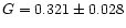
value of G for the spectra obtained at the 2.1 m telescope
(aperture of
,
this
instrumental setup was adopted as the standard one (i.e. G=0 by definition). The
value of G for the spectra obtained at the 2.1 m telescope
(aperture of
 )
is G=0.046, while the value
obtained for the 1 m telescope (aperture of
)
is G=0.046, while the value
obtained for the 1 m telescope (aperture of
 )
is
)
is
 .
In Table
.
In Table
 we list the derived values of the H
flux in
the 4990 Å to 5360 Å wavelength range, jointly with the continuum flux at 5125 Å.
The mean error (uncertainty) in our flux
determination for both the H
and the continuum is 3%. These
quantities were estimated by comparing results
from spectra obtained within a time interval shorter than 2 days.
we list the derived values of the H
flux in
the 4990 Å to 5360 Å wavelength range, jointly with the continuum flux at 5125 Å.
The mean error (uncertainty) in our flux
determination for both the H
and the continuum is 3%. These
quantities were estimated by comparing results
from spectra obtained within a time interval shorter than 2 days.
In Table
 we list our results, there one finds: 1 - The Julian date;
2 - a code, according to Table
we list our results, there one finds: 1 - The Julian date;
2 - a code, according to Table
 ;
3 - F(H)
the total
flux (in units of 10-13 ergs-1cm-2);
4 -
;
3 - F(H)
the total
flux (in units of 10-13 ergs-1cm-2);
4 -
 - the H
flux error; 5 -
- the H
flux error; 5 -  -
the continuum flux at 5125 Å(in units of 10-15 erg s-1 cm-2 A-1),
reduced to the 6 m telescope aperture
(2
6
); 6 -
-
the continuum flux at 5125 Å(in units of 10-15 erg s-1 cm-2 A-1),
reduced to the 6 m telescope aperture
(2
6
); 6 -
 - the estimated continuum flux error.
| JD | Code | F(H)
 |
|
 |
 |
| 2440000+ | |||||
| 49832.424 | G | 2.107 | 0.070 | 1.309 | 0.043 |
| 49863.375 | T | 2.715 | 0.090 | 1.576 | 0.052 |
| 50039.156 | G | 2.537 | 0.084 | 2.636 | 0.087 |
| 50051.143 | G | 2.840 | 0.094 | 2.703 | 0.089 |
| 50052.149 | G | 2.368 | 0.078 | 2.923 | 0.097 |
| 50127.602 | N | 3.073 | 0.101 | 2.529 | 0.084 |
| 50162.580 | N | 3.335 | 0.110 | 2.571 | 0.085 |
| 50163.553 | N | 3.502 | 0.116 | 2.756 | 0.091 |
| 50249.542 | G | 2.937 | 0.097 | 1.851 | 0.061 |
| 50276.567 | G | 3.202 | 0.106 | 1.638 | 0.054 |
| 50277.556 | G | 2.961 | 0.098 | 1.681 | 0.056 |
| 50281.434 | G | 2.775 | 0.092 | 1.607 | 0.053 |
| 50305.489 | G | 2.908 | 0.096 | 1.813 | 0.060 |
| 50338.319 | Z2 | 2.621 | 0.087 | 1.801 | 0.059 |
| 50390.435 | G | 2.459 | 0.081 | 1.592 | 0.053 |
| 50511.622 | G | 1.761 | 0.058 | 1.187 | 0.039 |
| 50599.370 | G | 1.729 | 0.057 | 1.167 | 0.039 |
| 50618.523 | G | 1.852 | 0.061 | 0.996 | 0.033 |
| 50656.499 | G | 1.585 | 0.052 | 0.922 | 0.030 |
| 50691.463 | G | 1.432 | 0.047 | 1.076 | 0.036 |
| 50701.576 | N | 1.301 | 0.043 | 1.160 | 0.038 |
| 50808.582 | G | 1.718 | 0.057 | 1.551 | 0.051 |
| 50813.195 | G | 1.638 | 0.054 | 1.580 | 0.052 |
| 50835.631 | N | 1.928 | 0.064 | 1.799 | 0.059 |
| 50867.560 | N | 2.080 | 0.069 | 1.685 | 0.056 |
| 50904.627 | G | 1.969 | 0.065 | 1.970 | 0.065 |
| 50940.354 | N | 2.535 | 0.084 | 1.832 | 0.060 |
| 50942.342 | N | 2.531 | 0.084 | 1.835 | 0.061 |
| 50990.302 | N | 2.481 | 0.082 | 1.748 | 0.058 |
| 51010.719 | M | 2.556 | 0.084 | 1.582 | 0.052 |
| 51019.723 | M | 2.544 | 0.084 | 1.408 | 0.047 |
| 51023.491 | G | 2.617 | 0.086 | 1.596 | 0.053 |
| 51025.431 | G | 2.370 | 0.078 | 1.408 | 0.047 |
| 51055.376 | N | 2.313 | 0.076 | 1.509 | 0.050 |
| 51074.506 | Z1 | 2.546 | 0.084 | 1.537 | 0.051 |
| 51081.429 | M | 2.250 | 0.074 | 1.508 | 0.050 |
| 51082.429 | M | 2.345 | 0.077 | 1.617 | 0.053 |
| 51083.429 | M | 2.413 | 0.080 | 1.570 | 0.052 |
| 51112.259 | G | 2.339 | 0.077 | 1.433 | 0.047 |
| 51130.169 | Z1 | 2.019 | 0.067 | 1.705 | 0.056 |
| 51372.516 | P | 1.610 | 0.053 | 1.163 | 0.038 |
| 51410.309 | P | 1.931 | 0.064 | 1.399 | 0.046 |
| 51426.208 | P | 1.784 | 0.059 | 1.393 | 0.046 |
| 51454.674 | M | 2.223 | 0.073 | 1.660 | 0.055 |
| 51455.172 | P | 2.111 | 0.070 | 1.415 | 0.047 |
| 51491.592 | M | 2.747 | 0.091 | 2.321 | 0.077 |

In order to construct a light curve in the B band
dating back to 1966, in addition to our photometric data for the 1997-2000
period, we
collected from the literature all the available photometry for 3C 390.3 reported
during
the last 30 years. We included the photoelectric observations, carried out in
1965-1967,
1971 and 1982 by Sandage (1973) and Neizvestny (1986);
spectrophotometric observations for 1970-1979 by Yee & Oke (1981),
from which we derived B magnitudes in excellent agreement with
contemporary photoelectric photometry. We also make use of the photographic
photometry available, i.e. 1967-1980 from Cannon et al. (1971);
Babadzhanyants et al. (1973, 1974, 1975, 1976,
1984);
Selmes et al. (1975); Scott et al. (1976); Pica
et al. (1980). In order to increase their accuracy, the photographic
observations were
averaged in 5 day
bins. We also included a few spectral observations by Pérez et al.
(1988),
Lawrence et al. (1996) and the International Monitoring data in
the framework of the AGN Watch consortium for 1994-1995 (Dietrich et al.
1998) and spectral
continuum light curve data, discussed here. The resulting
light curve in B band is shown in Fig.  .
There, we can see a
noticeable increase in luminosity with significant fluctuations between 1965
and 1977. The amplitude of the outburst from the middle of 1969 until the
middle of 1970 was about
.
There, we can see a
noticeable increase in luminosity with significant fluctuations between 1965
and 1977. The amplitude of the outburst from the middle of 1969 until the
middle of 1970 was about  .
In 1979 the brightness of 3C 390.3 decreased
to
.
In 1979 the brightness of 3C 390.3 decreased
to
 and remained at this level until 1983. At that time,
Penston & Pérez (1984) noted that the broad component of
H
had disappeared, and the spectrum of the object became quite similar to
that of a Sy2 galaxy. A similar behavior was observed in NGC 4151,
for which, after a long-lasting photometric minimum between 1984 and 1989 the
broad wings of H
also disappeared and was then classified as Sy2 at that
time (Penston & Pérez 1984; Lyuty et al. 1984). In the
case of 3C 390.3, after maximum light
in 1970, on the descending branch of the light curve, important oscillations
with an amplitude up to
and remained at this level until 1983. At that time,
Penston & Pérez (1984) noted that the broad component of
H
had disappeared, and the spectrum of the object became quite similar to
that of a Sy2 galaxy. A similar behavior was observed in NGC 4151,
for which, after a long-lasting photometric minimum between 1984 and 1989 the
broad wings of H
also disappeared and was then classified as Sy2 at that
time (Penston & Pérez 1984; Lyuty et al. 1984). In the
case of 3C 390.3, after maximum light
in 1970, on the descending branch of the light curve, important oscillations
with an amplitude up to  were observed. Unfortunately, we have not found
photometric observations of this object for the 1983-1993 period and
hence, the photometric behavior of 3C 390.3 during this
period of time is unknown. A detailed study of the character of the visible
light variability in 3C 390.3 will be presented in a separate paper.
were observed. Unfortunately, we have not found
photometric observations of this object for the 1983-1993 period and
hence, the photometric behavior of 3C 390.3 during this
period of time is unknown. A detailed study of the character of the visible
light variability in 3C 390.3 will be presented in a separate paper.
 emission line and the
optical continuum
emission line and the
optical continuum
The photometric data obtained during 1997-2000 is plotted in
Fig.  .
The light curve shows an almost sinusoidal change
in brightness with a maximum amplitude of about
.
The light curve shows an almost sinusoidal change
in brightness with a maximum amplitude of about
 in the B band. Brightness
maxima ocurred in May-June 1998 and in March-April 2000.
The light curves in the V and R
bands are similar in shape to those of the B band, but have a smaller
amplitude (
in the B band. Brightness
maxima ocurred in May-June 1998 and in March-April 2000.
The light curves in the V and R
bands are similar in shape to those of the B band, but have a smaller
amplitude (
 ),
as expected from a blue variable continuum.
In Fig.
),
as expected from a blue variable continuum.
In Fig.  ,
one can also notice small amplitude light
fluctuations, superimposed on longer time-scale changes.
Between 1995 and 1999 the H
flux changes reached a
maximum amplitude of 2.7, while those of the continuum at
5125 Å show a maximum amplitude of 3.2 (Table
,
one can also notice small amplitude light
fluctuations, superimposed on longer time-scale changes.
Between 1995 and 1999 the H
flux changes reached a
maximum amplitude of 2.7, while those of the continuum at
5125 Å show a maximum amplitude of 3.2 (Table
 ).
These changes are evident in a simple inspection of the spectrum of the high-activity (Fig.
).
These changes are evident in a simple inspection of the spectrum of the high-activity (Fig.  )
state (20 Mar. 1996) as compared with corresponding one of the low-activity state (9 Sep. 1997).
From the combined light curve (Fig.
)
state (20 Mar. 1996) as compared with corresponding one of the low-activity state (9 Sep. 1997).
From the combined light curve (Fig.  )
for the 1995-1999 time interval, we confirm a maximum amplitude flux variation in B of 3.2. This value is in excellent agreement with the value derived from
spectroscopic continuum fluxes, rendering further support to our basic assumption: i.e.
that the flux of the [O III] lines did not change during the period of time
covered by our observations.
)
for the 1995-1999 time interval, we confirm a maximum amplitude flux variation in B of 3.2. This value is in excellent agreement with the value derived from
spectroscopic continuum fluxes, rendering further support to our basic assumption: i.e.
that the flux of the [O III] lines did not change during the period of time
covered by our observations.
![\begin{figure}
\par\includegraphics[width=8.6cm,clip]{MS1186f4.eps}\end{figure}](/articles/aa/full/2001/36/aa1186/img76.gif) |
Figure 4:
3C 390.3 Light curves of the H
(panel a)) and the 5125 Å optical continuum emission
(panel b)) during 1995-2000. Filled
circles represent the spectral data. The photometric points are
represented by open circles. Units are 10-13 ergcm-2s-1 for H
fluxes and 10-15 ergcm-2s-1A-1) for the continuum ones.
In panel c) we plot -
 -
-
 ,
the velocity difference
of the peak emission of the red and blue bumps (in km s-1), derived from the H
difference profiles. ,
the velocity difference
of the peak emission of the red and blue bumps (in km s-1), derived from the H
difference profiles. |
| Open with DEXTER | |
Figures
 a and b show the light curves for
the integrated H (4990-5360 Å) and continuum (5125 Å) fluxes.
In order to improve the time resolution of our continuum
data set, we have added some photometric points in the V band to our spectral
continuum data. The V band data
was converted into flux adopting the calibration by Johnson (1966). A
comparison of the spectral continuum photometry at 5125 Å ((5125))
with 10 simultaneous observations in the V band yields the following
transformation equation:
a and b show the light curves for
the integrated H (4990-5360 Å) and continuum (5125 Å) fluxes.
In order to improve the time resolution of our continuum
data set, we have added some photometric points in the V band to our spectral
continuum data. The V band data
was converted into flux adopting the calibration by Johnson (1966). A
comparison of the spectral continuum photometry at 5125 Å ((5125))
with 10 simultaneous observations in the V band yields the following
transformation equation:
 |
(2) |
In Figs.
 a and b two outbursts in H
and the
continuum are evident, with time intervals between minima of 1000 days (Oct. 1994 - Jul. 1997) and 700 days (Jul. 1997 - Jun. 1999), respectively.
Also, the presence of a time lag between the continuum light changes
and the response of the H
line, is also noticeable.
a and b two outbursts in H
and the
continuum are evident, with time intervals between minima of 1000 days (Oct. 1994 - Jul. 1997) and 700 days (Jul. 1997 - Jun. 1999), respectively.
Also, the presence of a time lag between the continuum light changes
and the response of the H
line, is also noticeable.
In Fig.
 ,
panels a,b,c and d show the derived correlations between
the continuum and H
light curves, for time lags between the continuum
and line variations of 0, 20, 40 and 100 days respectively. There, it is clear
that the variance of the data is
minimal and the correlation coefficient is maximal (r=0.94) for
a delay of 100 days. For this case, we obtained the following relationship:
,
panels a,b,c and d show the derived correlations between
the continuum and H
light curves, for time lags between the continuum
and line variations of 0, 20, 40 and 100 days respectively. There, it is clear
that the variance of the data is
minimal and the correlation coefficient is maximal (r=0.94) for
a delay of 100 days. For this case, we obtained the following relationship:
 |
(3) |
(5125)
fluxes are expressed in units of
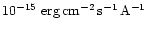 and the
 )
fluxes in units of
)
fluxes in units of
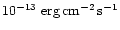 .
The values chosen for the delays are typical values previously
mentioned in the literature.
In Sect. 3.4 we present a detailed discussion
of the delays from a cross-correlation analysis of our data.
.
The values chosen for the delays are typical values previously
mentioned in the literature.
In Sect. 3.4 we present a detailed discussion
of the delays from a cross-correlation analysis of our data.
![\begin{figure}
\par\includegraphics[width=8.8cm,clip]{MS1186f5.eps}\end{figure}](/articles/aa/full/2001/36/aa1186/img85.gif) |
Figure 5:
The F(H)
and (5125) plotted
against each other. In panels a-d)
these quantities are plotted taking into account a time lag of 0, 20 , 40 and 100 days, respectively. The correlation coefficients for the linear
regressions are also given. |
| Open with DEXTER | |
![\begin{figure}
\par\includegraphics[width=8.6cm,clip]{MS1186f6.eps} \end{figure}](/articles/aa/full/2001/36/aa1186/img86.gif) |
Figure 6:
The line light curves. a-c) for the blue wing in the
5010-5099 Å (-7100 kms-1 to -1900 kms-1) interval, for
the core
in the 5099-5164 Å (-1900 kms-1 to +1900 kms-1) interval,
and for the red wing of the broad H
emission
in the 5164-5253 Å (+1900 kms-1 to +7100 kms-1) interval,
respectively. Panel d) shows the temporal behavior of the blue-to-red wing flux
ratio R. |
| Open with DEXTER | |
wings
In order to investigate the flux in the different parts of the Hprofile, we studied three different velocity bins: a blue
wing ( kms-1 to
  kms-1), a core (-1900 kms-1
to +1900 kms-1) and a red wing (+1900 kms-1 to +7100 kms-1). The
light curves for these are presented in Figs.
kms-1), a core (-1900 kms-1
to +1900 kms-1) and a red wing (+1900 kms-1 to +7100 kms-1). The
light curves for these are presented in Figs.
 a-c,
where we can see that the changes in both the blue and red wings and the core occur
quasi-simultaneously. This fact implies that there are predominantly circular
motions in the region where the broad H
emission originates. The blue-to-red
wing flux ratio R is plotted in Fig.
a-c,
where we can see that the changes in both the blue and red wings and the core occur
quasi-simultaneously. This fact implies that there are predominantly circular
motions in the region where the broad H
emission originates. The blue-to-red
wing flux ratio R is plotted in Fig.
 d. Veilleux & Zheng (1991) noticed that between 1974 and
1988, the blue-to-red wing flux ratio followed a fairly smooth, almost
sinusoidal pattern with an apparent period of 10.4 years. This
trend was confirmed by Bochkarev et al.(1997a) with observations
that extended until 1995. Although maxima for the ratio R were observed in the
years: 1975, 1985, and 1995, the sinusoidal trend of R did not continue during the 1996-1999 period. In Fig.
d. Veilleux & Zheng (1991) noticed that between 1974 and
1988, the blue-to-red wing flux ratio followed a fairly smooth, almost
sinusoidal pattern with an apparent period of 10.4 years. This
trend was confirmed by Bochkarev et al.(1997a) with observations
that extended until 1995. Although maxima for the ratio R were observed in the
years: 1975, 1985, and 1995, the sinusoidal trend of R did not continue during the 1996-1999 period. In Fig.
 d, it is
evident that R continued to increase in a nearly monotonic fashion between 1995 and 1999.
d, it is
evident that R continued to increase in a nearly monotonic fashion between 1995 and 1999.
broad and continuum emissions
In order to determine a more accurate time lag than the one
described in 3.2, we carried out
a time series analysis using the cross-correlation function (CCF).
The CCF was calculated by means of the
interpolation method described by Gaskell & Sparke (1986) and
White & Peterson (1994). We
computed both the lags related to the CCF peak (
 )
and
the CCF centroid (
)
and
the CCF centroid (
 ). The value of (
)
is that of the center of mass of the CCF for
positive delay values. The CCF is calculated by pairing each of the real data points in both time-series with
linearly interpolated points for any arbitrary time delay.
). The value of (
)
is that of the center of mass of the CCF for
positive delay values. The CCF is calculated by pairing each of the real data points in both time-series with
linearly interpolated points for any arbitrary time delay.
According to Gaskell & Peterson (1987) not every time series is suitable for the cross-correlation analysis, only those series for which the autocorrelation function (ACF) width is wider (by at least 10%) than the width of the corresponding function for the sampling window (ACFW), contain relevant information about time lags. The ACFW is computed by repeated sampling of white noise light curves, convolved with the observational window. This procedure provides a measure of how much of the width of the ACF is due to the interpolating scheme, instead of the real correlation width of a continuous time series sampled at discrete times. In addition, the half width of the ACF at a zero correlation level determines the characteristic size of the region from which variations originate, setting an upper limit to the BLR size.
The ACFW was calculated for the time series of the
observations, upon which random Gaussian noise corresponding to
the observing
errors in the time series was superimposed. The mean ACFW for one
hundred of
those realizations
is shown in Fig.  a. There we can see that the
ACFW is much narrower than the ACF for either the continuum or
the H
emissions.
a. There we can see that the
ACFW is much narrower than the ACF for either the continuum or
the H
emissions.
![\begin{figure}
\par\includegraphics[width=8.8cm,clip]{MS1186f7.eps}\end{figure}](/articles/aa/full/2001/36/aa1186/img95.gif) |
Figure 7:
The Auto- and Cross-Correlation
Functions. In panel a), the narrow curve represents the
sampling window autocorrelation function (ACFW) for the
spectral continuum and H
line. Also, the autocorrelation
functions (ACF) for the H
label (1) and the
continuum light curves (2) are shown. On panels b) and d), the CCFs for the periods 1995-1999
and 1997-1999 respectively are shown. Curves labeled (1) represent
the CCF between the H
flux and the spectral continuum at 5125 Å;
curves labeled (2) represent the CCF for the H
flux and the
combined continuum and label (3) refers to the CCF computed as in
case (2), but for a restricted interpolation of 100 days. Panel c) shows the CCF between: (1) -
H
blue and red wings light curves , (2) - Hred wing and H
core fluxes and (3) - H
blue
wing and H
core light curves. In every panel the units
are: delay in days (abscissae) and correlation coefficient (ordinates). |
| Open with DEXTER | |
Usually, the time delay is determined either by the location
of the peak, or that of the center of mass of the
cross-correlation function between the continuum and the
emission line light curves. Robinson & Pérez (1990)
argued that the position of the CCF peak (
)
yields the
time delay corresponding to the inner radius of the BLR, while
the position of the center of mass of the CCF (
)
relates to the size of the BLR weighted by luminosity.
The errors in the determination of the time lags
were estimated
through a Monte Carlo
simulation. From 1000 independent realizations of the CCF, the
and
distributions were obtained. Prior to the
computation, the time-series involved were corrupted with
Gaussian noise corresponding to the typical errors in them.
Cutting the distribution functions at a 17% probability level,
the uncertainty related to a 67% confidence level (1 error) was determined.
During the International Monitoring Programme of the Sy galaxy NGC 5548, for a period of 8 years, it was observed by Peterson et al. (1999) that the time lag in this object does not have a constant value, and that changes of the delay may be related to the luminosity variations of the central source. During the time interval cover by our observations, the photometric and spectral light curves of 3C 390.3 show two distinct flares. It is then important to determine the delays not only for the entire time-series, but also for the segments of it that correspond to relevant events in the light curves. Therefore, analysis of the light curves was carried out for various cases, as follows:
The CCF analysis has been carried out separately for the entire data set
- case A (
 ), and for the two sub-sets
(cases B,
), and for the two sub-sets
(cases B,
 ;
and C,
;
and C,
 ). It should be
mentioned that for case B, we do not have supplementary photometry,
while in case C we included our broad band photometry.
For this reason, the flux cross-correlation was calculated
not only for the spectral continuum fluxes
). It should be
mentioned that for case B, we do not have supplementary photometry,
while in case C we included our broad band photometry.
For this reason, the flux cross-correlation was calculated
not only for the spectral continuum fluxes
 ,
but also for the combined continuum data
,
but also for the combined continuum data
 .
To the latter, we added our photometric data in the V band to the spectral
continuum data as discussed above in Sect. 3.2.
.
To the latter, we added our photometric data in the V band to the spectral
continuum data as discussed above in Sect. 3.2.
Since many spectral observations were obtained with long time intervals between them, the CCF was calculated restricting the interpolation processes to time intervals no longer than 100 days (cases - AD, CD). That is, prior to the CCF computation, both time series were analyzed as to whether or not they were suitable for pairing. With this 100 day restriction in the pairing, possible effects associated with long time gaps are reduced.
![\begin{figure}
\par\includegraphics[height=20.4cm,width=15.4cm,clip]{MS1186f8.eps}\end{figure}](/articles/aa/full/2001/36/aa1186/img102.gif) |
Figure 8:
Typical broad H
profiles (solid line) after
continuum and narrow components subtraction (dashed line). |
| Open with DEXTER | |
The results of the cross-correlation analysis
are presented in Fig.  and summarized
in Table
and summarized
in Table
 .
There we list: in Col. 1 the time-series case;
in Col. 2 - the cross-correlation case: (F(H)
-
)
- between
the continuum F(5125) and H
fluxes; (F(H)
-
)
- between the combined continuum
and H
fluxes; in Col. 3 -
- the time lag in days,
determined from the position of the CCF maxima; in Col. 4 - 1
interval for
;
in Col. 5 -
.
There we list: in Col. 1 the time-series case;
in Col. 2 - the cross-correlation case: (F(H)
-
)
- between
the continuum F(5125) and H
fluxes; (F(H)
-
)
- between the combined continuum
and H
fluxes; in Col. 3 -
- the time lag in days,
determined from the position of the CCF maxima; in Col. 4 - 1
interval for
;
in Col. 5 -
 - the cross-correlation coefficient for the CCF maxima;
in Col. 6 -
- the time lag in days, determined from the centroids
of the CCF; in Col. 7 - the estimated 1
uncertainty for
;
in Cols. 8 and 9 -
the number of points, used in the
computations - N(H)
and -
- the cross-correlation coefficient for the CCF maxima;
in Col. 6 -
- the time lag in days, determined from the centroids
of the CCF; in Col. 7 - the estimated 1
uncertainty for
;
in Cols. 8 and 9 -
the number of points, used in the
computations - N(H)
and -  .
.
| Time | Case |
|
1 |
|
|
1 |
N(H) |
|
| series | interv. | interv. | ||||||
| A | F(H)-
|
105 | 0.928 | 99 | 44 | 44 | ||
| A | F(H)-
|
100 | 97-101 | 0.900 | 86 | 79-92 | 44 | 127 |
| AD | F(H)-
|
99 | 0.930 | 98 | 37 | 45 | ||
| B | F(H)-
|
98 | 0.946 | 109 | 20 | 21 | ||
| B | F(H)-
|
99 | 93-113 | 0.954 | 112 | 98-114 | 20 | 29 |
| C | F(H)-
|
105 | 0.885 | 90 | 27 | 26 | ||
| 34 | 0.800 | |||||||
| C | F(H)-
|
34 | 33-37 | 0.829 | 63 | 50-72 | 27 | 109 |
| 99 | 97-119 | 0.784 | ||||||
| CD | F(H)-
|
99 | 0.859 | 78 | 24 | 33 | ||
| 33 | 0.803 | |||||||
| A | F(H)b-F(H)c |
0 | -3.7-1.2 | 0.809 | -1.6 | -5.0-1.2 | 44 | 44 |
| A | F(H)r-F(H)c |
-1.0 | -3.3-0.9 | 0.957 | -1.5 | -4.6-0.8 | 44 | 44 |
| A | F(H)b-F(H)r |
0.5 | -1.3-7.8 | 0.894 | 0.6 | -2.1-8.0 | 44 | 44 |
Inspection of Fig.  and
Table
and
Table
 ,
shows that:
,
shows that:
relative to the continuum flux changes
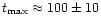 days or a little less for
 days;
days;
Our delay values differ from the results of Dietrich et al. (1998).
From Fig.
 one can
clearly see that the 20 day lag, obtained by these authors, yields
a much larger variance and a lower correlation coefficient between line
and continuum fluxes than the 100 day lag. In our data we do not see a lag
of 20 days or something similar. The reason for this discrepancy is
not clear to us. Perhaps it is related to the longer time interval
covered by our observations. It is conceivable that the time delay in
this object does not have a constant value, and that changes of the time
lag may be related to the luminosity variations of the central source.
A similar case for the Sy galaxy, NGC 5548, was studied by Peterson et al.
(1999).
one can
clearly see that the 20 day lag, obtained by these authors, yields
a much larger variance and a lower correlation coefficient between line
and continuum fluxes than the 100 day lag. In our data we do not see a lag
of 20 days or something similar. The reason for this discrepancy is
not clear to us. Perhaps it is related to the longer time interval
covered by our observations. It is conceivable that the time delay in
this object does not have a constant value, and that changes of the time
lag may be related to the luminosity variations of the central source.
A similar case for the Sy galaxy, NGC 5548, was studied by Peterson et al.
(1999).
profile
profile to
variations of the optical continuum. The delays found were 100-113
light days for
,
and 86-102 light days for
.
However, it
should be mentioned that 7% of the maxima in the distribution of the
CCF peak for the case of the F(H)
blue wing -
correspond to a delay of about 40 days, almost the same as in
case C previously discussed (see Sect. 3.4.1).
The possible differences in the response of the various parts
of the line profile can be studied through their
cross-correlation functions. In our case, the cross-correlation
of the blue-core, red-core and blue-red H
components are
presented in
Fig.  c. The corresponding time lags for the blue
and red wings
relative to the core, and of the wings relative to each other
are listed in Table
c. The corresponding time lags for the blue
and red wings
relative to the core, and of the wings relative to each other
are listed in Table
 .
There, we can see that our CCF analysis for the H
wings
does not revealed any delay in the variations of the line wings
with respect to the central part of the line, or relative to
each other. These results preclude the possibility of having
a BLR velocity field dominated by radial motions.
.
There, we can see that our CCF analysis for the H
wings
does not revealed any delay in the variations of the line wings
with respect to the central part of the line, or relative to
each other. These results preclude the possibility of having
a BLR velocity field dominated by radial motions.
profile changes
In Fig.
 ,
we present the profiles of the broad H
component, in velocity units relative to the narrow
component. There, the narrow [O III] and H
emissions
were removed by means of
the Gaussian-fit procedure previously described. Characteristic
features in the profile of the broad H
line are the
presence of a blue bump and an extended red wing.
The blue wing of H
was
brighter than the red one during the 1995-1999 interval. In
1996, the intensity of the wings was very
strong. Yet in 1997, the emission in the H
wings was rather
weak.
,
we present the profiles of the broad H
component, in velocity units relative to the narrow
component. There, the narrow [O III] and H
emissions
were removed by means of
the Gaussian-fit procedure previously described. Characteristic
features in the profile of the broad H
line are the
presence of a blue bump and an extended red wing.
The blue wing of H
was
brighter than the red one during the 1995-1999 interval. In
1996, the intensity of the wings was very
strong. Yet in 1997, the emission in the H
wings was rather
weak.
![\begin{figure}
\par\includegraphics[width=7.7cm,clip]{MS1186f9.eps}\end{figure}](/articles/aa/full/2001/36/aa1186/img115.gif) |
Figure 9:
The mean and rms H
profiles in velocity units. |
| Open with DEXTER | |
The comparison between the average and root-mean-square (rms)
spectra provides us with a good measure of profile variability. Any
constant contribution to the spectra is excluded from the rms spectrum.
The mean H
profile after removing narrow the H
and [O III]
lines and the absolute rms variations per unit
wavelength are shown in Fig.  .
Our results are similar
to those of
Dietrich et al. (1998): i.e. the mean H
profile is clearly
asymmetric
with a full width at zero intensity of about 20000 kms-1. The blue bump in the mean spectrum is located
between -3000 and -4000 kms-1 while the red bump is seen
between +4000 and +5000 kms-1. The mean profile shows a blue bump
brighter
than the red one during the 1995-1999 lapse. From Fig.
.
Our results are similar
to those of
Dietrich et al. (1998): i.e. the mean H
profile is clearly
asymmetric
with a full width at zero intensity of about 20000 kms-1. The blue bump in the mean spectrum is located
between -3000 and -4000 kms-1 while the red bump is seen
between +4000 and +5000 kms-1. The mean profile shows a blue bump
brighter
than the red one during the 1995-1999 lapse. From Fig.  (bottom panel) the FWHM-(rms) is about 12000 kms-1.
blue bump
We have measured the radial velocities of the emission peak of
the H
blue bump relative to the narrow Hcomponent from Gaussian fits of the top of the blue
bump down to the
30% level of the peak brightness. A method similar to that
was applied by Eracleous et al. (1997). A comparison of
our blue bump radial velocities with theirs
for the same epochs show a very good agreement between both sets of
observations. The mean differences are
about 60kms-1, a value close to the uncertainties
of the procedures adopted. Our results are presented, in graphic form
(open circles),
in Fig.
 .
Each point represents an average of
several spectra obtained during a lapse of a few months. The
absolute value of the radial velocity
of the blue bump presents a minimum, observed in 1997, at -2900 kms-1, and a maximum occuring in October 1999 at -3700 kms-1. The velocity shift of the blue bump
reached a value of about 800 kms-1 during this time.
The changes of the blue bump velocity between 1967 and 1999, taken
from the literature, are also plotted in Fig.
.
Each point represents an average of
several spectra obtained during a lapse of a few months. The
absolute value of the radial velocity
of the blue bump presents a minimum, observed in 1997, at -2900 kms-1, and a maximum occuring in October 1999 at -3700 kms-1. The velocity shift of the blue bump
reached a value of about 800 kms-1 during this time.
The changes of the blue bump velocity between 1967 and 1999, taken
from the literature, are also plotted in Fig.
 .
The short dashed line represents the best fit of the double-line
spectroscopic binary model by Gaskell (1996), while the long
dashed line represents the fit by Eracleous et al. (1997).
One can see that our data are reasonably well described by the
latter. These authors have shown that, if the displacement of
the blue bump peak velocity originated from individual broad-line
regions, associated with a massive binary BH, then the infered
rotation period would be about 800 years, and the associated
mass would then be larger than 1011
.
The short dashed line represents the best fit of the double-line
spectroscopic binary model by Gaskell (1996), while the long
dashed line represents the fit by Eracleous et al. (1997).
One can see that our data are reasonably well described by the
latter. These authors have shown that, if the displacement of
the blue bump peak velocity originated from individual broad-line
regions, associated with a massive binary BH, then the infered
rotation period would be about 800 years, and the associated
mass would then be larger than 1011  .
This value for
the BH mass is much larger than that expected by comparison with
other BH candidates found at the center of galaxies. Therefore,
these authors rejected the binary BH interpretation.
Our results further support their conclusions.
.
This value for
the BH mass is much larger than that expected by comparison with
other BH candidates found at the center of galaxies. Therefore,
these authors rejected the binary BH interpretation.
Our results further support their conclusions.
![\begin{figure}
\par\includegraphics[width=8.3cm,clip]{MS1186f10.eps}\end{figure}](/articles/aa/full/2001/36/aa1186/img121.gif) |
Figure 10:
The average radial velocity curve of the blue bump
peak. The different symbols represent: triangles - the annual H
average data from Gaskell (1996), open
squares - the H
data from Eracleous et al. (1997), open circles - our
H
data. The different fitted models are identified in the top left caption. |
| Open with DEXTER | |
difference profile
We obtained th H
difference profiles
by subtraction of the minimum-activity average spectrum
(9 September, 1997) from individual spectra. This
is done after continuum, narrow H
and [O III] emission had been subtracted as well.
When the spectra for subsequent nights presented only small differences
i.e. H
integral flux remained constant within 3 to 5%, they
were averaged and the spectra of low signal to noise ratio (S/N <20) were
excluded from the analysis. The annual average differential
profiles of the broad H
line are shown in Fig.
 .
In order to determine the blue and red peak
velocities, the mean difference profiles were fitted with three
Gaussian functions; one to the blue bump, one to the core, and one
to the red bump.
The derived differences of the peak velocity for the red and blue
bumps,
.
In order to determine the blue and red peak
velocities, the mean difference profiles were fitted with three
Gaussian functions; one to the blue bump, one to the core, and one
to the red bump.
The derived differences of the peak velocity for the red and blue
bumps,
 ,
are plotted in Fig.
,
are plotted in Fig.
 c.
Despite the errors in the determination of the
velocities, a distinct anticorrelation is observed
between the difference
and the flux changes in both H
and continuum emission, as is
clearly seen in Fig.
c.
Despite the errors in the determination of the
velocities, a distinct anticorrelation is observed
between the difference
and the flux changes in both H
and continuum emission, as is
clearly seen in Fig.
 .
.
| Velocity (km s-1) | Time Interval | |||
| Fluxes | Apr. 1995-Nov. 1996 | (Mar.-Aug.) 1997 | (Jan.-Oct.) 1998 | (Jul.-Oct.) 1999 |
|
|
 |
- |
 |
 |
|
|
 |
- |
 |
 |
 |
 |
 |
 |
 |
|
|
 |
- |
 |
 |
 |
 |
 |
 |
 |
 |
 |
 |
 |
 |
The annual mean velocity of the blue, red and core
components derived from the Gaussian analysis, together with
the
velocity difference of
the bumps, are listed in Table
 .
There we notice that the
radial velocity of the blue component increased in absolute value
from -3200 kms-1 in 1995-1996 to -5200 kms-1 in 1999.
At the same time the radial velocity of the
red component increased from +4900 kms-1 in 1995-1996 to +7000 kms-1
in 1999. Hence, the absolute velocity of both components
increased by about 2000 kms-1 during this period of time.
That is, the difference
increased by about 4000 kms-1.
Table
.
There we notice that the
radial velocity of the blue component increased in absolute value
from -3200 kms-1 in 1995-1996 to -5200 kms-1 in 1999.
At the same time the radial velocity of the
red component increased from +4900 kms-1 in 1995-1996 to +7000 kms-1
in 1999. Hence, the absolute velocity of both components
increased by about 2000 kms-1 during this period of time.
That is, the difference
increased by about 4000 kms-1.
Table
 lists the observed mean fluxes of H (F(H))
and continuum (
lists the observed mean fluxes of H (F(H))
and continuum (
 )
light over the same time intervals. It is evident
that the lower annual average velocities of the blue and red components,
or their difference, correspond to larger mean flux values.
In the frame of an accretion disk model, the optical continuum changes
are a consequence of changes in the luminosity of the central X-ray source,
causing a variable disk irradiation.
)
light over the same time intervals. It is evident
that the lower annual average velocities of the blue and red components,
or their difference, correspond to larger mean flux values.
In the frame of an accretion disk model, the optical continuum changes
are a consequence of changes in the luminosity of the central X-ray source,
causing a variable disk irradiation.
The observed velocity variations could be explained if, at different times,
the zone that
contributes with the maximum luminosity to H,
changes in radius
within the disk. The position of this zone will depend on the luminosity
of the central source. Then, it is likely that during 1995-96, we were observing
enhanced H
emission from parts of the disk which are located further away from
the BH i.e., when the luminosity of the central source is higher, and consequently heated the outer regions of the disk. This
results
in a maximum emission zone located at larger disk radii.
Later on, in 1999 when the luminosity
of the central source was much lower, maximum emission came
from parts of the disk located at a smaller radius.
In the case of a circular disk, the ratio of the maximum H
emission
radii must be proportional to the inverse squared velocity.
Hence, if we consider the velocity values listed in Table
 for 1995-96 and
the average velocity values for 1998-99, the ratio of the radii of maximum
H
emission is about
for 1995-96 and
the average velocity values for 1998-99, the ratio of the radii of maximum
H
emission is about
 .
This is in
excellent agreement with the ratio of the size of the emitting zones
as inferred from the lag time ratio of the centroids of the CCF (i.e.
.
This is in
excellent agreement with the ratio of the size of the emitting zones
as inferred from the lag time ratio of the centroids of the CCF (i.e.
 ,
see Table
,
see Table
 ).
).
These transient phenomena are expected to result
from the variable accretion rate close to the central black hole.
Note that from the theory of thin accretion disks
(Shakura & Sunyaev 1973) one can calculate the energy dissipated through
viscosity, the resulting spectrum emitted by the disk, and time
scales in which the emission from the disk varies in response to
a variable accretion rate. These are rather long (105 years
for a
 BH). However, as the accreted matter approaches
the BH, at a distance of few tens of gravitational radii,
a large fraction of the accretion energy is transformed into X-ray radiation.
The rapid variability of this radiation on time scales of hours, days and weeks is
due to changes in the final accretion rates.
BH). However, as the accreted matter approaches
the BH, at a distance of few tens of gravitational radii,
a large fraction of the accretion energy is transformed into X-ray radiation.
The rapid variability of this radiation on time scales of hours, days and weeks is
due to changes in the final accretion rates.
Currently, a model in which the surface temperature of the disk is
modulated by the irradiation caused by a variable luminosity of the X-ray source
has been
suggested by several authors (see Ulrich 2000 and references therein).
In some models it is assumed that the rapid variability (days, weeks) of
the continuum X-ray source can be explained by the fact that
a significant fraction of
the accretion energy near the black hole is spent on heating a corona
by a mechanism reminiscent of flares in the solar corona (Galeev et al. 1979).
Hot electrons, in turn, transfer some
of their energy to ambient soft X-ray and UV photons (some emitted
by the disk), producing medium energy and hard X-ray radiation via
inverse Compton emission.
![\begin{figure}
\par\includegraphics[width=8.7cm,clip]{MS1186f11.eps}\end{figure}](/articles/aa/full/2001/36/aa1186/img158.gif) |
Figure 11:
Annual averages from 1995 to 1999 of the difference profiles for the broad
H
line. |
| Open with DEXTER | |
broad components
As mentioned above, several models have been
proposed to explain the double-peaked line profiles. Among them, the
emission by an accretion disk or a torus, whose presence seems
essential to fuel a black hole. Our study favours the formation of the broad H
line of 3C 390.3 in an accretion disk. Superluminal motions have been observed at radio
frequencies (Alef et al. 1996); these are indicative
of the presence of a relativistic jet, with its
axis aligned close to the line of sight (Orr & Browne 1982).
Therefore, the disk's axis is probably close to the line of sight.
Under the assumption of an accretion disk as the site of emission line formation, the study of the profile changes with time may provide relevant information, even if we do not advance any hypothesis about the disk structure or how it is illuminated. Moreover, we could reject the disk hypothesis, if we find some inconsistency in the results (for instance a change of the BH mass or the disk inclination).
We assumed that: i) the Balmer lines are emitted by a disk rotating about
a central object with Keplerian velocity, and
ii) the disk emissivity varies with the distance
 to the
center, where
is the
gravitational radius (2 GM/c2) with M being the mass of the BH.
Then we computed the profiles emitted by such a disk, taking into account the
relativistic Doppler and gravitational redshifts, using the equations given by
Gerbal & Pelat (1981) and Chen et al. (1989). These equations are valid for
a disk seen at
inclination angles i smaller than
to the
center, where
is the
gravitational radius (2 GM/c2) with M being the mass of the BH.
Then we computed the profiles emitted by such a disk, taking into account the
relativistic Doppler and gravitational redshifts, using the equations given by
Gerbal & Pelat (1981) and Chen et al. (1989). These equations are valid for
a disk seen at
inclination angles i smaller than  ,
which is the case for 3C 390.3.
The resulting profiles are double-peaked and asymmetric. They were
convolved with the instrumental profiles and fitted
to the observed ones, using the Davidon-Fletcher-Powell method
found in Minuit's package (James 1994).
,
which is the case for 3C 390.3.
The resulting profiles are double-peaked and asymmetric. They were
convolved with the instrumental profiles and fitted
to the observed ones, using the Davidon-Fletcher-Powell method
found in Minuit's package (James 1994).
One important parameter in the fitting procedure is the inclination angle i, which must
remain constant. For a simple power-law for the disk emissivity
i.e.
 ,
the line wings cannot be
properly reproduced, a fact already noticed by Chen et al. (1989) for Arp 102. The
profile fits are improved significantly when a double power-law
emissivity function is adopted. In this case, the important fitting parameters of the model are: the
indices q1 and q2, the radius r1 at which the slope changes from q1 to q2, and the outer radius of the disk,
,
the line wings cannot be
properly reproduced, a fact already noticed by Chen et al. (1989) for Arp 102. The
profile fits are improved significantly when a double power-law
emissivity function is adopted. In this case, the important fitting parameters of the model are: the
indices q1 and q2, the radius r1 at which the slope changes from q1 to q2, and the outer radius of the disk,
 (all radii being
expressed in units of ). The inner disk radius does not play an important role.
The four relevant parameters are expected to vary with the continuum flux level
and the illumination of the disk.
(all radii being
expressed in units of ). The inner disk radius does not play an important role.
The four relevant parameters are expected to vary with the continuum flux level
and the illumination of the disk.
In this paper, we present only a few of the results; a more detailed description
of the model and the results for the H
and H
profiles will be
presented in a separate paper.
The fits of four selected H
profiles, distributed in time, and
representative of maximum and minimum activity states, are shown in Fig.  .
From our fitting procedure we find that: i)
.
From our fitting procedure we find that: i)
 degrees,
consistent with a constant value of i, and ii) surprisingly, despite the large
changes in the continuum and line fluxes,
degrees,
consistent with a constant value of i, and ii) surprisingly, despite the large
changes in the continuum and line fluxes,
 and
and
 do not
vary significantly, while q2 varies between 3.46 and 3.51 for the fits to the four profiles.
do not
vary significantly, while q2 varies between 3.46 and 3.51 for the fits to the four profiles.
One should seek a physical explanation of this behavior. According to the results, the bulk of the line
emission is produced at a radius close to r1 i.e. at
 .
.
It is interesting to note that this value corresponds to the
radius where the accretion disk becomes gravitationally unstable (cf.
Collin & Huré 2001). At larger radii, the emissivity
decreases very rapidly, faster than would be expected
in the case a continuum source illuminating the accretion disk, or a system
of rotating clouds having a constant density with a canonical BLR value of
 cm-3. In this case, F(H
 would
roughly be
would
roughly be
 (cf. for instance
Dumont et al. 1998), where
(cf. for instance
Dumont et al. 1998), where
 is the flux incident on the disk.
And since at large distances
from the continuum source
is the flux incident on the disk.
And since at large distances
from the continuum source
 ,
one would find
that F(H
,
one would find
that F(H
 for a constant density. If the disk is
geometrically thick (a "torus''), the exponent is smaller,
being roughly proportional to r-2. This means that the density
decreases rapidly with increasing radius,
for a constant density. If the disk is
geometrically thick (a "torus''), the exponent is smaller,
being roughly proportional to r-2. This means that the density
decreases rapidly with increasing radius,
 ,
as expected
if the disk is in a state of marginal instability (Collin & Huré 1999).
On the other hand, for smaller radii, the emissivity varies slowly with r, which is compatible with the disk irradiated by the central source
of continuum if the density is larger than 109 cm-3.
Thus this simple change in the density in the accretion disk could induce a
"physical radius'' of the emission region quite independent of the
value of the continuum flux, and could explain why the radius of
maximum emission does not vary strongly during the monitoring.
,
as expected
if the disk is in a state of marginal instability (Collin & Huré 1999).
On the other hand, for smaller radii, the emissivity varies slowly with r, which is compatible with the disk irradiated by the central source
of continuum if the density is larger than 109 cm-3.
Thus this simple change in the density in the accretion disk could induce a
"physical radius'' of the emission region quite independent of the
value of the continuum flux, and could explain why the radius of
maximum emission does not vary strongly during the monitoring.
So, our study favours the formation of the broad H
line of 3C 390.3
in an accretion disk.
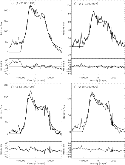 |
Figure 12:
The fits to the H
observed profiles for different
epochs, by an accretion disk model with an inclination angle of about
25,
and with a region of maximum emission at about 200 gravitation radius. The
dotted line represents the model profile, while the full thin line the observed
one. In each window, the lower panel represents the residuals for the following
dates:
 ,
2450701, 2451025, 2451426. ,
2450701, 2451025, 2451426. |
| Open with DEXTER | |
Using the virial theorem jointly with the reverberation-rms method
(cf. Peterson et al. 1998), the mass of the black hole in 3C 390.3
can be estimated from the relationship of Wandel et al. (1999):
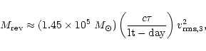 |
(4) |
 kms-1.
Using our results:
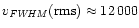 kms-1 (Fig.
  b),
b),
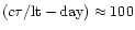 (Table
  ), we obtained
.
This value is substantially larger than
), we obtained
.
This value is substantially larger than
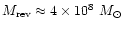 ,
obtained by Wandel et al. (1999). The difference is due to the fact
that the determination of Wandel et al. is based upon: 1) a time lag of 24 days,
instead of the 100-day lag found in the present study; 2) a value for
,
obtained by Wandel et al. (1999). The difference is due to the fact
that the determination of Wandel et al. is based upon: 1) a time lag of 24 days,
instead of the 100-day lag found in the present study; 2) a value for
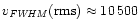 kms-1 instead of our value for
kms-1. The upper limit for the mass
of the BH in 3C 390.3, estimated from X-ray
variability is
kms-1 instead of our value for
kms-1. The upper limit for the mass
of the BH in 3C 390.3, estimated from X-ray
variability is
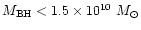 (Eracleous et al.
1997).
Assuming that
(Eracleous et al.
1997).
Assuming that
 ,
we estimate a value for
(the BH gravitational radius),
for the derived value of the BH mass:
,
we estimate a value for
(the BH gravitational radius),
for the derived value of the BH mass:
 cm.
cm.
According to our model calculations (Sect. 3.8), the bulk of Hemission is produced at
 ,
which corresponds to a time lag
,
which corresponds to a time lag
 light days.
This implies a shorter time lag than the one derived in this paper (Table
light days.
This implies a shorter time lag than the one derived in this paper (Table  ).
Can these values be reconciled?
The reverberation method assumes that the FWHM of the lines reflects virialized motions,
while we assumed that the motions are purely rotational.
These two working hypotheses may explain differences
in the size of the emitting region of the order of 40-50%. Then the time lag for
200
could be about
).
Can these values be reconciled?
The reverberation method assumes that the FWHM of the lines reflects virialized motions,
while we assumed that the motions are purely rotational.
These two working hypotheses may explain differences
in the size of the emitting region of the order of 40-50%. Then the time lag for
200
could be about
 lt.days. A value which is closer to
the mean lags listed in Table
lt.days. A value which is closer to
the mean lags listed in Table  :
:
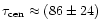 ;
and
;
and
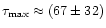 .
Worth mentioning is the good
agreement (within 20%) of the size of our disk, with that of a region (
.
Worth mentioning is the good
agreement (within 20%) of the size of our disk, with that of a region (
 )
containing
"cool dense material'' needed to reprocess X-ray radiation into the Fe Kalpha line, as
required by the observations of Eracleous et al.(1996).
)
containing
"cool dense material'' needed to reprocess X-ray radiation into the Fe Kalpha line, as
required by the observations of Eracleous et al.(1996).
The results of a 4-year (1995-1999) spectroscopic and
broad-band BVRI photometric monitoring of the AGN 3C 390.3 are
presented in this paper for the H
spectral region.
Our main conclusions are:
were observed.
and continuum fluxes vary by a factor
of about three during the time interval 1995-1999.
line
and the continuum,
with different durations were observed: (Fig.
 ): in (Oct. 1994-Jul. 1997) - a
brighter flare lasting 1000 days and another one in
(Jul. 1997-Jun. 1999) that lasted 700 days. The event duration is
defined as the interval between minima in the light curve.
): in (Oct. 1994-Jul. 1997) - a
brighter flare lasting 1000 days and another one in
(Jul. 1997-Jun. 1999) that lasted 700 days. The event duration is
defined as the interval between minima in the light curve.
100 days
in the response of the H
emission with respect to the
optical continuum changes is obtained from the observations at
any given time. Yet, for observations obtained between the June 1997
and 1999 (JD 2450618 - 2451527 - case C), a period in which the sampling
was better, a shorter lag of 33 to 36 days appears jointly with the one of 100 days. In light of
these results, we have to admit that either our data set is not
suitable for an accurate determination of the delays due to a
somewhat poor temporal sampling, or that the delay for 3C 390.3
varies with time, i.e. the correlation between the flux
variations in the continuum and in H
at different times
is not the same. In the 8 year monitoring campaign of NGC 5548,
Peterson et al. (1999) have determined that the time delay
had varied. They suggested that changes in the time
delays may be related to luminosity variations of the central source.
Yet, other investigation of NGC 5548 (Netzer & Maoz 1990) has
shown, that continuum variations with a long time scale - long-lasting flares - yield
longer time lags. Both posibilities are present in our
results for 3C 390.3 i.e.: a) the continuum outburst
of 1994-1997
with larger amplitude and duration (1000 days) yields a longer
time lag (100 days); b) the continuum outburst in 1997-1999 of a smaller
amplitude and duration (700 days) yields two lags: 100 and 35 days.
We believe that both the optical continuum and
flux variations
reflect
the changes in the X-ray irradiation, modulated by a variable accretion rate.
The radius of the
emission zone changes due to
surface temperature changes in the disk (Ulrich 2000).
 )
(i.e. whenever the flux
in the blue wing increases, that in the red wing also
increases). We have not detected a delay in the changes
of the H
blue wing (-7100 kms-1 to -1900 kms-1)
and of the red wing
(+1900 kms-1 to +7100 kms-1) with respect to the core of the
line
(-1900 kms-1 to +1900 kms-1) or relative to each other.
A similar
result was obtained by Dietrich et al. (1998) from monitoring
data for 3C 390.3 during 1994-1995. These results exclude the
presence of considerable radial motions in the BLR in
this object.
)
(i.e. whenever the flux
in the blue wing increases, that in the red wing also
increases). We have not detected a delay in the changes
of the H
blue wing (-7100 kms-1 to -1900 kms-1)
and of the red wing
(+1900 kms-1 to +7100 kms-1) with respect to the core of the
line
(-1900 kms-1 to +1900 kms-1) or relative to each other.
A similar
result was obtained by Dietrich et al. (1998) from monitoring
data for 3C 390.3 during 1994-1995. These results exclude the
presence of considerable radial motions in the BLR in
this object.
 d). The quasi-sinusoidal changes
(period 10 years) of the blue-to-red bump flux ratio
detected by Veilleux et al. (1991) are not present in our
data for the 1995-1999 lapse.
d). The quasi-sinusoidal changes
(period 10 years) of the blue-to-red bump flux ratio
detected by Veilleux et al. (1991) are not present in our
data for the 1995-1999 lapse.
profile has changed
drastically: during 1996, the blue and red bump emission was very strong,
while when the source was faintest (1997) the profiles had rather
flat tops (Fig.
 ). The blue wing was brighter than the red one
during the observed period.
). The blue wing was brighter than the red one
during the observed period.
narrow emission in 1995 until
Oct. 1999 follow the same trend found by Eracleous et al. (1997).
Their model for a binary BH with a very large mass value
(>10
)
seems to fit our data as well.
These authors argued that such a large value for the binary BH
mass is difficult to reconcile with other observations
and theory. Therefore, they reject the hypothesis of
a binary black hole for 3C 390.3. Our results provide further
support for the dismissal of the binary BH hypothesis for 3C 390.3,
on the basis of the masses required.
broad
emission revealed that the radial velocities of the blue and
red bumps in the profiles varied, showing an increase in
absolute value by about 2000 kms-1 during the observed period.
From these results (Table
 ,
Fig.
,
Fig.
 ),
it is infered that an annular zone in the accretion disk with enhanced Hemission could have moved towards smaller
radii between 1995 and 1999, i.e. larger Keplerian velocities as the flux in the continuum decreased (Table
),
it is infered that an annular zone in the accretion disk with enhanced Hemission could have moved towards smaller
radii between 1995 and 1999, i.e. larger Keplerian velocities as the flux in the continuum decreased (Table
 ).
These results are in agreement with a model in which the surface temperature
of the disk is modulated by the irradiation of a variable X-ray source (see Ulrich 2000 and references threin).
The X-ray variability on time scales of hours, days and
weeks is, in turn, modulated by accretion rate changes.
Thus, the peak velocity shifts, as different profiles
are also expected to result from the variable accretion rate
near the black hole.
).
These results are in agreement with a model in which the surface temperature
of the disk is modulated by the irradiation of a variable X-ray source (see Ulrich 2000 and references threin).
The X-ray variability on time scales of hours, days and
weeks is, in turn, modulated by accretion rate changes.
Thus, the peak velocity shifts, as different profiles
are also expected to result from the variable accretion rate
near the black hole.
line profiles in the
framework of an accretion disk model. We obtained a satisfactory
agreement for a disk with an inclination angle of about 25and with the region of maximum emission located at about 200 .
The radius of this zone is comparable to the one
in which the Fe Kalpha line emission originates, according to Eracleous et al.(1996).
.
The velocities of the blue and red bumps and their difference, obtained
from
difference profiles,
show a distinct anticorrelation with continuum flux changes.
Taking into consideration the time lag and the
flux,
we find that
the zone of maximal contribution to line emission moves across the face of
the disk.
It is located at smaller radii when the flux in the continuum decreases
(bump velocities increase), and to larger radii when the continuum flux
increases (bump velocities decrease).
These transient phenomena are expected to result
from the variable rate of accretion close to the black hole.
At low accretion rates, the flux from the central source may
decrease by a large factor, and the integral flux in the line could decrease.
Then, the maximum emission zone of the broad Balmer lines could shrink to such
small radii that the lines could become extremely broad and of low-contrast.
Consequently, at those times, they would be undetactable. This may be the
reason why the broad emission lines were not
seen in the 3C 390.3 spectrum in 1980 (Heckman et al. 1981)
or were
very weak in 1984 (Penston & Perez 1984). At those times the
central source brightness was in its long lasting minimum (Fig.  ).
).
It is interesting to note that the model calculations of Nicastro (2000)
point to a relationship between FWHM broad emission
lines and accretion rate for a given BH mass -
the lower the accretion rate, the greater the line width.
For different BH masses, there is a minimum value of the accretion
rate below which no broad lines are formed. The permitted interval of
velocities
ranges from 20000 kms-1 for sub-Eddington accretion rates
to 1000 kms-1 for Eddington accretion rates (i.e. the
lines with
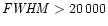 kms-1 do not exist for any mass of
the black hole).
kms-1 do not exist for any mass of
the black hole).
Acknowledgements
The authors want to thank M. Eracleous for providing some of the data used in Fig. 10. We would like to thank Didier Pelat for his help in the computation of the model profiles. We are grateful to G. M. Beskin for many useful discussions, to S. G. Sergeev for allowing us to use some of his software for spectral analysis tools, to O. Martinez for some spectral observations and to V. E. Zhdanova for help in data processing. This paper has had financial support from INTAS (grant N96-0328), RFBR (grant N97-02-17625, grant N00-02-16272a), scientific technical programme "Astronomy'' (Russia), RFBR+CHINE (grant 99-02-39120) and CONACYT research grants G28586-E, 28499-E and 32106-E (México).