A&A 376, 735-744 (2001)
DOI: 10.1051/0004-6361:20010984
New statistical goodness of fit techniques in noisy inhomogeneous
inverse problems
With application to the recovering of the luminosity distribution
of the Milky Way
N. Bissantz1 -
A. Munk2
1 - Astronomisches Institut der Universität Basel, Venusstr. 7, 4102 Binningen/Basel, Switzerland
2 - Fakultät für Mathematik und Informatik der Universität GH Paderborn,
Warburgerstr. 100, 33098 Paderborn, Germany
Received 16 June 2000 / Accepted 12 June 2001
Abstract
The assumption that a parametric class of functions fits the
data structure sufficiently well is common in
fitting curves and surfaces to regression data. One then derives
a parameter estimate resulting from a least squares fit, say, and
in a second step various kinds of  goodness of fit measures,
to assess whether the deviation between data and estimated surface is due to
random noise and not to systematic departures from the model.
In this paper we show that commonly-used -measures are invalid
in regression models, particularly when inhomogeneous noise is present.
Instead we present a bootstrap algorithm which is applicable in problems
described by noisy versions of Fredholm integral equations of the first kind.
We apply the suggested method to the problem of recovering
the luminosity density in the Milky Way from
data of the DIRBE experiment on board the
COBE satellite.
goodness of fit measures,
to assess whether the deviation between data and estimated surface is due to
random noise and not to systematic departures from the model.
In this paper we show that commonly-used -measures are invalid
in regression models, particularly when inhomogeneous noise is present.
Instead we present a bootstrap algorithm which is applicable in problems
described by noisy versions of Fredholm integral equations of the first kind.
We apply the suggested method to the problem of recovering
the luminosity density in the Milky Way from
data of the DIRBE experiment on board the
COBE satellite.
Key words: methods: data analysis - methods:
statistical - Galaxy: structure
Regression problems arise in almost any branch
of physics, including
astronomy and astrophysics. In general,
the problem of estimating a regression function (or surface)
occurs when a functional relationship between
several quantities of interest has to be
found from blurred observations (yi,ti),
 .
Here
.
Here
 denotes a vector of
measurements (response vector) and
denotes a vector of
measurements (response vector) and
 a quantity which affects the response vector in a
systematic but blurred way, which is to be investigated.
This systematic component is usually denoted
as the regression function
a quantity which affects the response vector in a
systematic but blurred way, which is to be investigated.
This systematic component is usually denoted
as the regression function
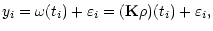
![$E[Y_i] = \omega(t_i)$](/articles/aa/full/2001/35/aa9993/img13.gif) .
Note that
Yi is a random variable, of which yi is a realisation.
If
.
Note that
Yi is a random variable, of which yi is a realisation.
If
 ,
this includes
signal detection problems or image restoration if
,
this includes
signal detection problems or image restoration if
 .
Many problems bear the additional difficulty that the quantity of interest
is not directly accesible to the observations y and
the relationship has to be expressed by a noisy
version of a Fredholm integral equation of the first
kind, viz.
.
Many problems bear the additional difficulty that the quantity of interest
is not directly accesible to the observations y and
the relationship has to be expressed by a noisy
version of a Fredholm integral equation of the first
kind, viz.
 |
|
|
(1) |
where  is a given integral operator,
  the
regression function to be reconstructed and
the
regression function to be reconstructed and
 a vector of independent
random quantities (error), due to imprecise measurements and other sources of
noise. More precisely, we assume that the expectation of yi is given by
a vector of independent
random quantities (error), due to imprecise measurements and other sources of
noise. More precisely, we assume that the expectation of yi is given by
 and inhomogeneous noise might be present, i.e.
the variance
and inhomogeneous noise might be present, i.e.
the variance
 of the noise
 (and possibly higher moments, too) depends on
the grid point ti.
There is a vast amount of literature concerning statistical theory for the
estimation of ,
we mention only Wand & Jones
(1995) for direct regression and
Nychka & Cox (1989) or van Rooij & Rymgaart
(1996) for the inverse (sometimes denoted as indirect)
case, as in Eq. (1).
(Inverse) regression models capture various examples from astronomy
and physics (cf. Bertero 1989 or Lucy
1994a, 1994b for an overview). Such an example is
the reconstruction
of the three-dimensional
luminosity in the Milky Way [MW], which will be discussed extensively
in Sect. 5. In this example,
will be a
three-dimensional density
of the MW,
the operator that projects this density to the sky,
(and possibly higher moments, too) depends on
the grid point ti.
There is a vast amount of literature concerning statistical theory for the
estimation of ,
we mention only Wand & Jones
(1995) for direct regression and
Nychka & Cox (1989) or van Rooij & Rymgaart
(1996) for the inverse (sometimes denoted as indirect)
case, as in Eq. (1).
(Inverse) regression models capture various examples from astronomy
and physics (cf. Bertero 1989 or Lucy
1994a, 1994b for an overview). Such an example is
the reconstruction
of the three-dimensional
luminosity in the Milky Way [MW], which will be discussed extensively
in Sect. 5. In this example,
will be a
three-dimensional density
of the MW,
the operator that projects this density to the sky,
 the resulting surface brightness at the sky position
ti=(l,b)i and yi the observed surface brightness at (l,b)i.
the resulting surface brightness at the sky position
ti=(l,b)i and yi the observed surface brightness at (l,b)i.
Reconstruction procedures (estimation) of
in general depend
on various a priori assumptions about ,
such as smoothness properties
or geometrical constraints, e.g. monotonicity.
The most common assumptions are that
has a particular structure and
shape, depending on some unknown parameter  .
Such an assumption is
denoted as a parametric model. Typically, these structural
assumptions arise from physical reasoning and approximation procedures.
Often, however, it is not completely clear whether
these assumptions are satisfied and therefore it is an important task
to investigate empirically (by means of the data at hand) whether the resulting model
is valid. Therefore, in this paper we discuss recent methodology
for the investigation of the adequacy of such a parametric model
.
Such an assumption is
denoted as a parametric model. Typically, these structural
assumptions arise from physical reasoning and approximation procedures.
Often, however, it is not completely clear whether
these assumptions are satisfied and therefore it is an important task
to investigate empirically (by means of the data at hand) whether the resulting model
is valid. Therefore, in this paper we discuss recent methodology
for the investigation of the adequacy of such a parametric model
 ,
,
 .
This will be done
for regular regression problems as well as for the inverse case, as in (1).
The paper is organized as follows.
In the next section we briefly review common practices to judge the
goodness of fit of a model U. It is shown that
classical goodness of fit approaches, such as least square statistics
are insufficient from many methodological points of view, particulary when
inhomogeneous noise is present, i.e. the variation
of the error
is expected to vary with the grid point (covariate) ti.
We show in Sect. 2 that statistically valid conclusions about the goodness of fit
from the residuals
.
This will be done
for regular regression problems as well as for the inverse case, as in (1).
The paper is organized as follows.
In the next section we briefly review common practices to judge the
goodness of fit of a model U. It is shown that
classical goodness of fit approaches, such as least square statistics
are insufficient from many methodological points of view, particulary when
inhomogeneous noise is present, i.e. the variation
of the error
is expected to vary with the grid point (covariate) ti.
We show in Sect. 2 that statistically valid conclusions about the goodness of fit
from the residuals
 (or variants of it) are impossible
in general, particularly when inhomogeneous noise is present, as is the case in
our data example. This is mainly due to the fact that in the inhomogeneous
case the distribution of
(or variants of it) are impossible
in general, particularly when inhomogeneous noise is present, as is the case in
our data example. This is mainly due to the fact that in the inhomogeneous
case the distribution of
 depends on the whole vector
 which is in general unknown.
Therefore, we suggest in Sect. 3 a measure of fit which is based on "smoothed residuals''
and which allows for the calculation of the corresponding probability distribution.
In Sect. 4, a bootstrap resampling algorithm
is suggested which allows the algorithmic reconstruction of the distribution
of the suggested goodness of fit quantity.
The use of bootstrap techniques is well documented in astronomy (cf. Barrow et al.
1984; Simpson & Mayer 1986; van den Bergh & Morbey
1984 for various applications). The work similar in spirit to ours
is Bi & Börner's (1994) residual type bootstrap, used as a method for
nonparametric estimation in inverse problems. As a byproduct we show, however, that
this residual bootstrap is insufficient in the case of inhomogeneous noise in the data
and a so-called "wild'' bootstrap has to be used instead.
which is in general unknown.
Therefore, we suggest in Sect. 3 a measure of fit which is based on "smoothed residuals''
and which allows for the calculation of the corresponding probability distribution.
In Sect. 4, a bootstrap resampling algorithm
is suggested which allows the algorithmic reconstruction of the distribution
of the suggested goodness of fit quantity.
The use of bootstrap techniques is well documented in astronomy (cf. Barrow et al.
1984; Simpson & Mayer 1986; van den Bergh & Morbey
1984 for various applications). The work similar in spirit to ours
is Bi & Börner's (1994) residual type bootstrap, used as a method for
nonparametric estimation in inverse problems. As a byproduct we show, however, that
this residual bootstrap is insufficient in the case of inhomogeneous noise in the data
and a so-called "wild'' bootstrap has to be used instead.
Finally we will apply our new method in Sect. 5 to the fit of the COBE/DIRBE L-band
data. We use a functional form for a parametric model of the MW as presented
by Binney et al. (1997, hereafter BGS) and find similar structural
parameters
of the Milky disk and bulge, except for the scale height of the disk which we find to
be about  smaller.
One of the most popular techniques for finding a
proper fit of a given model U to a given set of data
 is to
minimize a (penalized) weighted sum of squares
is to
minimize a (penalized) weighted sum of squares
where the
 denotes some weighting scheme and
the model is
denotes some weighting scheme and
the model is
 .
This leads to a weighted least squares
estimator (WLSE) of the optimal model parameter,
.
This leads to a weighted least squares
estimator (WLSE) of the optimal model parameter,
 .
However, it is well known that a proper choice of the weights
.
However, it is well known that a proper choice of the weights
 depends on the (possibly position-dependent)
random noise in the data. For example, under an uncorrelated normal error assumption,
if the variance
of the error
is assumed to be known, a suitable choice of weights is
depends on the (possibly position-dependent)
random noise in the data. For example, under an uncorrelated normal error assumption,
if the variance
of the error
is assumed to be known, a suitable choice of weights is
 in order to take into account the
local variability of the observations at the grid point ti.
Particularly, in this case, the ordinary, unweighted least squares estimator
is known to be insufficient (Gallant 1987), because the log likelihood
of the model is proportional to
in order to take into account the
local variability of the observations at the grid point ti.
Particularly, in this case, the ordinary, unweighted least squares estimator
is known to be insufficient (Gallant 1987), because the log likelihood
of the model is proportional to
 .
Only if the variance pattern is homogeneous (i.e.
.
Only if the variance pattern is homogeneous (i.e.
 )
are unweigthed least squares estimators optimal.
The weighted least squares approach is, however, limited if
the local variances
in the data points are unknown.
The
then have to be estimated from the data. This is often
neglected.
It is also common practice to consider Qnw in order to judge the
quality of fit achieved by the regression function (where the weights wi may
sometimes be different to those used in computing the WLSE).
Here, a "large'' value of Qnw is used as an indicator for a "significant'' deviation
between the observations and the model to be fitted. We will investigate this
in more detail in what follows, and emphasize the case of
nonhomogeneous variances.
)
are unweigthed least squares estimators optimal.
The weighted least squares approach is, however, limited if
the local variances
in the data points are unknown.
The
then have to be estimated from the data. This is often
neglected.
It is also common practice to consider Qnw in order to judge the
quality of fit achieved by the regression function (where the weights wi may
sometimes be different to those used in computing the WLSE).
Here, a "large'' value of Qnw is used as an indicator for a "significant'' deviation
between the observations and the model to be fitted. We will investigate this
in more detail in what follows, and emphasize the case of
nonhomogeneous variances.
In general, the most important properties required
of any goodness of fit (GoF) quantity
such as  are that
- 1)
- we are able to detect with high probability deviations from the model
we have in mind (often denoted by statisticians as good "power'');
- 2)
- we can quantify the probability that
exceeds some "critical value'' in order to obtain
a precise probabilistic analysis (computing significance levels, confidence intervals, etc.).
As a rough rule of thumb often
 |
|
|
(2) |
is taken as a measure of evidence for the model U and hence for the
fit of
 .
Here d
denotes the dimension (number of parameters) of U and n the number of
data points. Examples of the use of this kind of statistics can
be found in Alcock et al. (1997) and
in Dwek et al. (1995) in the context of discriminating between several models.
A related well-known quantity is the sum of squares of
"expected minus observed divided by expected''
for testing
distributional assumptions, such as normality of the data (cf. Cox & Hinkley 1974).
Bi & Börner (1994) considered a similar quantity
in a deconvolution setup which is, using the notation of (1)
.
Here d
denotes the dimension (number of parameters) of U and n the number of
data points. Examples of the use of this kind of statistics can
be found in Alcock et al. (1997) and
in Dwek et al. (1995) in the context of discriminating between several models.
A related well-known quantity is the sum of squares of
"expected minus observed divided by expected''
for testing
distributional assumptions, such as normality of the data (cf. Cox & Hinkley 1974).
Bi & Börner (1994) considered a similar quantity
in a deconvolution setup which is, using the notation of (1)
 |
|
|
(3) |
This obviously downweights the influence of residuals if the corresponding predicted value
 is large. Another option is to consider the absolute deviation of
the predicted and observed values, which leads to a more robust version of ,
or
even more general distance measures can be used (Cook & Weisberg 1999;
Hocking 1996; Lucy 1994a; 1994b).
In the following we will argue that an approach like
is large. Another option is to consider the absolute deviation of
the predicted and observed values, which leads to a more robust version of ,
or
even more general distance measures can be used (Cook & Weisberg 1999;
Hocking 1996; Lucy 1994a; 1994b).
In the following we will argue that an approach like  is not valid in regression
models such as (1), particularly when the noise is inhomogeneous or the
residuals are not gaussian. To this end we briefly discuss the (asymptotic)
distribution of the abovementioned quantities.
is not valid in regression
models such as (1), particularly when the noise is inhomogeneous or the
residuals are not gaussian. To this end we briefly discuss the (asymptotic)
distribution of the abovementioned quantities.
In order to get a first insight into the probabilistic behaviour of statistics such as
,
used as a quantitative measure of fit, it is helpful to consider
the distribution in the simplest case when
 .
A simple calculation then shows
that (assuming a normal distribution
of the data)
.
A simple calculation then shows
that (assuming a normal distribution
of the data)
 is distributed as a sum of normally distributed variables having the
expectation
is distributed as a sum of normally distributed variables having the
expectation
![$E[\chi^2] = \sum_{i=1}^{n}\sigma_i^2$](/articles/aa/full/2001/35/aa9993/img48.gif) ,
and variance
,
and variance
![$V[\chi^2] = 2\sum_{i=1}^{n}\sigma_i^4$](/articles/aa/full/2001/35/aa9993/img49.gif) .
Hence, already in this simple case it can be seen that the determination of the law of
is practically impossible if the variances
are
not known. Then it is difficult to quantify what a "too large value of
" means, because this will depend on the unknown quantities
.
Hence, already in this simple case it can be seen that the determination of the law of
is practically impossible if the variances
are
not known. Then it is difficult to quantify what a "too large value of
" means, because this will depend on the unknown quantities
 ,
and a rule as in (2) can lead in
principle to any result in favour or against the model
.
We mention that standardisation by the predicted values as in (3)
does not avoid this problem. This is in
contrast to goodness of fit problems
for the assessment of distribution assumptions, i.e.
when one investigates by a
measure whether
a population is normal, say (Cox & Hinkley 1974).
Note, that the case of homoscedastic regression models (i.e. the distribution of the
noise is identical for all data points) is somewhat simpler, because here the expectation
,
and a rule as in (2) can lead in
principle to any result in favour or against the model
.
We mention that standardisation by the predicted values as in (3)
does not avoid this problem. This is in
contrast to goodness of fit problems
for the assessment of distribution assumptions, i.e.
when one investigates by a
measure whether
a population is normal, say (Cox & Hinkley 1974).
Note, that the case of homoscedastic regression models (i.e. the distribution of the
noise is identical for all data points) is somewhat simpler, because here the expectation
![$E[\chi^2]=n\sigma^2$](/articles/aa/full/2001/35/aa9993/img51.gif) and the square root of the variance
and the square root of the variance
![$V[\chi^2]= 2n\sigma^4$](/articles/aa/full/2001/35/aa9993/img52.gif) is proportional, i.e. the signal to noise ratio
is proportional, i.e. the signal to noise ratio
![\begin{eqnarray*}\frac{E[\chi^2]}{\sqrt{V[\chi^2]}} = \sqrt{n/2}
\end{eqnarray*}](/articles/aa/full/2001/35/aa9993/img53.gif)
only depends on the number of data points n. Here, a model-free estimator of  can be used as a reference scale (Hart 1997).
Many attempts were
made in order to find simple approximations of the distribution for
.
Among them
a quite attractive option is use of a bootstrap method, an algorithmic
approximation of the true law (see Efron & Tibshirani 1993
for an overview and many applications).
Bootstrapping random quadratic forms (such as )
is, however, a rather delicate matter, because standard
bootstrap algorithms such as Efron's (1979) n out of n bootstrap are inconsistent
(Babu & Shankya 1984; Shao & Tu 1995), i.e. the distribution
is not approximated correctly with increasing number of observations.
The use of a particular bootstrap algorithm
was indeed suggested by Bi & Börner (1994) in the context
of assessing the goodness of fit
in deconvolution models. We mention that their bootstrap
algorithm, however, is asymptotically not correct
in inhomogeneous models.
Interestingly, the suggested algorithm is similar in
spirit to the so called residual bootstrap (i.e. drawing random samples with
replacement from the residuals ri) which is well documented
in the statistical literature (cf. Davison & Hinkley 1997, p. 281) for
the estimation of the regression parameters).
Despite the abovementioned difficulties,
the main problem encountered with the naive use of
in regression models as a measure of GoF is
that asymptotically (here and in the following, asymptotically means
the sample size tends to infinity) the law of
does in
general not converge asymptotically to any reasonable quantity, in contrast
to goodness of fit testing for distributional assumptions. Even after
rescaling by
 in order to force the variance
to converge (here it is assumed
that the scheme of grid points can be
described asymptotically by a distribution H (Dette & Munk 1998)) gives
which shows that
 does not converge to any reasonable quantity.
Note that if we use
does not converge to any reasonable quantity.
Note that if we use  the variance tends to zero.
Also observe that subtracting
the variance tends to zero.
Also observe that subtracting
![$E[1/ \sqrt n \; \chi^2]$](/articles/aa/full/2001/35/aa9993/img60.gif) from
will not provide a way out of the dilemma because this value depends
on the (unknown) variances
.
from
will not provide a way out of the dilemma because this value depends
on the (unknown) variances
.
In summary, we see that without explicit
knowledge of the variances
 ,
the use of
as a quantitative
measure of validity of a model is not appropriate.
,
the use of
as a quantitative
measure of validity of a model is not appropriate.
Due to the above-described difficulties, statisticians throughout the last two decades
have extensively studied the
problem of checking the goodness of fit in regression models.
It is beyond the scope of this paper to review
this work; many references can be found in the
recent monograph by Hart (1997). Among the variety of
procedures suggested so far, we mention methods
which are based on model selection criteria,
such as Akaike's (1974) information criterion
(Eubank & Hart 1992; Aerts et al. 1999)
and methods which compare nonparametric estimators with a parametric
estimator. To this end Azzalini & Bowman (1993),
Härdle & Mammen (1993)
and Müller (1992) used a kernel
estimator, Cox et al. (1988) smoothing splines and
Mohdeb & Mokkadem (1998) a Fourier series estimator.
However, the applicability of many of these methods is
often limited. For example, Härdle & Mammen's
test is confronted with bias problems, whereas
other procedures are only applicable for homogeneous
errors or when the error distribution is completely known
(Eubank & Hart 1992; Aerts et al. 1999).
Another serious difficulty arises with the nonparametric estimation of
the signal as the dimension k of the grid points increases. This
is sometimes denoted as the curse of dimensionality (Wand & Jones 1995;
Bowmann & Azzalini 1997).
A rough rule of thumb is that the number of observations required
in dimension k is nk in order to obtain the same
precision of the estimate of  .
Hence, the precision
induced by 100 observations on the real line is approximately the same as
10000 drawn from the plane. Furthermore,
measurements often cannot be taken equidistantly over a grid, which
leads to sparse data structures causing further difficulties
with increasing dimension.
One should also note that another difficulty consists of
transferring these methods to the case of inverse
problems, a situation which up to now has never been treated.
.
Hence, the precision
induced by 100 observations on the real line is approximately the same as
10000 drawn from the plane. Furthermore,
measurements often cannot be taken equidistantly over a grid, which
leads to sparse data structures causing further difficulties
with increasing dimension.
One should also note that another difficulty consists of
transferring these methods to the case of inverse
problems, a situation which up to now has never been treated.
Munk & Ruymgaart (1999)
have developed a general regression methodology which remains valid in
the heteroscedastic case (i.e. the distribution of the noise depends on
the data point) with arbitrary dimensions of the grid points. The
underlying idea dates back to H. Cramér and
can be summarized as "smoothing the residuals"
in order to obtain asymptotical stabilization of
the test criterion. In our context this reads
as follows. Let T denote an injective smoothing linear
integral operator with associated integral kernel
 ,
i.e.
,
i.e.
 = \int T(u, t) f(t) {\rm d}t.$](/articles/aa/full/2001/35/aa9993/img64.gif) |
|
|
(4) |
Note that since  is an integral operator,
![${\bf T}[f]$](/articles/aa/full/2001/35/aa9993/img66.gif) is again
a function. Now consider the transformed
distance between the parametric model
is again
a function. Now consider the transformed
distance between the parametric model
 and the distribution ,
which underlies the observations
and the distribution ,
which underlies the observations
 (cf. Sect. 1),
![$\displaystyle D^2 (g) = D^2({\bf T}[\omega]) = \min_{\vartheta \in \Theta}
\Vert {\bf T} [\omega-\omega_ {\vartheta}] \Vert^2$](/articles/aa/full/2001/35/aa9993/img69.gif) |
|
|
(5) |
where
![$g = {\bf T}[\omega]$](/articles/aa/full/2001/35/aa9993/img70.gif) denotes the smoothed version
of
and the norm
denotes the smoothed version
of
and the norm  refers to some
L2-norm to be specified later on.
The smoothed distance D2 serves now as a new measure
of goodness of fit and has to be estimated from data.
This will be done by numerical minimization of
the empirical counterpart of the r.h.s. of (5),
refers to some
L2-norm to be specified later on.
The smoothed distance D2 serves now as a new measure
of goodness of fit and has to be estimated from data.
This will be done by numerical minimization of
the empirical counterpart of the r.h.s. of (5),
 where
where
 denotes an estimator of g(u). In addition this provides
us with a smoothed estimator
denotes an estimator of g(u). In addition this provides
us with a smoothed estimator
 of the value
 for which the minimum
in (5) is achieved.
In Munk & Ruymgaart (1999)
the kernel
for which the minimum
in (5) is achieved.
In Munk & Ruymgaart (1999)
the kernel
was suggested (see Appendix A1), which will also be used in the following,
and which amounts to a cumulative smoothing.
Not that for
k-dimensional u and t the minimum has to be
understood componentwise as
We mention that other choices of T are possible (cf. Sect. A).
The reasoning behind this approach is that
direct estimation of
is a rather difficult
task, whereas estimation of the smoothed
transformation
 is much simpler.
Furthermore, the distribution of the minimizer of
is much simpler.
Furthermore, the distribution of the minimizer of
 becomes tractable.
If we denote the minimum of
becomes tractable.
If we denote the minimum of
 as
as  one can
show under very mild regularity conditions
that (Munk & Ruymgaart 1999) the distribution of
one can
show under very mild regularity conditions
that (Munk & Ruymgaart 1999) the distribution of
 converges to
 |
|
|
(6) |
where the  denotes a decreasing
sequence of positive numbers which depend on the best model parameter
denotes a decreasing
sequence of positive numbers which depend on the best model parameter
 ,
which is the minimizing
in (5),
the model space U and the unknown distribution
of the error
,
which is the minimizing
in (5),
the model space U and the unknown distribution
of the error
 ,
including the variance function
,
including the variance function
 .
This makes a
direct application of this limit law
difficult and hence a peculiar bootstrap algorithm
is suggested in the following which can be
shown to be asymptotically consistent, i.e.
the asymptotic limit law of this algorithm is the same as in
(6). The following idea of the so called
"wild bootstrap" dates back to Wu (1986) and
was applied by Stute et al. (1998) to a
testing problem similar to the one above.
.
This makes a
direct application of this limit law
difficult and hence a peculiar bootstrap algorithm
is suggested in the following which can be
shown to be asymptotically consistent, i.e.
the asymptotic limit law of this algorithm is the same as in
(6). The following idea of the so called
"wild bootstrap" dates back to Wu (1986) and
was applied by Stute et al. (1998) to a
testing problem similar to the one above.
4 The wild bootstrap algorithm
The true distribution (6) of
depends on the
unknown .
It is therefore not possible to use
this distribution for practical purposes.
However, it is possible to approximate the
distribution numerically using the following bootstrap
algorithm:
Step 1: (Generate residuals). Compute residuals
where
denotes a solution of the
minimization of
Step 2: (The "wild" part).
Generate new random variables
 ,
which do not depend on the data, where each
,
which do not depend on the data, where each
 is distributed to a distribution
which assigns probability
is distributed to a distribution
which assigns probability
 to the
value
to the
value
 and
and
 to the
value
to the
value
 .
See Fig. 1 for
a visualization of this probability distribution.
.
See Fig. 1 for
a visualization of this probability distribution.
Step 3: (Bootstrapping residuals). Compute
 and
and
 .
This gives a new data vector
.
This gives a new data vector
 .
.
Step 4: (Compute the target).
Compute
 with
.
with
.
Step 5: (Bootstrap replication). Repeat step 1-4 B
times (B=1000, say) which gives
values
 .
.
Now we construct the empirical cumulative distribution function [ECDF], which
can be taken as an approximation for the right side in (6), because
Munk & Ruymgaart (1999)
have shown that the ECDF, based on
 ,
asymptotically approximates the distribution
of .
The ECDF can be obtained by ordering the
values of
increasingly and plotting them
against the value (i)/B, where
(i) denotes the position of
in the ordered sample
,
asymptotically approximates the distribution
of .
The ECDF can be obtained by ordering the
values of
increasingly and plotting them
against the value (i)/B, where
(i) denotes the position of
in the ordered sample
 .
The so-called estimated
evidence of the model U can now be obtained by determining
the position of the original statistic
in the ordered sample
.
This
is some number
.
The so-called estimated
evidence of the model U can now be obtained by determining
the position of the original statistic
in the ordered sample
.
This
is some number
 .
From this number one computes
.
From this number one computes
Statisticians denote
 as the p-value of the test statistic .
The interpretation of this value is as follows. A small indicates that the observed data are very unlikely to have been
generated by model U, because the probability that
the observed (or a larger value)
occurs is very small,
namely
(recall that the bootstrap algorithm
reproduces the true distribution of
in (6)).
On the other hand, if
is large (and hence
small)
there should be
rare evidence against a proper use of model U, because
provides a good fit of the data to the model compared
to all other possible outcomes which could have occured.
as the p-value of the test statistic .
The interpretation of this value is as follows. A small indicates that the observed data are very unlikely to have been
generated by model U, because the probability that
the observed (or a larger value)
occurs is very small,
namely
(recall that the bootstrap algorithm
reproduces the true distribution of
in (6)).
On the other hand, if
is large (and hence
small)
there should be
rare evidence against a proper use of model U, because
provides a good fit of the data to the model compared
to all other possible outcomes which could have occured.
![\begin{figure}
\par\includegraphics[width=7.9cm,clip]{figure0.eps} \end{figure}](/articles/aa/full/2001/35/aa9993/Timg105.gif) |
Figure 1:
Binary probability distribution required in step 2
of the wild bootstrap algorithm. |
| Open with DEXTER |
A formal test at significance level
 can be performed
when deciding against U if
can be performed
when deciding against U if
 |
|
|
(7) |
In other words a small
 indicates that the deviation from the model U is not simply due to noise, but rather a
systematic devation from the model Uhas to be taken into account.
indicates that the deviation from the model U is not simply due to noise, but rather a
systematic devation from the model Uhas to be taken into account.
We would like to close this section by making some remarks
about the applicability of bootstrap algorithms in the
context of goodness of fit, and giving some arguments why
our bootstrap algorithm is valid in the heteroscedastic case.
Stute et al. (1998) have shown that the wild bootstrap is
valid in heteroskedastic models with
random grid points t.
This result can be extended to
deterministic grid points, as is the case in our example,
provided the scheme is not "too''
wiggly (a precise formulation can be found in
Munk 1999), which holds true for the subsequent example.
We mention that an explanation for the wild bootstrap validity
is its automatic adaptivity to inhomogeneous variances, because it
can be shown that the variance in the artifical datapoints
 induced by "wild'' resampling (step 2 in our algorithm) yields
which estimates approximately
.
In contrast, the n out
of n bootstrap (cf. Stute et al. 1998) and the residual bootstrap
here fail to hold because the bootstrap variance is in the latter
case
 ,
which approximates
the average overall variance
,
which approximates
the average overall variance
 in our example.
This argument transfers essentially to any random quadratic form
(such as
or Bi & Börner's 1994 -statistic).
The residual bootstrap is consistent
only if the error is homoscedastic, which, however,
in the subsequent example is not the case.
The case when the model space U is
of dimension
in our example.
This argument transfers essentially to any random quadratic form
(such as
or Bi & Börner's 1994 -statistic).
The residual bootstrap is consistent
only if the error is homoscedastic, which, however,
in the subsequent example is not the case.
The case when the model space U is
of dimension  ,
as
considered by Bi & Börner (1994), is in principle similar;
here it is also well known
that the residual bootstrap is insufficient in heteroscedastic models
(Härdle & Marron 1991).
,
as
considered by Bi & Börner (1994), is in principle similar;
here it is also well known
that the residual bootstrap is insufficient in heteroscedastic models
(Härdle & Marron 1991).
5 Application: Recovering the luminosity distribution in the Milky Way
The DIRBE experiment on board the COBE satellite,
launched in 1989,
made measurements of the surface brightness in several infrared wavebands
(Weiland 1994). A difficulty with the COBE/DIRBE
data is that it has to be corrected against certain effects.
The most important correction
is the removal of dust absorption. This has been done by Spergel et al. (1996).
We use their corrected COBE/DIRBE L-band data in our fits.
The resolution of the data are
 points
in l,b respectively, covering a range
points
in l,b respectively, covering a range
 and
and
 .
The points in this two-dimensional grid are equally spaced.
.
The points in this two-dimensional grid are equally spaced.
The COBE/DIRBE data have been used to deproject the three-dimensional density of the MW
in a number of projects. A main difficulty in
recovering the three-dimensional luminosity distribution from the two-dimensional
surface brightness distribution of the MW is that
it is not a unique operation, in general.
One way to avoid this problem is to fit a parametric model to the MW in
order to reduce the set of possible models.
Several parametric models have been suggested,
see for example Kent et al. (1991), Dwek et al. (1995) or Freudenreich (1998). Another approach is
to use the non-parametric Richardson-Lucy
algorithm for the deprojection of the data
(Binney & Gerhard 1996; Binney et al. 1997; Bissantz et al. 1997),
in order to reconstruct the luminosity distribution of the MW.
In parametric models of the MW density, about ten "structural
parameters'' - including normalisations, scale lengths and geometrical shape
parameters of the bulge/bar - are used (see, for example, Kent et al. 1991; Dwek et al. 1995;
Freudenreich 1998).
In what follows, we assume that these parameters are selected
such that the projection of a model onto the sky is an injective operation.
We will first derive a general
mathematical model of the problem of recovering the MW luminosity
distribution from the L-band data.
The projection of a three-dimensional light distribution
to a surface brightness (on the sky) is defined as follows.
Let  be the set of possible luminosity densities of the MW, i.e.
of maps
be the set of possible luminosity densities of the MW, i.e.
of maps
and  be the surface brightness distributions
where
 is the surface brightness at sky position (l,b),
and
is the surface brightness at sky position (l,b),
and
 .
The transformation between
a luminosity density
to its corresponding
surface brightness distribution
is described by
a linear integral operator
.
The transformation between
a luminosity density
to its corresponding
surface brightness distribution
is described by
a linear integral operator  .
We will call this operator
the projection operator, since it "projects'' a luminosity
density on the sky, i.e. onto a surface brightness distribution.
.
We will call this operator
the projection operator, since it "projects'' a luminosity
density on the sky, i.e. onto a surface brightness distribution.
is defined by the integral
 of the density
 along the line-of-sight from the observer to infinity in
direction (l,b). Let r denote the distance from the
observer. Note that the integrand is
and not
along the line-of-sight from the observer to infinity in
direction (l,b). Let r denote the distance from the
observer. Note that the integrand is
and not
 because the physical extend of the observed cone
 increases as r2 whereas
the intensity of a source decreases as r-2 and the r-powers
therefore cancel out.
Let
increases as r2 whereas
the intensity of a source decreases as r-2 and the r-powers
therefore cancel out.
Let
 be the path from the observer to infinity
along the line-of-sight to (l,b), parametrized by
the distance from the observer r. Then
be the path from the observer to infinity
along the line-of-sight to (l,b), parametrized by
the distance from the observer r. Then
So far we have used a spherical coordinate system centered at the observer.
Coordinate axes are the sky longitude l and latitude b and the
distance from the observer r.
We now introduce a second coordinate system.
Let (x,y,z) be the coordinate axes of a cartesian, galactocentric,
coordinate system, s.t. x and y lie in the main plane of the MW. We define
x to be along the major axis of the bulge/bar (cf. Sect. 5.2 for
further explanation of the components of our parametric MW model, including
the bulge/bar), y along the minor axis, and z
perpendicular to the main plane of the MW.
Let us further call "bar angle  '' the angle between the major axis
of the bar/bulge and the line-of-sight direction from the observer to the
galactic centre. The position of the observer in this coordinate system is
denoted as
'' the angle between the major axis
of the bar/bulge and the line-of-sight direction from the observer to the
galactic centre. The position of the observer in this coordinate system is
denoted as
 .
Figure 2 depicts the two coordinate systems.
.
Figure 2 depicts the two coordinate systems.
![\begin{figure}
\par\includegraphics[width=6.7cm,clip]{coo.eps} \end{figure}](/articles/aa/full/2001/35/aa9993/Timg132.gif) |
Figure 2:
A sketch of the two coordinate systems that we use in this
paper. Luminosity densities of the MW are defined in the galactocentric
coordinate system x,y,z. Galactic longitude l and latitude bdefine a position on the sky. Together with the distance from the observer r they constitute the observer centered coordinate system. |
| Open with DEXTER |
In our setting, a parametric model of the
MW is a class U of distributions
 such that
where  denotes a
set of parameters
denotes a
set of parameters
 .
This definition is
in accordance with our terminology at the beginning of this paper.
We cannot observe
directly, due to measurement errors,
dust removal from the raw data and other sources of noise.
Hence, our observations
.
This definition is
in accordance with our terminology at the beginning of this paper.
We cannot observe
directly, due to measurement errors,
dust removal from the raw data and other sources of noise.
Hence, our observations
 are blurred by some random error
 ,
the distribution
of which may vary between different sky positions
(li, bj).
Particularly, we will see in the following that it is necessary to
allow for a position-dependent noise
,
the distribution
of which may vary between different sky positions
(li, bj).
Particularly, we will see in the following that it is necessary to
allow for a position-dependent noise
![$Var[\varepsilon_{i,j}]=\sigma^2_{i,j}$](/articles/aa/full/2001/35/aa9993/img139.gif) .
Therefore our astrophysical problem is
to reconstruct
from the noisy integral equation.
.
Therefore our astrophysical problem is
to reconstruct
from the noisy integral equation.
Note that this is a noisy Fredholm equation of the first kind as
in (4);
the suggested method in the last section
transfers directly to the present setting.
Note, that
is a linear injective operator as long as
 due to our selection of the parametric model.
Let
and consider the transformed model
where
and
Specific models U will be discussed in the next section
Following the approach in
Sect. 4 we specify the smoothing
integral operator T by defining the smoothing kernel as
This amounts to a kind of cumulative smoothing, which downweights small-scale
features in the data, and emphasizes trends on large scales.
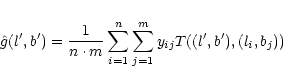
Now, as a first step, we estimate
$](/articles/aa/full/2001/35/aa9993/img147.gif) by
by
and determine numerically the "transformed'' LSE
![$\displaystyle \hat{\vartheta}_{\bf T}
= \textrm{argmin}_{\vartheta\in\Theta} \vert\vert\hat{g}-{\bf T}[\omega_{\vartheta}]\vert\vert^2$](/articles/aa/full/2001/35/aa9993/img149.gif) |
|
|
(8) |
where
 denotes the usual L2-norm.
Finally, the minimising value
denotes the usual L2-norm.
Finally, the minimising value
is computed. Now the bootstrap algorithm in Sect. 4
can be applied.
Finally, we mention that for the minimization in (8)
we have used the Marquardt-Levenberg algorithm (Press et al. 1994).
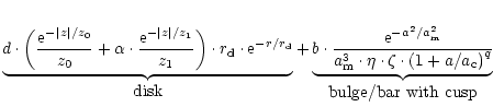
5.2 A parametric model of the Milky Way
We will now investigate
whether the functional form of the luminosity distribution
of the MW as suggested by BGS
provides a satisfactory fit to the COBE/DIRBE L-band data.
This functional form is a superposition of a double-exponential disk with a truncated
power-law bulge
where the parameter
can be devided into "structural'' parameters
 that specify
the functional form of the model and "geometrical'' parameters that
define the position of the sun in the coordinate system.
The "geometrical'' parameters are fixed in advance and are the position
of the sun above the main plane of the MW,
that specify
the functional form of the model and "geometrical'' parameters that
define the position of the sun in the coordinate system.
The "geometrical'' parameters are fixed in advance and are the position
of the sun above the main plane of the MW,
 pc, the distance of the sun from the galactic centre projected
on the main plane,
pc, the distance of the sun from the galactic centre projected
on the main plane,
 kpc and the bar angle,
 (BGS). It is not feasible
to estimate the cusp parameters
(BGS). It is not feasible
to estimate the cusp parameters
 pc and q=1.8
from our data, because the available resolution is not sufficient. We use
the same values as BGS.
pc and q=1.8
from our data, because the available resolution is not sufficient. We use
the same values as BGS.
As a first step we will investigate graphically
whether an inhomogeneous variance pattern has to be assumed,
which is indicated by inhomogeneous squares of residuals.
Figure 3 shows the COBE/DIRBE L-band data and Fig. 4 the residuals
 ,
with the
model parameters
,
with the
model parameters
 taken from BGS.
Provided this model holds (approximately)
true, as an important conclusion from Fig. 4 we find
strong indication for inhomogeneous noise. Interestingly, towards the boundary
of the observed part of the sky, the variability of the observations increases.
Figure 6 shows the difference between the
model and the data including the algebraic sign of the difference. Note that
the error distribution is obviously inhomogeneous, both in the logarithmic
magnitude scale plotted in the figures and in a linear scale.
Further note there is a systematic dependence of the sign of the deviations
on the position on the sky, whereas the model fits well in the central part
of the observed part of the sky.
This is indication that the MW disk shows deviations from an exponential
taken from BGS.
Provided this model holds (approximately)
true, as an important conclusion from Fig. 4 we find
strong indication for inhomogeneous noise. Interestingly, towards the boundary
of the observed part of the sky, the variability of the observations increases.
Figure 6 shows the difference between the
model and the data including the algebraic sign of the difference. Note that
the error distribution is obviously inhomogeneous, both in the logarithmic
magnitude scale plotted in the figures and in a linear scale.
Further note there is a systematic dependence of the sign of the deviations
on the position on the sky, whereas the model fits well in the central part
of the observed part of the sky.
This is indication that the MW disk shows deviations from an exponential
 -dependence.
![\begin{figure}
\par\includegraphics[width=13.5cm,clip]{9993f3.eps} \end{figure}](/articles/aa/full/2001/35/aa9993/Timg164.gif) |
Figure 3:
COBE/DIRBE L-band data. Contours levels are given in
magnitudes. Note that contour levels are only defined up to a common
offset. |
| Open with DEXTER |
![\begin{figure}
\par\includegraphics[width=13.09cm,clip]{9993f4.eps} \end{figure}](/articles/aa/full/2001/35/aa9993/Timg166.gif) |
Figure 4:
Square difference between COBE/DIRBE L-band data logarithmic
surface brightness (magnitudes) and the parametric model with the
parameters from BGS.
Contours levels are
 . . |
| Open with DEXTER |
![\begin{figure}
\par\includegraphics[width=13.2cm,clip]{9993f5.eps} \end{figure}](/articles/aa/full/2001/35/aa9993/Timg167.gif) |
Figure 5:
The smoothed COBE/DIRBE L-band data. This is the observed
data in the sky region
 and
and
 ,
after application of the smoothing operator T. Contours indicated are for
the natural logarithm of ,
after application of the smoothing operator T. Contours indicated are for
the natural logarithm of
 .
Note
that the x and y axis are from
and
,
due to the definition of T. .
Note
that the x and y axis are from
and
,
due to the definition of T. |
| Open with DEXTER |
We now determine the best-fit model parameter
 by
minimisation of .
We use the parameters found by BGS as starting values
for our minimisation algorithm.
Due to the increasing noise towards the boundary of the observed part of the sky,
we restrict the region of the surface brightness data used in the fit
to the region
by
minimisation of .
We use the parameters found by BGS as starting values
for our minimisation algorithm.
Due to the increasing noise towards the boundary of the observed part of the sky,
we restrict the region of the surface brightness data used in the fit
to the region
 and
and
 .
This is done to downweight those parts of the
sky where noninformative parts in the data are expected (see Fig. 4).
Figure 5 shows this data after it has been smoothed with
the smoothing operator .
Note how much smoother the smoothed data appears
compared to the original COBE/DIRBE L-band data.
Our computational strategy consists of two steps.
.
This is done to downweight those parts of the
sky where noninformative parts in the data are expected (see Fig. 4).
Figure 5 shows this data after it has been smoothed with
the smoothing operator .
Note how much smoother the smoothed data appears
compared to the original COBE/DIRBE L-band data.
Our computational strategy consists of two steps.
- 1. Fitting the disk: in the first step we fit the disk parameters with fixed bulge parameters;
- 2. Fitting the bulge/bar: in the second step we fix
the disk related parameters found in the first step (except for the
normalisation parameter d)
and fit the bulge/bar parameters and d.
Table 1 shows our result for the best-fit model parameters
 and the model parameters of BGS. As suggested in Sect. 4 we have obtained our best-fit model parameters by minimisation of .
Note that BGS have not used exactly the same region of the sky in their fit
as we use here. Therefore, one has to take into account that differences between
these model parameters may be partially due to different
regions of the sky (data) used in the fit. We reduce this problem by redetermining
the normalisations b,d of the model by BGS (keeping fixed their other parameters)
with our algorithm, using the region of the sky selected above.
The value of our proposed statistical quantity
for the
BGS model has been calculated for this modified version of their model parameters.
and the model parameters of BGS. As suggested in Sect. 4 we have obtained our best-fit model parameters by minimisation of .
Note that BGS have not used exactly the same region of the sky in their fit
as we use here. Therefore, one has to take into account that differences between
these model parameters may be partially due to different
regions of the sky (data) used in the fit. We reduce this problem by redetermining
the normalisations b,d of the model by BGS (keeping fixed their other parameters)
with our algorithm, using the region of the sky selected above.
The value of our proposed statistical quantity
for the
BGS model has been calculated for this modified version of their model parameters.
![\begin{figure}
\par\includegraphics[width=13.2cm,clip]{9993f6.eps} \end{figure}](/articles/aa/full/2001/35/aa9993/Timg176.gif) |
Figure 6:
Difference between COBE/DIRBE L-band data logarithmic
surface brightness (magnitudes) and the parametric model
from BGS in magnitudes. Negatives values for the contour
levels indicate that a model is too bright as compared to the data. The contour
levels are chosen such that their squares are equivalent to  0.1 mag2,
0.2 mag 0.1 mag2,
0.2 mag
 0.3 mag2, to allow a direct comparison with
Fig. 4. 0.3 mag2, to allow a direct comparison with
Fig. 4. |
| Open with DEXTER |
Applying the bootstrap algorithm presented in Sect. 4 to
our model we
find that
 ,
which indicates
no significant evidence against this model.
For the parameters found in BGS
a value
,
which indicates
no significant evidence against this model.
For the parameters found in BGS
a value
 is obtained which yields a slightly worse
fit. Note that, at a first glance,
this statement is in contradiction to the argument
given by BGS in the last paragraph of their p. 366. They pointed
out that a graphical inspection of residuals
suggests that for the model considered,
some local regions of the sky seem to
show systematic differences between their model and the observed data.
As a conclusion we find that the proposed
method is not capable of concluding
that these local deviations between model and data are due
to systematic deviations.
As pointed out by the referee this might be due to
lack of power of the proposed method,
because an additional smoothing step was proposed.
Indeed, this corresponds to some theoretical results
concerning the asymptotic efficiency of the proposed method
(Munk & Ruymgaart 1999).
In fact, a more powerful method
could result from chosing a data-driven smoothing operator ,
similar
to bandwidth selection in kernel regression.
The main difficulty which arises is a different
limit law compared to the case discussed
in the present, where
is fixed.
However, this is beyond the scope
of this paper and will be an interesting topic for further research.
is obtained which yields a slightly worse
fit. Note that, at a first glance,
this statement is in contradiction to the argument
given by BGS in the last paragraph of their p. 366. They pointed
out that a graphical inspection of residuals
suggests that for the model considered,
some local regions of the sky seem to
show systematic differences between their model and the observed data.
As a conclusion we find that the proposed
method is not capable of concluding
that these local deviations between model and data are due
to systematic deviations.
As pointed out by the referee this might be due to
lack of power of the proposed method,
because an additional smoothing step was proposed.
Indeed, this corresponds to some theoretical results
concerning the asymptotic efficiency of the proposed method
(Munk & Ruymgaart 1999).
In fact, a more powerful method
could result from chosing a data-driven smoothing operator ,
similar
to bandwidth selection in kernel regression.
The main difficulty which arises is a different
limit law compared to the case discussed
in the present, where
is fixed.
However, this is beyond the scope
of this paper and will be an interesting topic for further research.
It can be seen from Table 1 that the main difference between the
two models is that our model has a lower disk scale height z0.
The value
was found to be slightly better for our new model compared to
the BGS parameters. However, recall that
we used only a part of the COBE/DIRBE L-band surface brightness
data in our fit.
We have
argued that classical measures of goodness of fit adopted from
checking distributional assumptions
can be misleading in the context of (inverse) regression.
Particularly, an inhomogeneous noise field can
inflate the precision of common
quantities.
For this case, a new method was proposed for noisy Fredholm equations of the first kind
by Munk & Ruymgaart (1999). As an example for the application of the
suggested algorithm, we use the problem of determining the luminosity density in the
MW from surface brightness data. From this we have found that the parametric model in
Binney et al. (1997) can be improved slightly and gives
a satisfactory fit of the COBE/DIRBE L-band data in a range of
.
Acknowledgements
The authors are indebted to the organizers F. Ruymgaart,
W. Stute and Y. Vardi of the conference
"Statistics for Inverse Problems'' held
at the Mathematical Research Center at Oberwolfach, Germany, 1999.
The present paper was essentially initiated by this meeting.
We would like to thank O. Gerhard and the referee, P. Saha, for
many helpful comments. N. Bissantz acknowledges support by
the Swiss Science Foundation under grant number 20-56888.99.
Appendix A: Chosing the smoothing kernel T
We mention that our procedure can also be performed with any other
smoothing kernel T. This will also yield
in general different values of .
In principle, a valid option is any
injective Operator .
A good choice of ,
however,
is driven by various aspects, such as efficiency or simplicity.
An extensive simulation study performed in Munk & Ruymgaart (1999),
reveals the kernel
 as a reasonable choice which
yields a procedure capable to detect a broad range of deviations from
U. See, however, the discussion in Sect. 5.
A particularly simple choice in noisy inverse models
as a reasonable choice which
yields a procedure capable to detect a broad range of deviations from
U. See, however, the discussion in Sect. 5.
A particularly simple choice in noisy inverse models
can be achieved if
T is the adjoint of
K itself, provided
K is a smoothing operator of the type
However, in our application this is not easy to calculate and
will depend on constraints which force the particular model
to be identifiable.
-
Aerts, M., Claeskens, G., & Hart, J. 1999, J. Amer. Statist. Assoc., 94, 869
In the text
-
Akaike, H. 1974, IEEE Trans. Autom. Control, 19, 716
In the text
-
Alcock, C., Allsman, R. A., Alves, D., et al. 1997, ApJ, 486, 697
In the text
NASA ADS
-
Azzalini, A., & Bowman, A. W. 1993, Jour. Roy. Statist. Soc. Ser. B, 55, 549
In the text
-
Babu, G. J. 1984, Shankya A, 46, 85
In the text
-
Barrow, J. D., Sonoda, D. H., & Bhavsar, S. P. 1984, MNRAS, 210, 19
In the text
-
van den Bergh, S., & Morbey, C. L. 1984, ApJ, 283, 598
In the text
NASA ADS
-
Bertero, M. 1989, Adv. Electron. El. Phys., 75, 1
In the text
-
Bi, H., & Boerner, G. 1994, A&AS, 108, 409
In the text
NASA ADS
-
Binney, J., & Gerhard, O. 1996, MNRAS, 279, 1005
In the text
NASA ADS
-
Binney, J., Gerhard, O., & Spergel, D. 1997, MNRAS, 288, 365 (BGS)
In the text
NASA ADS
-
Bissantz, N., Englmaier, P., Binney, J., et al. 1997, MNRAS, 289, 651
In the text
NASA ADS
-
Bowman, A. W.,
& Azzalini, A. 1997,
Applied smoothing
techniques for data
analysis: the kernel
approach with S-Plus
illustrations, Oxford Statistical
Science Series (Oxford:
Oxford University Press), 18
In the text
-
Cook, R. D., & Weisberg, S. 1999,
Applied Regression Including Computing and Graphics
(New York, NY: Wiley)
In the text
-
Cox, D. R., & Hinkley, D. V. 1974,
Problems and solutions in theoretical statistics
(A Halsted Press Book, London: Chapman and Hall; New York: John Wiley & Sons)
In the text
-
Cox, D., Koh, E., Wahba, G., & Yandell, B. S. 1988,
Ann. Statist., 18, 113
In the text
-
Davison, A. C., & Hinkley, D. V. 1997,
Bootstrap methods and their application,
Cambridge Series on Statistical and Probabilistic Mathematics (Cambridge: Cambridge University Press)
In the text
-
Dette, H., & Munk, A. 1998, Ann. Stat., 26, 778
In the text
-
Dwek, E., Arendt, R. G., Hauser, M. G., et al. 1995, ApJ, 445, 716
In the text
NASA ADS
-
Efron, B. 1979, Ann. Stat., 7, 1
In the text
-
Efron, B., & Tibshirani, R. J. 1993,
An Introduction to the Bootstrap,
Monographs on Statistics and Applied Probability (New York, NY: Chapman & Hall), 57
In the text
-
Eubank, R. L., & Hart, J. D. 1992, Ann. Stat., 20, 1412
In the text
-
Freudenreich, H. T. 1998, ApJ, 492, 495
In the text
NASA ADS
-
Gallant, A. R. 1987, Nonlinear Statistical Models,
Wiley Series in Prob. & Math. Stat. (Wiley: New York)
In the text
-
Härdle, W., & Mammen, E. 1993, Ann. Stat., 21, 1926
In the text
-
Härdle, W., & Marron, J. S. 1991,
Ann. Stat., 19, 778
In the text
-
Hart, J. D. 1997, Nonparametric smoothing and lack of fit tests,
Springer Series in Statistics (Springer)
In the text
-
Hocking, R. R. 1996,
Methods and Applications of Linear Models
(New York, NY: Wiley)
In the text
-
Kent, S. M., Dame, T. M., & Fazio, G. 1991, ApJ, 378, 131
In the text
NASA ADS
-
Lucy, L. B. 1994a, A&A, 289, 983
In the text
NASA ADS
-
Lucy, L. B. 1994b, Rev. Mod. Astron., 7, 31
In the text
NASA ADS
-
Mair, B. A., & Ruymgaart, F. H. 1997, SIAM J. Appl. Math., 56, 1424
-
Matthai, A. M., & Provost, S. B. 1992, Quadratic forms in Random Variables
(Marcel Dekker, NY)
-
Mohdeb, Z., & Mokkadem, A. 1998,
C. R. Acad. Sci., Paris, Ser. I, Math., 326(9), 1141
In the text
-
Müller, H. G. 1992, Scand. J. Stat., 19, 157
In the text
-
Munk, A. 1999, under revision, Scand. J. Stat.
In the text
-
Munk, A., & Ruymgaart, F. 1999, submitted
-
Nychka, D. W., & Cox, D. D. 1989,
Ann. Stat., 17, 556
In the text
-
Press, W. H., Teukolsky, S. A., Vetterling, W. T., et al. 1994, Numerical recipes in C, 2nd Ed.
(Cambridge: Cambridge University Press)
In the text
-
van Rooij, & Ruymgaart, F. H. 1996, J. Stat. Plann.
Infer., 53, 389
In the text
-
Shao, J., & Tu, D. 1995, The Jacknife and Bootstrap
(Springer, NY)
In the text
-
Shorack, G., & Wellner, J. 1986, Empirical Process with Applications to
Statistics (Wiley, NY)
-
Simpson, G., & Mayer-Hasselwander, H. 1986, A&A, 162, 340
In the text
NASA ADS
-
Spergel, D. N., Malhotra, S., & Blitz, L. 1995,
Towards a Three-Dimensional Model of the Galaxy, in
ESO/MPA Workshop on Spiral Galaxies in
the Near-I, ed. D. Minniti, & H.-W. Rix (Springer), 1996
In the text
- Stute, W., Gonzáles-Manteiga, W.,
& Presedo Quindimil, M.
1998, J. Amer. Stat. Assoc., 93, 141
In the text
-
Wand, M. P., & Jones, M. C. 1995, Kernel smoothing,
Monographs on Statistics and
Applied Probability
(London: Chapman & Hall), 60
In the text
-
Weiland, J. L., et al. 1994,
ApJ, 425, L81
In the text
NASA ADS
-
Wu, C. F. J. 1986, Ann. Stat., 14, 1261
In the text
Copyright ESO 2001
![\begin{eqnarray*}V\left[1/ \sqrt n \; \chi^2\right] = 2/n \sum_{i=1}^{n}\sigma_i...
...row \infty}{\longrightarrow} \;
2 \int \sigma^4 (t) H({\rm d}t)
\end{eqnarray*}](/articles/aa/full/2001/35/aa9993/img56.gif)
![\begin{eqnarray*}E\left[1/ \sqrt n \; \chi^2\right] = \sqrt n \left( 1/n \sum_{i=1}^{n}\sigma_i^2\right)
\, = O(\sqrt{n}) \, \rightarrow
\infty
\end{eqnarray*}](/articles/aa/full/2001/35/aa9993/img57.gif)

![\begin{eqnarray*}V^{\ast}[\varepsilon^{\ast}_i] = \hat\varepsilon_i^2
\end{eqnarray*}](/articles/aa/full/2001/35/aa9993/img109.gif)
![\begin{eqnarray*}\omega: \left[0,2\pi\right]\times\left[-\frac{\pi}{2},\frac{\pi...
...
\rightarrow {\rm I\!R}_{\geq 0},
(l,b) \mapsto \omega (l,b),
\end{eqnarray*}](/articles/aa/full/2001/35/aa9993/img119.gif)
![\begin{figure}
\par\includegraphics[width=6.7cm,clip]{coo.eps} \end{figure}](/articles/aa/full/2001/35/aa9993/img132.gif)
 = \int\int \omega(l,b) T((l',b'), (l,b)) {\rm d}l{\rm d}b.
\end{eqnarray*}](/articles/aa/full/2001/35/aa9993/img145.gif)
![\begin{eqnarray*}\hat{D}^2= \vert\vert\hat{g}-{\bf T}[{\cal P}\left(\rho_{\hat{\vartheta}_{\bf T}}\right)]\vert\vert^2
\end{eqnarray*}](/articles/aa/full/2001/35/aa9993/img151.gif)