A&A 376, 381-385 (2001)
DOI: 10.1051/0004-6361:20011005
Cosmic background of gravitational waves from rotating neutron stars
T. Regimbau - J. A. de Freitas Pacheco
Observatoire de la Côte d'Azur, BP 4229, 06304 Nice Cedex 4, France
Received 25 April 2001 / Accepted 10 May 2001
Abstract
The extragalactic background of gravitational waves produced
by tri-axial rotating neutron stars was calculated, under the assumption
that the properties of the underlying pulsar population are the same of
those of the galactic population, recently derived by Regimbau & de Freitas
Pacheco (2000). For an equatorial ellipticity of
 = 10-6,
the equivalent density parameter due to gravitational
waves has a maximum amplitude in the range
2
= 10-6,
the equivalent density parameter due to gravitational
waves has a maximum amplitude in the range
2 10
10
 10-9, around
0.9-1.5 kHz. The main factors affecting the theoretical predictions are
discussed. This
background is comparable to that produced by the "ring-down'' emission from
distorted black holes. The detection possibility of this background by a future
generation of gravitational antennas is also examined.
10-9, around
0.9-1.5 kHz. The main factors affecting the theoretical predictions are
discussed. This
background is comparable to that produced by the "ring-down'' emission from
distorted black holes. The detection possibility of this background by a future
generation of gravitational antennas is also examined.
Key words: pulsars: general - gravitational waves - stars: neutron
In the past years, a large number of papers devoted to stochastic
backgrounds of gravitational waves appeared in the literature (see
Maggiore 2000 for a recent review). Besides processes that took place
very shortly after the big-bang, the emission from a large number
of unresolved sources can produce a stochastic background. Supernovas
(Blair et al. 1997) and distorted black holes (Ferrari et al. 1999a;
de Araújo et al. 2000) are examples of sources able to generate shot
noise, while a truly continuous background could
be produced, for instance, by the "r-mode'' emission from young and
hot neutron stars (Owen et al. 1998; Ferrari et al. 1999b).
Detection of such backgrounds may probe the cosmic star
formation rate up to redshifts of
 ,
the mass range of the progenitors of neutron stars and black holes as well as
the initial angular momentum of these objects.
,
the mass range of the progenitors of neutron stars and black holes as well as
the initial angular momentum of these objects.
The contribution of the entire population of rotating neutron stars to the
continuous
galactic background of gravitational waves was considered by different authors
(Schutz 1991; Giazotto et al. 1997; de Freitas Pacheco & Horvath
1997)
and, more
recently, this subject was revisited by Regimbau & de Freitas Pacheco (2000, hereafter
RP00). In the latter, the "true'' population of rotating neutron stars
was synthesized by
Monte Carlo techniques and its contribution to the galactic background
of gravitational waves
was estimated. If the planned sensitivity of the first generation of laser
beam interferometers
is taken into account (in particular that of the French-Italian
project VIRGO), then the
simulations by RP00 suggest that only few objects will contribute to the
signal, if the
mean equatorial ellipticity of neutron stars is of the order
of
= 10-6.
Upper limits on
have been obtained by assuming that the
observed spin-down
of pulsars is essentially due to the emission of gravitational waves. In
this case, one obtains
 10-3 for "normal'' pulsars whereas recycled or
rejuvenated
pulsars seem to have equatorial deformations less than 10-8.
Although the galactic population will not produce a real background, the
integrated contribution of these objects remains to be investigated
in a large volume of the universe. Estimates of this emission are important
because it may rival with the background of possible cosmological
origin. Since there is an upper limit to the wave frequency of the
pulsar gravitational
radiation, a putative cosmic background will dominate at low frequencies
and the knowledge of the spectral energy distribution of the background
produced by discrete sources may help in the choice of the best frequency
domain to search for a relic emission.
10-3 for "normal'' pulsars whereas recycled or
rejuvenated
pulsars seem to have equatorial deformations less than 10-8.
Although the galactic population will not produce a real background, the
integrated contribution of these objects remains to be investigated
in a large volume of the universe. Estimates of this emission are important
because it may rival with the background of possible cosmological
origin. Since there is an upper limit to the wave frequency of the
pulsar gravitational
radiation, a putative cosmic background will dominate at low frequencies
and the knowledge of the spectral energy distribution of the background
produced by discrete sources may help in the choice of the best frequency
domain to search for a relic emission.
In the present paper, the integrated gravitational emission of rotating
neutron stars to the background is calculated under the assumption that
the distributions of the rotation period and magnetic field
derived by RP00 can conveniently be scaled to other galaxies.
The plan of this paper is the following: in
Sect. 2 the model computations are described; in Sect. 3
the results are discussed and finally, in Sect. 4 the conclusions are given.
The main working hypothesis of our computations concerns the true
rotation period and magnetic field distributions of pulsars. For galactic
objects, these distributions were derived by RP00 using
Monte Carlo simulations to reproduce the different observed distributions of
physical parameters, like the period and its first derivative as well as
distances,
when selection effects are taken into account. These simulations
permitted us to establish the parameters of the initial distribution of
periods and magnetic fields. In the absence of similar results for the
extragalactic pulsar population, we assumed here that
pulsars are born everywhere with rotation periods and fields obeying
those distribution laws.
For a single pulsar, the frequency distribution of the total emitted
gravitational energy in the source's frame is
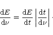 |
(1) |
It is worth mentioning that in spite of (dE/dt) in the above equation being
the pulsar gravitational wave emission rate, the time variation of the frequency
is
fixed by the magnetic dipole emission, responsible for the deceleration of
the star. This means that angular momentum losses by gravitational waves will
never
overcome those produced by magnetic torques, which is equivalent to say that
the average equatorial deformation is always less than 10-3.
Under these conditions, the energy frequency distribution, taking into account
that
the gravitational wave frequency is twice the rotational frequency is
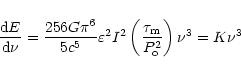 |
(2) |
where I is the moment of inertia of the star,
 is the magnetic braking
timescale (see RP00),
is the magnetic braking
timescale (see RP00),  is the initial period of the pulsar and the other
symbols have their usual meaning.
is the initial period of the pulsar and the other
symbols have their usual meaning.
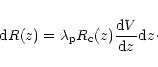
In order to estimate the average ratio
 ,
we adopted the
following
procedure. We have performed Monte Carlo simulations in which the distribution
probabilities of the variables
and
are the same as RP00.
The resulting distribution of the quantity log
is given in
Fig. 1, and it
can be fitted by a Gaussian with a mean equal to < log
,
we adopted the
following
procedure. We have performed Monte Carlo simulations in which the distribution
probabilities of the variables
and
are the same as RP00.
The resulting distribution of the quantity log
is given in
Fig. 1, and it
can be fitted by a Gaussian with a mean equal to < log
 =
12.544.
=
12.544.
Adopting this value as representative of the whole population,
the constant K in Eq. (2) is
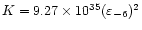 ergHz-4, where we have introduced the notation
 .
The gravitational wave flux at frequency
.
The gravitational wave flux at frequency
 (observer's frame) due to
sources localized in the redshift shell z,
(observer's frame) due to
sources localized in the redshift shell z,
 is
is
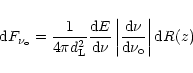 |
(3) |
where
 is the distance-luminosity, r is the proper distance and the
observer's frequency
is related to the frequency
is the distance-luminosity, r is the proper distance and the
observer's frequency
is related to the frequency  at the source by
 .
The event rate inside the shell z,
is
.
The event rate inside the shell z,
is
 |
(4) |
In the above equation,
 is the "cosmic'' star formation rate,
 is the mass fraction of formed
stars in the range 10-40
is the mass fraction of formed
stars in the range 10-40  ,
supposed to be the mass range
of the pulsar progenitors, with
,
supposed to be the mass range
of the pulsar progenitors, with  being the initial mass function.
For a Salpeter's law (
being the initial mass function.
For a Salpeter's law (
 ),
),
 .
The element of the comoving volume is
.
The element of the comoving volume is
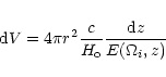 |
(5) |
where  is the Hubble parameter and the function
 is
defined by the equation
is
defined by the equation
 |
(6) |
where
 and
and
 are respectively the density parameters
due to matter (baryonic and non-baryonic) and the vacuum, corresponding
to a non-zero cosmological constant. The equivalent
density parameter due to the spatial curvature satisfies
are respectively the density parameters
due to matter (baryonic and non-baryonic) and the vacuum, corresponding
to a non-zero cosmological constant. The equivalent
density parameter due to the spatial curvature satisfies
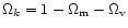 .
.
Combining these equations, the expected gravitational wave flux at the
frequency
is
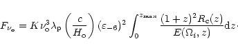 |
(7) |
In the literature an equivalent density parameter due to gravitational waves is
often used
to measure the strength of the background at a given frequency, defined by the
equation
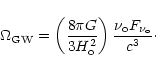 |
(8) |
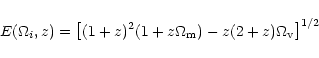
In order to evaluate numerically Eqs. (7)-(8), it is necessary to specify the
cosmic star formation rate
and the parameters of the world
model, namely, the values of ,
and
.
Madau & Pozzetti (1999) have reviewed the constraints imposed by the
observed extragalactic background light on the cosmic star formation rate
(CSFR). They
concluded that after an extinction correction of
A1500 = 1.2 mag
(
A2800 = 0.55 mag), a star formation rate given by the relation
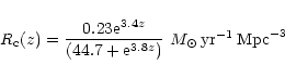 |
(9) |
fits all measurements of the UV-continuum and H luminosity densities
well
from the present epoch up to z = 4. However, according to Hopkins et al. (2001),
even when reddening corrections are taken into account, significant
discrepancies
still remain between the CSFR derived from UV-H
measurements and those
derived
from far-infrared and radio luminosities, which are not affected by dust
extinction.
Hopkins et al. (2001) assumed a reddening correction dependent on the star
formation
rate and obtained a good agreement between the CSFRs derived from different set
of
measurements. We have fitted their results by a function similar to Eq. (9),
namely,
luminosity densities
well
from the present epoch up to z = 4. However, according to Hopkins et al. (2001),
even when reddening corrections are taken into account, significant
discrepancies
still remain between the CSFR derived from UV-H
measurements and those
derived
from far-infrared and radio luminosities, which are not affected by dust
extinction.
Hopkins et al. (2001) assumed a reddening correction dependent on the star
formation
rate and obtained a good agreement between the CSFRs derived from different set
of
measurements. We have fitted their results by a function similar to Eq. (9),
namely,
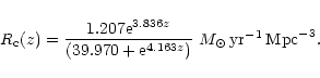 |
(10) |
Taking into account the uncertainties still present in the derivation of the
CSFR,
we have performed calculations using both rates.
Recent BOOMERANG and MAXIMA results (de Bernardis et al. 2000; Hanany et al.
2000) on
the power spectra of the cosmic microwave background and observations of distant
type
Ia supernovas (Perlmutter et al. 1999; Schmidt et al. 1998), which suggest that
the
expansion of the Universe is accelerating, support a spatially flat geometry and
a non-zero cosmological constant. Both sets of data are consistent with
 (including baryonic and non-baryonic matter) and
= 0.70, which will
be adopted
in our computations. However, no significant differences in our results were
observed if a model defined by
(including baryonic and non-baryonic matter) and
= 0.70, which will
be adopted
in our computations. However, no significant differences in our results were
observed if a model defined by
 and
and
 is adopted. The
Hubble parameter
was taken to be equal to 68 kms-1/Mpc-1
(Krauss 2001).
is adopted. The
Hubble parameter
was taken to be equal to 68 kms-1/Mpc-1
(Krauss 2001).
RP00 assume in their simulations that the maximum rotation frequency of a newly
born pulsar is 2000 Hz, which corresponds to a gravitational wave frequency of
4000 Hz. If the upper limit of the integral in Eq. (7) is
 ,
then
the maximum frequency seen by the observer is
,
then
the maximum frequency seen by the observer is  660 Hz. For higher
frequencies, only near objects will contribute to the integral and the upper
limit should be replaced by
660 Hz. For higher
frequencies, only near objects will contribute to the integral and the upper
limit should be replaced by
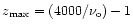 ,
with
in Hz. This
parameter affects the resulting spectrum, as we shall see below. Thus,
calculations
with a different cutoff were also performed.
,
with
in Hz. This
parameter affects the resulting spectrum, as we shall see below. Thus,
calculations
with a different cutoff were also performed.
Figure 2 shows the density parameter
 as a function of the
frequency.
Labels M1 and H1 correspond to star formation rates given respectively
by Eqs. (9) and (10) and a maximum gravitational wave frequency equal to
4000 Hz.
as a function of the
frequency.
Labels M1 and H1 correspond to star formation rates given respectively
by Eqs. (9) and (10) and a maximum gravitational wave frequency equal to
4000 Hz.
![\begin{figure}
\par\includegraphics[angle=-90,width=9cm,clip]{regimbau_1424.f2r.eps}
\end{figure}](/articles/aa/full/2001/35/aa1424/Timg49.gif) |
Figure 2:
Density parameter of GW versus frequency. Labels M and H
correspond respectively to cosmic star formation rates given by Eqs. (9) and (10), whereas labels 1 and 2 correspond to maximum rotation frequencies
of 2.0 and 1.0 kHz. The predicted background produced by distorted black holes
(Ferrari et al. 1999a) is also shown for comparison. |
| Open with DEXTER |
The labels M2 and H2 have the same meaning but here
the maximum gravitational wave frequency cutoff is at 2000 Hz,
corresponding to a minimum rotation period of 1ms. All these curves were
calculated for an equatorial deformation
 ,
and we
recall that the
results scale as
,
and we
recall that the
results scale as
 .
The numerical calculations indicate a broad
maximum around 1.5 kHz, if the maximum possible pulsar rotation frequency
is 2 kHz. Decreasing this limit by a half, the spectrum narrows and the maximum
shifts toward lower frequencies (
.
The numerical calculations indicate a broad
maximum around 1.5 kHz, if the maximum possible pulsar rotation frequency
is 2 kHz. Decreasing this limit by a half, the spectrum narrows and the maximum
shifts toward lower frequencies ( 0.9 kHz). The amplitude is also
affected, being
reduced by almost one order of magnitude. This happens because according
to Eq. (8), the amplitude grows as
0.9 kHz). The amplitude is also
affected, being
reduced by almost one order of magnitude. This happens because according
to Eq. (8), the amplitude grows as
 but a lower frequency cutoff
implies that only nearby objects will contribute to the integrated signal,
thus reducing the amplitude at maximum.
but a lower frequency cutoff
implies that only nearby objects will contribute to the integrated signal,
thus reducing the amplitude at maximum.
If the equatorial ellipticity may reach values of the order of 10-6,
then the energy density of the background generated by pulsars may be comparable
and even higher than that expected from newly born black holes (Ferrari et al.
1999a; de Araújo et al. 2000), originating from the collapse of massive stars
( 40 ). For a comparison, the spectrum corresponding to
the ring-down emission from distorted black holes calculated by Ferrari et al. (1999a) is also plotted in Fig. 2, appropriately scaled to the Hubble
parameter here adopted. In the case of distorted black holes, the
uncertainties on the estimates of the background energy density rest on
the conversion efficiency of the mass energy into gravitational waves as well as
on
the minimum mass of the progenitor.
40 ). For a comparison, the spectrum corresponding to
the ring-down emission from distorted black holes calculated by Ferrari et al. (1999a) is also plotted in Fig. 2, appropriately scaled to the Hubble
parameter here adopted. In the case of distorted black holes, the
uncertainties on the estimates of the background energy density rest on
the conversion efficiency of the mass energy into gravitational waves as well as
on
the minimum mass of the progenitor.
Hot and fast-rotating newly formed
neutron stars may be unstable against the r-mode instability. Ferrari
et al. (1999b) estimated that if all newly born neutron stars cross
the "instability window'' (see, for instance, Andersson et al. 2000), then
the resulting density parameter has a maximum amplitude of
 in the frequency range 0.5-1.7 kHz. This
signal would be by far the dominant component of the background at these
frequencies.
However, according to the simulations by RP00, only few pulsars are born
within the instability window, reducing the amplitude of
the background due to such a mechanism by orders of magnitude.
in the frequency range 0.5-1.7 kHz. This
signal would be by far the dominant component of the background at these
frequencies.
However, according to the simulations by RP00, only few pulsars are born
within the instability window, reducing the amplitude of
the background due to such a mechanism by orders of magnitude.
Unless the equatorial ellipticity of pulsars were substantially higher than
the present expectations, the background generated by rotating neutron
stars will hardly be detected by the present generation of laser
beam interferometers and/or resonant detectors, but this could be a possibility
for future projects presently under consideration, such as the Large
Scale Cryogenic Gravitational Wave Telescope (LCGT), sponsored by the University
of Tokyo and the European antenna EURO (W. Winkler, private communication). The
former,
with a baseline of 3 km, is expected to have
a 100 W laser and cooled sapphire mirrors among other technological improvements.
Therefore, one may expect that advanced laser beam interferometers may attain
in the near future a sensitivity around 1 kHz, corresponding to
a strain noise
 of about 10-25 Hz-1/2. On the other
hand,
the best strategy to detect the signal when the detector output is
dominated by the noise, which is the present case, is to correlate data from two
different gravitational antennas and to assume that they have independent noise.
One interesting possibility would be to correlate the output of such an advanced
detector with a resonant mass detector located at the same site, having a
spherical
or truncated icosahedron geometry. The advantages of this geometry
with respect to a longitudinal bar is that a free elastic sphere has five
degenerate quadrupole modes, each of which is sensitive to a different
polarization and wave direction. Moreover, for a given material and resonant
frequency, a spherical detector has a cross section larger than a cylindrical
one. The
sensitivity of resonant spheres is limited by Brownian motion noise associated
with dissipation in the antenna and transducer, as well as by the electronic
noise from amplifiers. In this case, the strain noise at resonance is
approximately
(Coccia & Fafone 1997)
of about 10-25 Hz-1/2. On the other
hand,
the best strategy to detect the signal when the detector output is
dominated by the noise, which is the present case, is to correlate data from two
different gravitational antennas and to assume that they have independent noise.
One interesting possibility would be to correlate the output of such an advanced
detector with a resonant mass detector located at the same site, having a
spherical
or truncated icosahedron geometry. The advantages of this geometry
with respect to a longitudinal bar is that a free elastic sphere has five
degenerate quadrupole modes, each of which is sensitive to a different
polarization and wave direction. Moreover, for a given material and resonant
frequency, a spherical detector has a cross section larger than a cylindrical
one. The
sensitivity of resonant spheres is limited by Brownian motion noise associated
with dissipation in the antenna and transducer, as well as by the electronic
noise from amplifiers. In this case, the strain noise at resonance is
approximately
(Coccia & Fafone 1997)
 |
(11) |
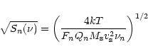
where k is the Boltzmann constant, T is the sphere temperature, Fn is
a dimensionless coefficient depending on each quadrupole mode (F1 =
2.98, F2 = 1.14, F3 = 0.107), Qn is the quality factor of the mode,
 is the mass of the sphere,
  is the
velocity of the sound and
is the
velocity of the sound and  is the mode frequency. For practical purposes,
let us consider a sphere constituted of the aluminium alloy Al-5056. This
material has a sound velocity of 5440 ms-1 and Coccia et al. (1996)
have reported Q values as high as 108 for temperatures below 100 mK. A sphere
with a diameter of 3.5 m (mass of 60.3 tons) has the two main frequencies
of the quadrupole modes at 0.8 kHz and 1.5 kHz,
covering quite well the predicted interval where the maximum amplitude of the
pulsar background should occur. Assuming a typical temperature of 20 mK, the
expected
strain noise derived from Eq. (11) is
is the mode frequency. For practical purposes,
let us consider a sphere constituted of the aluminium alloy Al-5056. This
material has a sound velocity of 5440 ms-1 and Coccia et al. (1996)
have reported Q values as high as 108 for temperatures below 100 mK. A sphere
with a diameter of 3.5 m (mass of 60.3 tons) has the two main frequencies
of the quadrupole modes at 0.8 kHz and 1.5 kHz,
covering quite well the predicted interval where the maximum amplitude of the
pulsar background should occur. Assuming a typical temperature of 20 mK, the
expected
strain noise derived from Eq. (11) is
 1.510-24 Hz-1/2.
If
 20 Hz is the bandwidth of the resonant mass detector and
 is the integration time, then the expected optimized signal-to-noise S/N
of
the correlated outputs is (Allen 1997)
is the integration time, then the expected optimized signal-to-noise S/N
of
the correlated outputs is (Allen 1997)
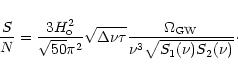 |
(12) |
For one year integration, one obtains from the equation above
 ,
indicating that new technology detectors may in the future reach the required
sensitivity to detect such a signal.
,
indicating that new technology detectors may in the future reach the required
sensitivity to detect such a signal.
The contribution of rotating neutron stars to the extragalactic background of
gravitational waves was calculated, under the assumption that the parameters
characterizing the galactic population of pulsars derived by RP00
are the same everywhere.
The amplitude of the equivalent density parameter attains a maximum in
the frequency interval 0.9-1.5 kHz and is in the range 10-11 to
310-9. The amplitude scales as
and, for a given
equatorial
ellipticity, the main uncertainties in the amplitude are essentially due to the
cosmic star formation rate and to the rotation frequency limit at the
pulsar birth, which depends on the equation of state of the nuclear matter. For
"realistic'' equations of state, these limits are in the rotation period range
0.5-1.0
ms, values adopted in our calculations.
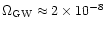
The present estimates indicate that this background, having a duty cycle
(measured by the product of the typical duration of the signal and the
mean birth frequency of pulsars) greater than one, may have an energy density
comparable to that produced by ''ring-down'' black holes. This emission is
unlikely to be
detected by the present generation of detectors. Correlated advanced detectors
may reach a limit of about
 10-10
for a flat spectrum (Maggiore 2000), which is not the present case.
However,
new technology detectors, which are presently under consideration, may
attain the required sensitivity. In particular, taking into account the
low cost of a resonant mass detector compared to that of a laser
interferometer,
the installation in the same site of a "sphere'' operating near the
maximum predict frequency (0.9-1.5 kHz), could be an adequate strategy
to detect such a signal in the future.
10-10
for a flat spectrum (Maggiore 2000), which is not the present case.
However,
new technology detectors, which are presently under consideration, may
attain the required sensitivity. In particular, taking into account the
low cost of a resonant mass detector compared to that of a laser
interferometer,
the installation in the same site of a "sphere'' operating near the
maximum predict frequency (0.9-1.5 kHz), could be an adequate strategy
to detect such a signal in the future.
-
Allen, B. 1997, in Relativistic Gravitation and Gravitational Radiation, ed.
J.-A. Marck, & J.-P. Lasota (Cambridge University Press), 373
In the text
-
Andersson, N, Jones, D. I., Kokkotas, K. D., & Stergioulas, N. 2000, ApJ, 534, 75
In the text
-
Blair, D. G., Burman, R., Woodings, L. J. S., Mulder, M., & Zadnik, M. G. 1997, in
Omnidirectional Gravitational Radiation Observatory, ed. W. F. Velloso,
O. D. Aguiar, & N. S. Magalhães (World Scientific), 251
In the text
-
Coccia, E., Fafone, V., Frossati, G., ter Haar, E., & Meisel, M. W. 1996, PRLA, 219, 263
In the text
-
Coccia, E., & Fafone, V. 1997, in Omnidirectional Gravitational Radiation Observatory,
ed. W. F. Velloso, O. D. Aguiar, & N. S. Magalhães (World Scientific), 113
In the text
-
de Araújo, J. C. N., Miranda, O. D., & Aguiar, O. D. 2000, PRD 61, 124015
In the text
-
de Bernardis, P., et al. 2000, Nature, 404, 995
In the text
-
de Freitas Pacheco, J. A., & Horvath, J. E. 1997, PRD, 56, 859
In the text
-
Ferrari, V., Matarrese, S., & Schneider, R. 1999a, MNRAS, 303, 247
In the text
NASA ADS
-
Ferrari, V., Matarrese, S., & Schneider, R. 1999b, MNRAS, 303, 258
NASA ADS
-
Giazotto, A., Bonazzola, S., & Gourgoulhon, E. 1997, PRD, 55, 2015
In the text
-
Hanany, S., et al. 2000, ApJL, 545, 5
In the text
-
Hopkins, A. M., Connoly, A. J., Haarsma, D. B., & Cram, L. E. 2001 [astro-ph/0103253]
In the text
-
Krauss, L. M. 2001 [astro-ph/0102305]
In the text
-
Madau, P., & Pozzetti, L. 1999, MNRAS, 312, 9
In the text
-
Maggiore, M. 2000, Phys. Rep., in press [gr-qc/9909001]
In the text
-
Owen, B. J., Lindblom, L., Cutler, C., et al. 1998, PRD, 58, 084020
In the text
-
Perlmutter, S., et al. 1999, ApJ, 517, 565
In the text
NASA ADS
-
Regimbau, R., & de Freitas Pacheco, J. A. 2000, A&A (RP00)
In the text
-
Schmidt, B., et al. 1998, ApJ, 507, 46
In the text
NASA ADS
-
Schutz, B. 1991, in The Detection of Gravitational Waves, ed. D. B. Blair
(Cambridge University Press)
In the text
Copyright ESO 2001
![\begin{figure}
\par\includegraphics[angle=-90,width=9cm,clip]{regimbau_1424.f1r.eps}
\end{figure}](/articles/aa/full/2001/35/aa1424/img13.gif)
![\begin{figure}
\par\includegraphics[angle=-90,width=9cm,clip]{regimbau_1424.f2r.eps}
\end{figure}](/articles/aa/full/2001/35/aa1424/img49.gif)