 Scuti stars in Praesepe
![[*]](/icons/foot_motif.gif)
A&A 376, 175-187 (2001)
DOI: 10.1051/0004-6361:20010950
Scuti stars in PraesepeS. Frandsen
1 -
A. Pigulski2 -
J. Nuspl3 -
M. Breger4 -
J. A. Belmonte5 -
T. H. Dall1 -
T. Arentoft6 -
C. Sterken6,
-
T. Medupe7 -
S. K. Gupta8 -
F. J. G. Pinheiro9 -
M. J. P. F. G. Monteiro9 -
C. Barban10 -
M. Chevreton11 -
E. Michel10 -
J. M. Benko3 -
Sz. Barcza3 -
R. Szabó3 -
Z. Ko aczkowski2 -
G. Kopacki2 -
S. N. Udovichenko12
1 - Institute for Physics and Astronomy, University of Aarhus,
Universitetsparken, Bygn. 520,8000 Aarhus C, Denmark
2 -
Institute of Astronomy, Wrocaw University, Kopernika 11,
51-622 Wrocaw, Poland
3 -
Konkoly Observatory, 1525 Budapest XII, PO Box 67, Hungary
4 -
Institut für Astronomie, Türkenschanzstrasse 17,
1180 Wien, Austria
5 -
Instituto de Astrofísica de Canarias, 38200 La Laguna,
Tenerife, Spain
6 -
Astronomy Group, University of Brussels (VUB), Pleinlaan 2,
1050 Brussels, Belgium
7 -
South African Astronomical Observatory, PO Box 9, Observatory
7935, Cape, South Africa
8 -
UP State Observatory, Manora Peak, Nainital - 263 129,
India
9 -
Centro de Astrofísica da Universidade do Porto, rua
das Estrelas, 4150-762 Porto, Portugal
10 -
Observatoire de Paris, DASGAL, UMR 8633, 92195 Meudon,
France
11 -
Observatoire de Paris, DAEC, UMR 8632, 92195 Meudon, France
12 -
Odessa Astronomical Observatory, Park Shevchenko, Odessa
270014, Ukraine
Received 20 April 2001 / Accepted 27 June 2001
Abstract
We present the results of the multisite differential CCD
photometry for the two Scuti stars, BN and BV Cnc, in the
open cluster Praesepe. The main objective was to identify the
character of the pulsation modes in BN Cnc deriving their accurate
periods, amplitudes and phases. These parameters are essential for
the mode identification which uses combined photometric and
spectroscopic data and is presented in the second article. For
BN Cnc, six pulsation modes with amplitudes above the detection limit
( 0.5 mmag) were detected. Using the same CCD frames it was
possible to verify the presence of the four pulsation modes in BV Cnc,
the faintest of
Scuti stars in Praesepe. It is shown that in
this very low-amplitude pulsator, substantial amplitude variations are
seen between 1997 and 1998.
0.5 mmag) were detected. Using the same CCD frames it was
possible to verify the presence of the four pulsation modes in BV Cnc,
the faintest of
Scuti stars in Praesepe. It is shown that in
this very low-amplitude pulsator, substantial amplitude variations are
seen between 1997 and 1998.
Key words: stars: oscillations - stars: variable:
Scuti - open clusters and associations: individual:
Praesepe
Current efforts to improve the understanding of stellar evolution
include asteroseismology as the most promising technique. Several
space programs are underway. COROT (Baglin et al. 2001) and
MONS (Kjeldsen et al. 2000) mainly address observations of
solar-like oscillations, whereas MOST (Matthews et al. 2001)
will observe also pulsators with higher amplitudes. All projects have
among their main targets one or more Scuti stars. The rich
set of oscillation modes in these stars make them very attractive for
seismic investigations.
Ground-based observations play a particularly important part in the
studies of this group of stars. Even though Scuti stars with
20-30 modes are observed, the comparison and identification of these
modes with model frequencies has proven to be very difficult. Two
methods have been attempted in order to solve this:
Scuti stars in
the open cluster Praesepe, where a series of photometric campaigns
have taken place (see below) and the Pleiades (Fox Machado et al. 2001). A quite clear dependence of the frequency
content on luminosity for Scuti stars in Praesepe (Belmonte
et al. 1997) indicates that the method can indeed be
successful.
If a good model can be found for one star (BN Cnc) and accurate parameters determined, then all common parameters (distance, [Fe/H], age) can be transferred to the 13 other variables, putting strong constraints on possible models for these stars.
Scuti stars in Praesepe - status
Praesepe has a nice group of Scuti stars consisting of 14 members (Rodríguez et al. 2000). For eight of these
stars (not including BV Cnc) models are discussed by Michel et al. (1999) and the frequencies and amplitudes are summarized
by Belmonte et al. (1997) and Hernández et al. (1998b, 1998c). Out of all
Scuti
stars in Praesepe, nine have been the targets of multisite
observations. BU and EP Cnc were observed by the DSN (Delta Scuti
star Network) (Breger et al. 1993, 1994). The
STEPHI team observed BU, BN Cnc and KW 284 (Belmonte et al. 1994)
and later BQ and BW Cnc (Álvarez et al. 1998) and BS and
BT Cnc (Hernández et al. 1998a). Finally, BN Cnc and BV Cnc
were observed by Arentoft et al. (1998), but
only from a single site. All the stars listed have been shown to be
multimode pulsators.
The STACC 1998 campaign on BN and BV Cnc is the first large-scale
photometric campaign based (mainly) on the differential CCD photometry
aimed at
Scuti stars. Using CCD cameras one can observe both
stars simultaneously.
Ten sites participated in the photometric observations, which took place from January to April 1998. A variety of instrumentation was used and the number of nights allocated varying from a few nights to several weeks.
The number of useful nights was considerably lower than expected due to an unusual bad observing season at several sites. In Fig. 1 the nights with data are shown schematically for the participating sites (photometry only). In addition, spectroscopic data were obtained at five observatories. The main part of observing took place in February 1998. The distribution of sites did not provide a good 24-hour coverage. In Table 1 the instrumentation and observations are described in detail.
![\begin{figure}
\par\includegraphics[width=8.4cm,clip]{h2827f1.ps}\end{figure}](/articles/aa/full/2001/34/aah2827/img5.gif) |
Figure 1: Distribution of the photometric observations of BN Cnc carried out during the 1998 STACC campaign. Five consecutive nights are shown in each row. |
| Open with DEXTER | |
| Telescope | Filter(s) | Field of | Nights | Hours | |||
| Observatory | diam. [cm] | Detector | used | view | observed | obtained | Remarks |
| Uttar Pradesh (India) | 100 | CCD | V | 6.6
 6.6 6.6 |
6 | 15.5 | guiding problems |
| Konkoly (Hungary) | 100 | CCD | V | 5.3
4.6 |
12 | 57.0 | |
| 60 | CCD | V | 27
18 |
5 | 17.8 | ||
| Biaków (Poland) |
60 | CCD | V | 6
4 |
8 | 32.0 | |
| Teide (Spain) | 80 | CCD | V | 7.3
7.3 |
9 | 59.0 | |
| Sutherland (S. Africa) | 100 | CCD |
 |
3.4
3.1 |
10 | 22.3 | |
| ESO, La Silla (Chile) | 90 | CCD | y | 3.9
3.9 |
12 | 11.5 | |
| Vienna APT (AZ, USA) | 75 | PM | v,y | -- | 7 | 46.4 | |
| La Palma (Spain) | 100 | CCD | V | 5.6
5.6 |
3 | 7.2 | |
| Haute Provence (France) | 80 | CCD | V | 6.4
6.4 |
2 | 5.2 | overexposed |
| Odessa (Ukraine) | 50 | CCD | V | 20
20 |
2 | 2.6 | high noise |
All sites except the Vienna APT in Arizona were using CCD cameras, but
with quite a range in field of view and filters. A Johnson V filter
was used at the majority of sites. At some sites (Sutherland, La
Silla, Arizona) the observations were carried out in other filters
(Strömgren vby, Cousins  ). The differences in fields
of view are best illustrated by displaying the two extreme cases.
Figure 2 shows a CCD frame obtained at Sutherland, while
Fig. 3 features a much larger field representing a frame
from the 60-cm Schmidt telescope at Piszkésteto in Hungary. The
latter clearly supplies a much larger set of reference stars for the
two variable stars. The two variables both have close fainter stars,
which in most cases are used as reference stars. These fainter stars
are uncomfortably close, as a certain defocusing was needed to permit
exposure times that give a decent duty cycle.
). The differences in fields
of view are best illustrated by displaying the two extreme cases.
Figure 2 shows a CCD frame obtained at Sutherland, while
Fig. 3 features a much larger field representing a frame
from the 60-cm Schmidt telescope at Piszkésteto in Hungary. The
latter clearly supplies a much larger set of reference stars for the
two variable stars. The two variables both have close fainter stars,
which in most cases are used as reference stars. These fainter stars
are uncomfortably close, as a certain defocusing was needed to permit
exposure times that give a decent duty cycle.
![\begin{figure}
\par\includegraphics[width=5.35cm,clip]{h2827f2.ps}\end{figure}](/articles/aa/full/2001/34/aah2827/img10.gif) |
Figure 2: A sample CCD frame of BN and BV Cnc field observed with the 1.0-m telescope at Sutherland Observatory. The two variables are labeled. North is up, east to the left. |
| Open with DEXTER | |
![\begin{figure}
\par\includegraphics[width=8.8cm,clip]{h2827f3.ps}\end{figure}](/articles/aa/full/2001/34/aah2827/img11.gif) |
Figure 3: A sample CCD frame observed with the 60-cm Schmidt telescope at Konkoly Observatory. |
| Open with DEXTER | |
Some additional details on the observations at different sites are given here in separate paragraphs.
The large field of view and the corresponding larger set of bright comparison stars obtained with the Schmidt telescope has the effect that better results are obtained with the 0.6-m than with the 1.0-m telescope (see later in Table 4). For the data coming from all other telescopes in the campaign equipped with CCD, stars fainter than the target stars BN and BV Cnc had to be used as comparisons.
ków Observatory.
Observations were carried out in three Strömgren filters v, b, yplus the Cousins
filter.
The best signal-to-noise (S/N) was obtained in the v and b bands, where a larger amplitude more than compensates for the smaller number of photons. This is so much more true, because systematic effects dominate the noise budget making it almost colour independent.
1k CCD was used. Time
was available a few hours on selected nights during another observing
program, and data were collected early in the campaign on 12 nights.
The longest set is only 2 hours long.
Weather conditions were variable and the quality varies quite a lot from night to night. Observing took place at large air masses and the telescope did not produce nice ringformed images when defocused, making the photometry difficult.
 C and has a typical dark current of 20 counts s-1. A
detailed description of the APTs and the attached equipment can be
found in the paper by Strassmeier et al. (1997).
C and has a typical dark current of 20 counts s-1. A
detailed description of the APTs and the attached equipment can be
found in the paper by Strassmeier et al. (1997).
The telescopes have been used before in the campaigns on other
Scuti stars with the three-star technique of alternating
observations of the variable star and two comparison stars. This
technique allows for a check of the accuracy of the measurements. For
the star 4 CVn, Breger & Hiesberger (1999) found a precision of
3.0 mmag in y for all three stars. For a 9th magnitude star,
BI CMi, the precision decreases to 3.8 mmag per single observation
under good weather conditions.
The whole month of February was allocated, but due to the poor weather the data were taken on only 7 nights and only for a substantial part of the night on 5 nights. This is much below normal.
As this is one of a few sites off European longitudes this is again disappointing and to some extent makes the multisite character of the campaign less useful.
The quality of the data varies dramatically with weather conditions and is overall somewhat more noisy than the CCD photometry.
![\begin{figure}
\par\includegraphics[width=2.2cm,clip]{h2827f4.ps}\end{figure}](/articles/aa/full/2001/34/aah2827/img13.gif) |
Figure 4: An example of an OHP image of the program stars. The stars are repositioned one above the other with the two target stars at the top and two reference stars at the bottom. |
| Open with DEXTER | |
Unfortunately, due to the trial nature of the observations, the variable stars were slightly overexposed and although some decorrelation was attempted, it did not bring the noise down to levels, where the data contribute significantly to the final result.
The windowing technique is interesting, because the duty cycle is higher than for other sites, and there is no reason to believe the results had been less good than from full frame observations had the overexposure not happened.
Only at a few sites was the number of clear nights a large fraction of the allocated time. This is often the case for northern observatories, especially in winter, except for the permanently good sites like the Canarian Islands or Hawaii. The Vienna APT site was considerably below normal owing to bad weather conditions caused by the El Niño.
It would clearly make this type of campaigns much more manageable, if telescopes and CCD cameras could be remotely operated in automatic or semi-automatic mode. In addition, telescopes should be situated at sites with a good photometric climate.
Most teams delivered completely reduced photometric time series for the two stars. Thus, several photometric reduction packages have been used. The choice has been made by the observing teams. In a couple of cases the raw data were transmitted and reduced by the PI.
The frames from Tenerife, ESO, OHP and UPSO were reduced using the differential photometry package MOMF (Kjeldsen & Frandsen 1992). The OHP frames were delivered as calibrated frames. The UPSO frames did not include an overscan strip. Bias frames had to be subtracted interpolating to the nearest in time. Due to the heavily defocused images, numerical binning had to be applied to some of the data to have the stellar diameters fitting the normal size of the Point Spread Function (PSF) in the MOMF package.
In addition to the magnitudes as a function of time, information about the image translation, the sky background and the seeing was recorded. Correlations with these household parameters or other parameters were checked and decorrelation attempted if dependencies were seen. This was absolutely needed for the OHP and UPSO data due to the problems described in the previous section.
The data from Vienna APT arrived as tables of magnitudes as a function of time for three stars: the two variable stars and a reference star. To reduce the effect of photon noise from the reference star on the differential magnitudes, a low-order smooth fit was made to the flux of the reference star, and this fit was then interpolated in time and subtracted from the two variable stars.
The Konkoly data were reduced by the method described by Arentoft et al. (1998) using a library of yet unpublished C functions.
The images from La Palma were reduced using DAOPHOT and the IRAF image
reduction tools. DAOPHOT was also used for the reduction of the
data from Biaków.
The CCD frames obtained at Sutherland were reduced using DoPhot, and finally no information is available on the reduction techniques employed at the Odessa site.
The reduced data represent differential magnitudes (with respect to one or more comparison stars, depending on the site) with a mean difference subtracted.
The light curves from the different sites and nights constitute a
rather inhomogeneous sample. Combining these data is far from
trivial. In order to see how some subjective decisions which must be
made at this stage affect the final result, the merging and
time-series analysis has been carried out independently by two teams
and the results compared.
It should be noted that the zero point corrections and detrending
we apply for our data at the merging state suppress all low-frequency
(2 d-1 and smaller) signals, both spurious and real, if such are
present.
Merging the data we try to correct for zero point offsets due to e.g. variable extinction and to adjust the scale in order to match different instrumental systems used at different sites.
The merging was done as an iterative process, where a number of free parameters were introduced and then fixed, either because a good value could be determined or a default value had to be chosen. Sometimes the datasets were too small or too noisy to allow for any but the simplest choice of parameters.
In the first step, the data made in b and v bands were transfered
to a common scale with V-filter using scaling ratios of
 and
and
 derived from Viskum et al. (1998) observations of FGVir. Because of the large
scatter, the -filter observations were not used. The yand V amplitudes were assumed to be identical. The data were next
divided into separate sets consisting of one-night observations from
each site.
derived from Viskum et al. (1998) observations of FGVir. Because of the large
scatter, the -filter observations were not used. The yand V amplitudes were assumed to be identical. The data were next
divided into separate sets consisting of one-night observations from
each site.
The parameters employed in the merging were then for each set: a correction for the zero point of the magnitude scale, a scaling factor (close to 1 and identical for all datasets with the same filter from one site) and a subjective quality factor, which was used to adjust weights applied in the time-series analysis.
Starting off with zero-point correction equal to zero, scaling factors of 1 and identical quality factors, a first fit of a light curve to the data was derived. Subtracting the current fit from the data points, zero points and scaling values were derived and used to replace the original parameters. Also, a weight for each data point was calculated based on a smoothed value of the rms deviation at each time. This weight was multiplied by the quality factor. Sigma clipping was also applied by giving zero weight to outliers.
The zero point offsets found were small and the scaling factors in most cases not significantly different from 1.0. The scaling from vand b to V with factors 1.24 and 1.44 was however slightly modified. A certain amount of subjective decisions entered into this process: when to stop iterations and freeze the parameter set.
Because the main effort has been to reduce the noise by improving the weights, several principles were used to derive weights:
 ,
and then decrease as the
deviation increases. We assumed that we have 2
equal to
8 mmag. Thus, all points with deviations less than 8 mmag get weights
1.0, but a 10 mmag deviation gets a weight of (8/10)2. The
threshold should not be chosen too low and one should not iterate too
many times as the solution then becomes unreliable.
,
and then decrease as the
deviation increases. We assumed that we have 2
equal to
8 mmag. Thus, all points with deviations less than 8 mmag get weights
1.0, but a 10 mmag deviation gets a weight of (8/10)2. The
threshold should not be chosen too low and one should not iterate too
many times as the solution then becomes unreliable.
aw, method 2
Because in method 1 scaling factors were found to be close to 1 for V and y observations, in the second approach no scaling of light curves made through different filters was performed. Since most of the data were obtained in Johnson V and Strömgren y bands, only these data were included. Because of different quality and sampling times, the emphasis was laid on a proper weighting of data. Low-quality nights were rejected from the analysis. Moreover, some data sets were freed from the instrumental low-frequency variations. This was done by fitting a sinusoid with a dominant frequency and allowing a linear time-dependent trend which was later subtracted.
![\begin{figure}
\par\includegraphics[width=8.7cm,clip]{h2827f5.ps}\end{figure}](/articles/aa/full/2001/34/aah2827/img18.gif) |
Figure 5: An example of the calculation of weights in method 2: Observatorio del Teide observations carried out on 1998 February 21/22. a) Observations (open circles), 0.008-day averages (filled circles), and smooth spline fit (continuous line). b) Residuals from the fit shown in panel a). For comparison, the weighting function (truncated Gaussian) is shown in scale. c) The weights (in arbitrary units). |
| Open with DEXTER | |
An example of the calculation of weights within method 2 is shown in
Fig. 5. The weights were assigned to each point
individually. As we wanted the weights to be inversely proportional
to the local variance, the procedure of calculating weigths was the
following. Firstly, the real light variations were fitted by
calculating averages in 0.008-day intervals and smoothing them by a
spline fit (Fig. 5a). The resulting residuals
(Fig. 5b) were next used to derive the local variance.
This variance was calculated in a common way, but additional weighting
of residuals was introduced in order to secure that only the points
closest to a given one contribute to the local variance. This
weighting function, a truncated Gaussian with
 d, is
also shown in Fig. 5b. Finally, weights were calculated,
as the inverse of the local variance multiplied by an arbitrary
scaling factor. As can be seen in Fig. 5c, the weights
indeed change accordingly with the changing scatter in residuals. We
also point out that this procedure includes no assumption on the
frequency content of the real signal.
d, is
also shown in Fig. 5b. Finally, weights were calculated,
as the inverse of the local variance multiplied by an arbitrary
scaling factor. As can be seen in Fig. 5c, the weights
indeed change accordingly with the changing scatter in residuals. We
also point out that this procedure includes no assumption on the
frequency content of the real signal.
As noted in the previous section, two independent time-series studies
of the BN and BV Cnc photometry have been carried out. The objective
is to find the best solution of the type
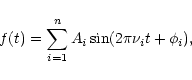 |
(1) |
 and the
phases
and the
phases  .
.
After cleaning the data with method 1, of the order of 7200 data points remained for BN Cnc and around 6800 for BV Cnc. To this we added about 620 points for BN Cnc and 680 for BV Cnc from 1997 obtained by Arentoft et al. (1998). The data from both seasons were combined together at the final stage of our analysis.
Periods, amplitudes and phases for a set of modes have been derived using the code Period98 (Sperl 1998) in its standard version and also in a version with a different weigthing scheme (see Sect. 5.1). In principle, Period98 uses Fourier periodogram and non-linear least-squares within its prewhitening process. In addition, the results from Period98 have been checked and special weighting procedures applied earlier by Frandsen et al. (1996) have been used.
![\begin{figure}
\par\includegraphics[width=12cm,clip]{h2827f6.ps}\end{figure}](/articles/aa/full/2001/34/aah2827/img23.gif) |
Figure 6: Selected nights of the 1998 photometry of BN and BV Cnc. The data were prepared according to method 1, the solid line corresponds to the fit taken from analysis 1 and given in Tables 2 and 3 for BN and BV Cnc, respectively. The number in each panel presents the HJD with 2450800 subtracted for the origin of the X-axis. Short tick marks are spaced 0.02 d. The tick marks on the Y-axis are separated by 5 mmag. The second label indicates the site(s) from which the data come: Bia - Biaków, open circles, Kon - Konkoly, plus signs, Sut - Sutherland, crosses, Ten - Tenerife, dots, and LaP - La Palma, squares. |
| Open with DEXTER | |
The data merged and weighted in a way described in Sect. 5.2 were used
in analysis 2. Because in this approach some observations from the
campaign were not used, the 1998 input dataset consisted of about 5000
data points for BN Cnc and rougly 4500 for BV Cnc. For 1997, the
numbers were approximately the same as in analysis 1. In analysis 2,
the least-squares (LS) periodogram allowing different weights was
applied. In principle, the
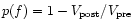 parameter plotted against the sample frequency f was used as a
periodogram. The
parameter plotted against the sample frequency f was used as a
periodogram. The
 and
and
 are the variances
calculated prior to (
)
and after (
)
fitting
a sinusoid with a given frequency f to the data. In addition, the
amplitude of a fitted sinusoid with frequency f was plotted as a
second periodogram (hereafter, this will be called the LS amplitude
periodogram). A detection of consecutive frequencies was done, like
in analysis 1, by prewhitening with all previously found frequencies.
are the variances
calculated prior to (
)
and after (
)
fitting
a sinusoid with a given frequency f to the data. In addition, the
amplitude of a fitted sinusoid with frequency f was plotted as a
second periodogram (hereafter, this will be called the LS amplitude
periodogram). A detection of consecutive frequencies was done, like
in analysis 1, by prewhitening with all previously found frequencies.
The consecutive steps of the prewhitening with both kinds of time-series analysis are shown in Figs. 7 and 8 for BN Cnc and BV Cnc 1998 data, respectively.
![\begin{figure}
\par\includegraphics[width=18cm,clip]{h2827f7.ps}\end{figure}](/articles/aa/full/2001/34/aah2827/img27.gif) |
Figure 7: Frequencies detected in the 1998 photometry of BN Cnc. The triangles indicate which frequencies were subtracted in the consecutive steps. Left: prewhitening process within analysis 1. These are Fourier periodograms. The spectral window is shown at the top panel. Right: the consecutive steps of prewhitening within analysis 2. The periodograms are the LS amplitude periodograms. The high peak at frequency 1 d-1 is an artifact produced by the method. |
| Open with DEXTER | |
![\begin{figure}
\par\includegraphics[width=18cm,clip]{h2827f8.ps}\end{figure}](/articles/aa/full/2001/34/aah2827/img28.gif) |
Figure 8: The same as in Fig. 7, but for the 1998 BV Cnc data. |
| Open with DEXTER | |
The final results seem to be fairly robust in terms of a good agreement between the sets of oscillating modes for each variable derived using different weights and different programs. Although there are 1 d-1 differences in case of BV Cnc, the frequencies are derived in the same sequence by both methods. There are, however, small differences which need to be commented.
For BN Cnc (Fig. 7) the two methods yield, within the
errors, the same frequencies F1 to F5. Although in analysis 2 the
alias peak at F1-1 d-1 is higher than F1, the analysis of the
combined 1997 and 1998 data (as well as the results from the STEPHI
campaign, which had a better spectral window, Belmonte et al. 1994) leaves no doubt that the true frequency is F1
 25.76 d-1, found as highest by analysis 1.
Consequently, a sinusoid with frequency F1 was subtracted in the first
step of prewhitening in analysis 2 as well. The largest difference
(
25.76 d-1, found as highest by analysis 1.
Consequently, a sinusoid with frequency F1 was subtracted in the first
step of prewhitening in analysis 2 as well. The largest difference
(
 0.044 d-1) was obtained for the last frequency
we derive, that is, F6. Again, combined 1997 and 1998 data indicate
that F6 = 25.4351 d-1 is the correct one. We note that these
different F6 frequencies are 1/
23-day aliases, and
23 d is the average time difference between our 1998 January/February,
late February and March groups of data (see Fig. 1). The amplitudes
found in analysis 1 and 2 agree within the 3
error, although,
on average, analysis 2 gives them higher by 0.13 mmag.
0.044 d-1) was obtained for the last frequency
we derive, that is, F6. Again, combined 1997 and 1998 data indicate
that F6 = 25.4351 d-1 is the correct one. We note that these
different F6 frequencies are 1/
23-day aliases, and
23 d is the average time difference between our 1998 January/February,
late February and March groups of data (see Fig. 1). The amplitudes
found in analysis 1 and 2 agree within the 3
error, although,
on average, analysis 2 gives them higher by 0.13 mmag.
For BV Cnc (Fig. 8) the situation is more confusing. As can be seen in Fig. 8, there is a strong aliasing problem for all three frequencies we find in the 1998 data. Like for BN Cnc, analysis 2 gives slightly higher amplitudes.
Because the results of analysis 1 and 2 are quite consistent (within the errors), we decided to present in a tabular form only the results of analysis 1. The differences we indicated above give an evaluation of the systematic errors which can be introduced at the subjective stage of merging and weighting the data of different quality.
To illustrate the data, selected nights are displayed in Fig. 6 together with the best fit found. On some dates data come from two sites.
The result of our analysis is an unambiguous determination of a small set of frequencies in BN and BV Cnc, and a low upper limit on the amplitudes of possible additional modes. We now comment in detail the frequency spectra of both stars and compare them with previous studies.
For this star we detect six modes. Five of them were known before and only one additional mode (F6) is new in comparison to earlier measurements (Belmonte et al. 1994; Arentoft et al. 1998). With the new dataset any alias problems have disappeared. Even though the sidelobes are still there, the S/N (see Table 2) is so good that there is no room for ambiguity. The frequency resolution is so high that it is improbable that any unresolved modes will be found.
| Our | Former | Frequency | Amplitudes [mmag] | Phase |  (97) (97) |
|||||
| ID | ID | [d-1] | [ Hz] Hz] |
1992 | 1997 | 1998 | 1997+1998 | [rad] | S/N | [Hz] |
| F1 | A4 | 25.76114(04) | 298.1614(05) | 2.0 | 2.00(27) | 3.01(8) | 2.92(7) | 4.87(03) | 26 | 298.01 |
| F2 | A2 | 23.02981(05) | 266.5487(05) | 2.1 | 2.08(26) | 2.52(8) | 2.48(7) | 1.70(03) | 20 | 266.42 |
| F3 | A8 | 28.27039(05) | 327.2036(05) | 2.7 | 1.99(23) | 2.42(8) | 2.38(7) | 3.08(03) | 23 | 327.16 |
| F4 | A1 | 22.78352(05) | 263.6981(06) | 1.2 | 1.80(27) | 2.32(8) | 2.29(7) | 5.08(03) | 17 | 263.69 |
| F5 | A5 | 25.93964(05) | 300.2273(06) | 0.9 | 2.33(25) | 2.13(8) | 2.13(7) | 3.87(03) | 24 | 300.24 |
| F6 | - | 25.43666(17) | 294.4057(19) | -- | 0.92(24) | 0.63(8) | 0.67(7) | 1.88(11) | 6 | -- |
Table 2 lists the modes we have detected with references to the analysis of Arentoft et al. (1998) indicated. Within the uncertainities, the amplitudes of the five dominant modes (except maybe F1) seem to be constant from 1997 to 1998. Two modes (F4 and F5) were weaker during the STEPHI campaign in 1992 and have increased amplitudes by roughly a factor of two. STEPHI had one more significant mode (A3) which, however, is different from the F6 mode. Two additional frequencies (A6 and A7) are listed by Arentoft et al. (1998), both with S/N < 3.0 in 1997 data, and none of them was recovered in the present larger dataset.
The noise level we obtained is around 0.12 mmag on the short side of the oscillation frequencies in the interval 8-15 d-1 and decreases to a white noise level of 0.07 mmag around 45 d-1. Modes with amplitudes above 0.5 mmag should be therefore detectable. For the rereduction of the STEPHI data, the corresponding noise levels were 0.17 mmag and 0.11 mmag (Arentoft et al. 1998). After removal of six modes, the residuals show only a small excess just below 30 d-1, indicating either some non-detected modes or perhaps inadequate removal of the signal. If there were indeed more modes with amplitudes just below the detection limit, including these modes into the solution would probably change the results for the largest-amplitude modes in an unsignificant way.
By varying weights and by adding a few more modes, we have found rough
estimates of the systematic errors on the detected modes. From
Table 4 it follows, using the relation
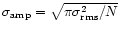 ,
that not counting points with low
weights and taking N = 6000 and
,
that not counting points with low
weights and taking N = 6000 and
 = 0.003 mmag, we
get a noise in the amplitude spectrum of
= 0.003 mmag, we
get a noise in the amplitude spectrum of
 0.07 mmag. With the typical amplitude of the modes in
BN Cnc of 2.5 mmag, we expect a
0.07 mmag. With the typical amplitude of the modes in
BN Cnc of 2.5 mmag, we expect a
 or an error in the
amplitudes of 3%. The S/N in Table 2 are derived from an
averaged noise in the residual amplitude spectrum. The values in
Table 2 are lower than 35, because of the excess power in
the range of the pulsation modes compared to the high frequency part
of the spectrum.
or an error in the
amplitudes of 3%. The S/N in Table 2 are derived from an
averaged noise in the residual amplitude spectrum. The values in
Table 2 are lower than 35, because of the excess power in
the range of the pulsation modes compared to the high frequency part
of the spectrum.
Montgomery and O'Donoghue (1999) have derived analytical
error formulas for least squares fits. With the same parameters as above
and T = 10 months we find using their Eqs. (4), (10) and (11):
 mmag,
mmag,
 Hz and
 rad. The errors of the amplitude,
frequency and phase given in Table 2 are only slightly higher
than those obtained from the analytical predictions.
rad. The errors of the amplitude,
frequency and phase given in Table 2 are only slightly higher
than those obtained from the analytical predictions.
This star was shown to be a multimode Scuti star by Arentoft
et al. (1998), where four modes are listed. We have
reanalyzed the 1997 data and found somewhat lower amplitudes (see
Table 3). One night was rejected and the remaining nights
were detrended to remove obvious drift problems. New weights were
calculated and bad points rejected. Arentoft et al. (1998)
also cleaned the data before deriving their amplitudes.
In 1998 data we find three frequencies (Fig. 8). Owing to the low amplitudes and the shape of our spectral window, an 1 d-1ambiguity in the derived frequencies remains. The frequencies F1 to F3 reported in Table 3 were derived from the combined 1997 and 1998 dataset and then refined by the non-linear least-squares. At the residual periodograms of 1998 data (bottom ones in Fig. 8), F4 can be barely visible. It is, however, obvious that this frequency was present in 1997 data, which can be judged from the bottom panel of Fig. 9 showing the periodogram for 1997 data after removing the first three frequencies. Therefore, we included F4 = 20.246 d-1, which is an 1 d-1alias of A3 derived by Arentoft et al. (1998), as the fourth frequency for BV Cnc.
At the same time, we can clearly see (Fig. 9, Table 3) that not only F4, but amplitudes of all four modes have
decreased between 1997 and 1998. In addition, more low-amplitude ( 0.5 mmag) modes can be present in the 1998 data because of the
excess of power at the residual periodograms (Fig. 8) in
the range between 15 and 28 d-1. Their amplitudes are close to
the detection limit, so we can only indicate the most promising
candidate. This is the peak at frequency of 17.77 d-1.
0.5 mmag) modes can be present in the 1998 data because of the
excess of power at the residual periodograms (Fig. 8) in
the range between 15 and 28 d-1. Their amplitudes are close to
the detection limit, so we can only indicate the most promising
candidate. This is the peak at frequency of 17.77 d-1.
| Our | Former | Frequency | Amplitudes [mmag] | Phase | (97) |
|||
| ID | ID | [d-1] | [Hz] |
1997 | 1998 | [rad] | S/N | [Hz] |
| F1 | A1 | 16.45039(06) | 190.3980(07) | 2.21(26) | 1.45(9) | 0.33(06) | 7.1 | 190.47 |
| F2 | A2 alias | 16.73053(08) | 193.6404(09) | 1.47(25) | 1.08(9) | 2.60(08) | 5.3 | 204.83 |
| F3 | A4 alias | 32.90896(10) | 380.8907(12) | 1.15(23) | 0.79(8) | 5.30(11) | 4.9 | 369.10 |
| F4 | A3 alias | 20.246(4) | 234.33(5) | 2.18(23) | 0.52(8) | 4.77(16) | 3.7 | 222.65 |
![\begin{figure}
\par\includegraphics[width=8.75cm,clip]{h2827f9.ps}\end{figure}](/articles/aa/full/2001/34/aah2827/img40.gif) |
Figure 9: The evidence for the amplitude change in BV Cnc. Top: LS amplitude spectrum for 1998 data from analysis 2. Middle: the same for 1997 data. Bottom: LS amplitude periodogram of the 1997 data after removing the F1 to F3 frequencies. Note that F4 = 20.246 d-1 clearly stands above the noise level. |
| Open with DEXTER | |
The results fall in two categories: the technical or observational aspects and the scientific progress made in this project.
Table 4 presents two values for the rms deviation of each datapoint from the final solution for the lightcurve of BN Cnc for each site, as well as the total weight of the dataset as applied in the analysis of the combined time series. The first rms entry is calculated giving equal weight to each point, whereas the second applies the weight used for analysing the lightcurve. Poor measurements enter fully into the first, but are eliminated in the second value. The difference reflects the extent to which the data has been cleaned and weighted.
| Observatory | RSD1 | RSD2 | Contr. |
| [mmag] | [mmag] | % | |
| Tenerife | 2.91 | 2.13 | 32.0% |
| Arizona APT | 5.61 | 3.35 | 17.5% |
| Konkoly (60 cm) | 2.89 | 2.42 | 12.3% |
| Konkoly (100 cm) | 4.95 | 3.49 | 8.5% |
| Biaków |
3.85 | 3.44 | 8.2% |
| Sutherland | 5.44 | 3.03 | 5.5% |
| ESO | 4.87 | 3.97 | 4.0% |
| La Palma | 4.95 | 3.45 | 1.5% |
| UPSO | 8.79 | -- | 0.4% |
| Odessa | 12.08 | -- | 0.2% |
| OHP | -- | -- | 0.0% |
| 1998 data | 4.55 | 2.88 | 90.1% |
| 1997 data | 3.94 | 3.11 | 9.9% |
Looking at Table 4 it is evident that a few sites dominate, partly because of the number of contributed nights, but also due to a higher accuracy for each datapoint.
A few participating sites did not reach the expected accuracy. The distributed observational guidelines obviously were not well enough prepared, that all sites understood the procedures that need to be followed in order to get high quality data. In some cases the instrumentation was not adequate (no autoguider, no overscan of the CCD etc.).
It is also evident that the best CCD photometry outperforms the APT
with a photoelectric photometer, which is how it ought to be given
that the quantum efficiency of CCDs are higher than for
photomultipliers. The factor is, however, small enough that the
Arizona site at a different longitude than the CCD sites is very
important, not to mention its ease of use. It must be also kept in
mind that weather conditions in Arizona were below normal. The value
from the third column of Table 4 corresponds well with the
values quoted in Sect. 3 obtained for other Scuti stars
observed with the APT in Arizona.
The sites providing multicolour data show a better S/N in the blue bands. It seems to be an advantage to observe in the B (or b) band instead of the V (or y) band. The increase in oscillation amplitude going from V to B makes up for the loss of the number of photons.
The window function we obtained (Fig. 7) does not really look like a multisite window function. The alias problem is anyway solved for BN Cnc star due to the presence of data distributed over several months and the low noise level achieved. The high frequency resolution obtained almost guarantees that all detected modes are single.
The noise level in the resulting spectra has been lowered in
comparison with earlier observations. It is comparable to the best
measurements of other Scuti stars. The mode content of the
two stars is consequently better defined than before. The presence of
some of the modes seen by Arentoft et al. (1998) in the
BN Cnc data has not been confirmed. This is important because the
parameters derived for BN Cnc depended on these presently undetected
modes. This is described in more detail in Paper II.
The amplitudes, frequencies and phases of the six BN Cnc modes are very well determined and provide an excellent baseline for the subsequent analysis of the spectroscopic timeseries presented in Paper II. There is a small bump in the residual noise spectrum in the range 26-30 d-1 for this star, but it is difficult to detect any unambiguous modes explaining the presence of this bump.
Evidently the amplitudes of BV Cnc modes have decreased from 1997 to 1998 which is probably best documented by Fig. 9. The difference diminished slightly when a reanalysis was done of the original 1997 data, but the change still remains at a non-ambiguous level. In BV Cnc the presence of several modes close to the detection limit is indicated by a very non-flat residual noise spectrum (see Fig. 8). Opposite to the case of BN Cnc, and due to the low amplitudes we measure, alias problems are quite severe.
It is interesting to note that for BV Cnc the difference between F3
and doubled F1 frequency is very small and amounts to 0.00822  .00016 d-1. This is almost exactly equal to 3 yr-1 =
0.00821 d-1. Since it could happen that both F1 and F3 are in
error by 1 or 2 yr-1, the possibility that F3 is a harmonic of F1
cannot be rejected. In that case the star would be quite unusual
because harmonics are rarely observed for such low-amplitude
pulsations. In case it is a pure coincidence, the two modes are very
close to the 2:1 resonance which may play an important role in their
behaviour.
.00016 d-1. This is almost exactly equal to 3 yr-1 =
0.00821 d-1. Since it could happen that both F1 and F3 are in
error by 1 or 2 yr-1, the possibility that F3 is a harmonic of F1
cannot be rejected. In that case the star would be quite unusual
because harmonics are rarely observed for such low-amplitude
pulsations. In case it is a pure coincidence, the two modes are very
close to the 2:1 resonance which may play an important role in their
behaviour.
It should be also pointed out that the two faintest Scuti
stars in Praesepe, BS Cnc observed by STEPHI (Hernández et al. 1998a) and BV Cnc, display a very similar pattern of
excited modes. Both have two or three modes in the range
between 15 and 20 d-1 and a single mode with frequency over
30 d-1. In other words, BV Cnc matches the pattern of the
luminosity dependence of the frequencies excited in Praesepe
Scuti stars, shown by Belmonte et al. (1997). This
means that studying Scuti stars in open clusters, especially
in Praesepe, could indeed help us to understand the nature of mode
selection, constrain cluster parameters and support the mode
identification. For this purpose, the work on the other, less
extensively observed Scuti stars in Praesepe, need to be
continued.
Scuti stars with noise levels of the order of 0.10-0.15 mmag allowing
detection of the modes with amplitudes larger than 0.5 mmag.
This is similar to the best campaigns for other
Scuti stars;
Acknowledgements
Part of this work was supported by the German Deutsche Forschungsgemeinschaft, DFG project number Ts 17/2-1. This work was also supported in part by grant in Portugal PESO/P/PRO/1196/97'' as well as by the Fund for Scientific Research (FWO) and by the Flemish Ministry for Foreign Policy, European Affairs, Science and Technology. M. Breger and the APT were supported by the Austrian Fonds zur Förderung der wissenschaftlichen Forschung. The IAC80 telescope is operated by the Instituto de Astrofísica de Canarias in the Spanish Observatorio del Teide. The Konkoly team thanks A. Frontó for his collaboration in the observations. The Porto team thanks A. Pedrosa for his collaboration with the observations.