3 Results

   
3.1 Data sample and light curves

The complete data sample consists of observations taken between December, 1996, and June, 2000. During these periods, the source was systematically observed in a range of zenith angle extending from close to the Zenith up to  $45\hbox{$^\circ$ }$. The intensity of the source did not influence the observation strategy. However, a selection based on criteria requiring clear moonless nights and stable detector operation has been applied: this leaves a total of 139 hours of on-source (ON) data, together with 57 hours on control (OFF) regions. The different light curves of the four observation periods are shown in Fig. 3. We used a differential index of -2.9, which is representative of all spectral measurements presented in Sect. 3.2, to estimate the integral flux above $250\:{\rm GeV}$ for all data, especially those taken far from the Zenith: this procedure is detailed in Appendix A.2.

As can be seen in Fig. 3, the flux of Mkn 421 changed significantly between 1996-97 and 1997-98: almost quiet during the first period (with a mean flux $\Phi_{>250\:{\rm GeV}}=2.5\pm0.9\times10^{-11}\:{\rm cm}^{-2}\:{\rm s}^{-1}$), the source showed a higher mean activity during the second period ( $\Phi_{>250\:{\rm GeV}}=6.0\pm0.6\times10^{-11}\:{\rm cm}^{-2}\:{\rm s}^{-1}$), with small bursts in January and March sometimes showing up in excess of the steady flux from the Crab nebula (which is $\Phi^{\rm CN}\equiv14.10\pm0.35\times10^{-11}~{\rm cm}^{-2}~{\rm s}^{-1}$ above $250~{\rm GeV}$, see Piron 2000). In 1998-99, the mean VHE emission of Mkn 421 ( $\Phi_{>250\:{\rm GeV}}=2.7\pm0.9\times10^{-11}~{\rm cm}^{-2}~{\rm s}^{-1}$) decreased to a level comparable to that of 1996-97. In spite of some activity detected during the winter, the weather conditions in Thémis caused a very sparse source coverage. Nevertheless in the beginning of 2000 Mkn 421 showed a remarkable increase in activity, exhibiting a series of huge bursts. As seen in Fig. 3, the bursts recorded in January and February 2000 clearly appear as the highest ever seen by CAT from this source in four years with a nightly-averaged integral flux culminating at $\sim$ $2\:\Phi^{\rm CN}$ and a large night-to-night variability.

VHE intra-night variability was also observed on a few occasions. For instance during the night of January 12-13, the source intensity increased by a factor of 3.8 in $\sim$2 hours, from $\sim$ $0.6\:\Phi^{\rm CN}$ to $\sim$ $2.3\:\Phi^{\rm CN}$(with a $\chi ^2$ per d.o.f of 2.5 for the absence of any variation), as can be seen in Fig. 3.1 (upper-left panel). At the bottom of this figure, Mkn 421 light curves are also shown for three nights from the 3rd to the 5th February. While the fluxes recorded by CAT during the first and last nights were stable, respectively $\Phi_{>250\:{\rm GeV}}\simeq1.3\:\Phi^{\rm CN}$ (over 4 hours) and $\Phi_{>250\:{\rm GeV}}\simeq0.7\:\Phi^{\rm CN}$ (over 1 hour), the source activity changed dramatically in a few hours during the second night (February 4-5). The CAT telescope started observation while the source emission was at a level of $5.5\:\Phi^{\rm CN}$. This flux is comparable to the historically highest ${\rm TeV}$ flux ever recorded, i.e., that of Mkn 501 during the night of April 16th, 1997 (Djannati-Ataï et al. 1999). In spite of the low source elevation ( $\theta_{\rm z}=44\hbox{$^\circ$ }$) 124 $\gamma$-ray events with a signal significance of $6.5\:\sigma$ were detected during the first 30 minutes of observation. This may be compared to the 838 $\gamma$-ray events and significance of $13.8\:\sigma$obtained during the whole night (see Fig. 1). After this first episode, the source intensity was reduced by a factor of 2 in 1 hour and by a factor of 5.5 in 3 hours. In Fig. 3.1, each point stands for a $\sim$ $30\:{\rm min}$ observation but a finer binning in time does not show any additional interesting features, confirming that CAT started observation after the flare maximum.

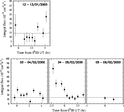Figure 4: Mkn 421 integral flux above $250\:{\rm GeV}$ during the night of January 12-13, 2000 (MJD 51555/56, left panel), and between 3 and 6 February, 2000 (MJD 51577 to 51580, lower panels). Each point stands for a $\sim$ $30\:{\rm min}$ observation and the dashed lines show the Crab nebula level emission $\:\Phi^{\rm CN}$.

   
3.2 1998 and 2000 time-averaged spectra

The data used in this section consist of a series of $\sim$ $30\:{\rm min}$ acquisitions for which a $\gamma$-ray signal with significance greater than $3\sigma$ was recorded, and they have been further limited to zenith angles $\theta_{\rm z}<28\hbox{$^\circ$ }$, i.e., to a configuration for which the detector calibration has been fully completed. The spectral study is thus based on 6.2 hours of on-source (ON) data taken in 1998 and 8.4 hours in 2000. Though this data selection reduces somewhat the total number of $\gamma$-ray events, it provides a high signal-to-noise ratio, minimizes systematic effects, and allows a robust spectral determination. Concerning systematic effects, another favourable factor is the low night-sky background in the field of view due to the lack of bright stars around the source.

Systematic errors are thus mainly due to the uncertainty on the absolute energy scale, which comes from possible variations of the atmosphere transparency and light-collection efficiencies during the observation periods. To a lesser extent, they are also due to limited Monte-Carlo statistics in the determination of the effective detection area. These errors, assumed to be the same for all spectra, are implicitly considered in the following and they have been estimated from detailed simulations (Piron 2000): $(\Delta\phi_0/\phi_0)^{\rm syst}=\pm20$%, $(\Delta\gamma)^{\rm syst}=\pm0.06$, and $(\Delta\beta)^{\rm syst}=\pm0.03$.

The 1998 and 2000 time-averaged spectra are shown in Fig. 5, both in the power-law and curved shape hypotheses. The statistics used for their extraction are detailed in Appendix B.1, the spectral parameters are summarized in Table 1, and their covariance matrices are given in Appendix B.2. In each panel of Fig. 5, the two lower plots give the ratio, in each bin of estimated energy, of the predicted number of events to that which is observed both for the $\gamma$-ray signal ($R_\gamma$) as well as for the hadronic background ($R_{\rm h}$). This is another means to check the validity of the parameters estimation, and to compare between the two hypotheses on the spectral shape.

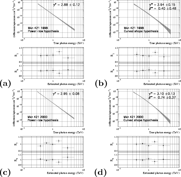Figure 5: Mkn 421 time-averaged spectra between 0.3 and $5.0\:{\rm TeV}$ in 1998 and 2000, for the power-law and curved shape hypotheses. The areas show the 68% confidence level contour given by the likelihood method. In each of the four panels, the two lower plots give the ratio, in each bin of estimated energy, of the predicted number of events to that which is observed both for the $\gamma$-ray signal ($R_\gamma$) as well as for the hadronic background ($R_{\rm h}$).

 

 

Table 1: Characteristics of the Mkn 421 spectra obtained in this paper. For each spectrum we indicate the observation period, the total energy band used in the likelihood method, $\Delta\widetilde{E_\gamma}$, the total observed number of $\gamma$-ray events, $S_\gamma$, the spectral parameters obtained in the $\mathcal{H}^{\rm pl}$ and $\mathcal{H}^{\rm cs}$ hypotheses, and the likelihood ratio $\lambda$. We also quote the decorrelation energy in the $\mathcal{H}^{\rm pl}$ hypothesis, $E_{\rm d}$, the energy $E^{\rm cs}_0$ at which the energy-dependent exponent $\gamma^{\rm cs}_l(E_{{\rm TeV}})=\gamma^{\rm cs}+\beta^{\rm cs}\log_{10}E_{{\rm TeV}}$has a minimal error in the $\mathcal{H}^{\rm cs}$ hypothesis (see Appendix B.2), and the corresponding value $\gamma ^{\rm cs}_0\equiv \gamma ^{\rm cs}_l(E^{\rm cs}_0)$. The energies are given in ${\rm TeV}$, and the flux constants in units of 10$^{-11}\:$cm^-2s^-1TeV^-1.

Period	${\Delta\widetilde{E_\gamma}\;({\rm TeV})}$	${S_\gamma}$	${\phi_0^{\rm pl}}$	${\gamma^{\rm pl}}$	${E_{\rm d}}$	${\phi_0^{\rm cs}}$	${\gamma^{\rm cs}}$	${\beta^{\rm cs}}$	${E^{\rm cs}_0}$	${\gamma^{\rm cs}_0}$	${\lambda}$
${1998}$	${0.3}-\scriptstyle{5.0}$	${735}\,\pm\,\scriptstyle{57}$	${2.29}\,\pm\,\scriptstyle{0.20}$	${2.88}\,\pm\,\scriptstyle{0.12}$	${0.69}$	${2.51}\,\pm\, \scriptstyle{0.32}$	${2.94}\,\pm\,\scriptstyle{0.15}$	${0.40}\,\pm\,\scriptstyle{0.48}$	${0.73}$	${2.88}\,\pm\,\scriptstyle{0.14}$	${0.75}$
${2000}$	${0.3}-\scriptstyle{5.0}$	${1424}\,\pm\,\scriptstyle{71}$	${2.90}\,\pm\,\scriptstyle{0.18}$	${2.95}\,\pm\,\scriptstyle{0.08}$	${0.63}$	${3.34}\,\pm\, \scriptstyle{0.28}$	${3.10}\,\pm\,\scriptstyle{0.13}$	${0.74}\,\pm\,\scriptstyle{0.37}$	${0.61}$	${2.94}\,\pm\,\scriptstyle{0.10}$	${4.90}$
${4-5/02/2000}$	${0.3}-\scriptstyle{2.0}$	${609}\,\pm\,\scriptstyle{40}$	${3.16}\,\pm\,\scriptstyle{0.34}$	${2.82}\,\pm\,\scriptstyle{0.15}$	${0.57}$	${3.25}\,\pm\, \scriptstyle{0.37}$	${3.08}\,\pm\,\scriptstyle{0.39}$	${0.63}\,\pm\,\scriptstyle{0.81}$	${0.37}$	${2.81}\,\pm\,\scriptstyle{0.17}$	${0.61}$

As can be seen in Fig. 5a, the power law accounts very well for the 1998 time-averaged spectrum. The likelihood ratio value is low ( $\lambda=0.75$, corresponding to a chance probability of 0.39), and the curvature term is compatible with zero ( $\beta^{\rm cs}=0.40\pm0.48^{\rm stat}$). Thus, we find the following differential spectrum:

$$\begin{eqnarray*}\frac{{\rm d}\phi}{{\rm d}E}&=&(2.29\pm0.20^{\rm stat}\pm0.46^{... ...times E_{{\rm TeV}}^{-2.88\pm0.12^{\rm stat}\pm0.06^{\rm syst}}. \end{eqnarray*}$$

On the contrary, Fig. 5d shows some evidence for a curvature in the 2000 time-averaged spectrum, with a relatively high likelihood ratio value ( $\lambda=4.90$, corresponding to a chance probability of 0.027). The lower plots of Fig. 5d, when compared to those of Fig. 5c, directly confirm that a curved spectrum provides a better fit to the data. This curvature is equivalent to an energy-dependent exponent $\gamma^{\rm cs}_l(E_{{\rm TeV}})=\gamma^{\rm cs}+\beta^{\rm cs}\log_{10}E_{{\rm TeV}}$. Table 1 shows the energy $E^{\rm cs}_0$ at which the error on $\gamma^{\rm cs}_l(E_{{\rm TeV}})$ is minimal, as well as the corresponding value $\gamma ^{\rm cs}_0\equiv \gamma ^{\rm cs}_l(E^{\rm cs}_0)$; the latter value is in all cases very close to that of $\gamma^{\rm pl}$ (in the absence of curvature), showing the consistency of the spectral analysis. Thus, we finally retain the following parameterization for the 2000 period:

$$\begin{eqnarray*}&\hspace*{-1.5mm}\displaystyle\frac{{\rm d}\phi}{{\rm d}E}=\lef... ....74\pm0.37^{\rm stat}\pm0.03^{\rm syst})\log_{10}E_{{\rm TeV}}}. \end{eqnarray*}$$