A&A 374, 443-453 (2001)
DOI: 10.1051/0004-6361:20010739
J. U. Fynbo 1 - P. Møller 1 - B. Thomsen 2
1 -
European Southern Observatory,
Karl-Schwarzschild-Straße 2,
85748 Garching, Germany
2 -
Institute of Physics and Astronomy,
Århus University, 8000 Århus C., Denmark
Received 15 March 2001 / Accepted 21 May 2001
Abstract
We present spectroscopic observations obtained with the ESO
Very Large Telecope (VLT) of seven candidate Ly![]() emitting
galaxies in the field of the radio quiet Q1205-30 at z=3.04
previously detected with deep narrow
band imaging. Based on equivalent widths and limits on line
ratios we confirm that all seven objects are Ly
emitting
galaxies in the field of the radio quiet Q1205-30 at z=3.04
previously detected with deep narrow
band imaging. Based on equivalent widths and limits on line
ratios we confirm that all seven objects are Ly![]() emitting
galaxies.
Deep images also obtained with the VLT in the B and I bands
show that five of the seven galaxies have very faint continuum fluxes
(
emitting
galaxies.
Deep images also obtained with the VLT in the B and I bands
show that five of the seven galaxies have very faint continuum fluxes
(
![]() and
and
![]() ).
The star formation rates of these seven galaxies estimated from the
rest-frame UV continuum around 2000 Å, as probed by the I-band
detections, as well as from the Ly
).
The star formation rates of these seven galaxies estimated from the
rest-frame UV continuum around 2000 Å, as probed by the I-band
detections, as well as from the Ly![]() luminosities, are 1-4
luminosities, are 1-4 ![]() yr-1 assuming a
Hubble constant of 65 km s-1 Mpc-1,
yr-1 assuming a
Hubble constant of 65 km s-1 Mpc-1,
![]() ,
and
,
and
![]() .
This is 1-3 orders of magnitude lower
than for other known populations of star-forming galaxies at similar
redshifts (the Lyman-Break galaxies and the sub-mm selected sources).
The inferred density of the objects is high,
.
This is 1-3 orders of magnitude lower
than for other known populations of star-forming galaxies at similar
redshifts (the Lyman-Break galaxies and the sub-mm selected sources).
The inferred density of the objects is high,
![]() per arcmin2 per unit redshift. This is consistent with
the integrated luminosity function for Lyman-Break galaxies
down to R=27 if the fraction of Ly
per arcmin2 per unit redshift. This is consistent with
the integrated luminosity function for Lyman-Break galaxies
down to R=27 if the fraction of Ly![]() emitting galaxies
is
emitting galaxies
is ![]() 70% at the faint end of the luminosity function. However,
if this fraction is 20% as reported for
the bright end of the luminosity function then the space density
in this field is significantly larger (by a factor of 3.5) than
expected from the luminosity function for Lyman-Break galaxies in
the HDF-North. This would be an indication that at least some
radio quiet QSOs at high redshift reside in overdense environments
or that the faint end slope of the high redshift
luminosity function has been underestimated.
We find evidence that the faint Ly
70% at the faint end of the luminosity function. However,
if this fraction is 20% as reported for
the bright end of the luminosity function then the space density
in this field is significantly larger (by a factor of 3.5) than
expected from the luminosity function for Lyman-Break galaxies in
the HDF-North. This would be an indication that at least some
radio quiet QSOs at high redshift reside in overdense environments
or that the faint end slope of the high redshift
luminosity function has been underestimated.
We find evidence that the faint Ly![]() galaxies
are essentially dust-free.
These observations show that Ly
galaxies
are essentially dust-free.
These observations show that Ly![]() emission is an efficient
method by which to probe the faint end of the luminosity function
at high redshifts.
emission is an efficient
method by which to probe the faint end of the luminosity function
at high redshifts.
Key words: galaxies: formation - quasars: absorption lines - quasars: individual: Q1205-30
Several studies have shown that Ly![]() narrow-band imaging is an
alternative technique to identify high redshift galaxies
(Møller & Warren 1993; Francis et al. 1995; Pascarelle et al. 1996;
Pascarelle et al. 1998; Cowie & Hu 1998; Hu et al. 1998; Fynbo et al.
1999, 2000; Kudritzki et al. 2000; Kurk et al. 2000; Pentericci et al.
2000; Steidel et al. 2000; Roche et al. 2000; Rhoads et al. 2000). So far it has not been
considered efficient enough to seriously compete with the LBG technique,
but it does have the advantage that spectroscopic confirmation is not
limited by the broad band flux.
Most recently the current success in identification of Gamma-Ray
Bursts at high redshifts, has provided a completely independent
selection technique for the host galaxies of Gamma-Ray Bursts
(e.g. Odewahn et al. 1998; Bloom et al. 1999; Holland & Hjorth 1999; Vreeswijk et al.
2000; Smette et al. 2001; Jensen et al. 2001; Fynbo et al. 2001).
narrow-band imaging is an
alternative technique to identify high redshift galaxies
(Møller & Warren 1993; Francis et al. 1995; Pascarelle et al. 1996;
Pascarelle et al. 1998; Cowie & Hu 1998; Hu et al. 1998; Fynbo et al.
1999, 2000; Kudritzki et al. 2000; Kurk et al. 2000; Pentericci et al.
2000; Steidel et al. 2000; Roche et al. 2000; Rhoads et al. 2000). So far it has not been
considered efficient enough to seriously compete with the LBG technique,
but it does have the advantage that spectroscopic confirmation is not
limited by the broad band flux.
Most recently the current success in identification of Gamma-Ray
Bursts at high redshifts, has provided a completely independent
selection technique for the host galaxies of Gamma-Ray Bursts
(e.g. Odewahn et al. 1998; Bloom et al. 1999; Holland & Hjorth 1999; Vreeswijk et al.
2000; Smette et al. 2001; Jensen et al. 2001; Fynbo et al. 2001).
From the point of view of observations, what is still missing is an
understanding of the connection between high redshift galaxies selected
in different ways. Fontana et al. (2000) find that photometric redshifts
including IR colours select nearly a factor of 2 more high redshift
galaxy candidates in the Hubble Deep Fields (HDFs) than pure LBG
photometric selection does, to the same flux limits. However, this
discrepancy cannot be resolved spectroscopically. While LBGs are
selected by continuum flux, DLAs are selected by gas cross-section.
Under the assumption
of a scaling relation between the gas disc size and the luminosity for
high redshift galaxies, and by normalising this relation using the few
observed impact parameters for ![]() DLAs, DLAs are predicted to
be much fainter than the SLBG limit
(Fynbo et al. 1999; Haehnelt et al. 2000; see also Ellison et al. 2001).
Members of the population of galaxies producing
DLAs are obviously not only found close to QSO lines of sight so we
expect an abundant population of galaxies below the current
spectroscopic limit for LBGs.
DLAs, DLAs are predicted to
be much fainter than the SLBG limit
(Fynbo et al. 1999; Haehnelt et al. 2000; see also Ellison et al. 2001).
Members of the population of galaxies producing
DLAs are obviously not only found close to QSO lines of sight so we
expect an abundant population of galaxies below the current
spectroscopic limit for LBGs.
From a theoretical point of view, the properties of this faint end of the high redshift LF is important in order to constrain the importance of stellar feedback processes (e.g. Efstathiou 2000; Thacker & Couchman 2000; Poli et al. 2001) and the fraction of the background of hydrogen ionising photons produced by high mass stars at high redshift (Steidel et al. 2001; Haehnelt et al. 2001).
To probe the faint end of the LF at high redshifts we need methods to
search for emission from high redshift galaxies fainter than
![]() .
Here several methods are possible:
i) Using the Lyman break technique and photometric redshifts,
LFs for z=3 galaxies has been presented by
Adelberger & Steidel (2000) and by Poli et al. (2001) down to R=27.
The faint end (R>25.5) of these LFs are uncertain due to the lack
of spectroscopic confirmation,
ii) Ly
.
Here several methods are possible:
i) Using the Lyman break technique and photometric redshifts,
LFs for z=3 galaxies has been presented by
Adelberger & Steidel (2000) and by Poli et al. (2001) down to R=27.
The faint end (R>25.5) of these LFs are uncertain due to the lack
of spectroscopic confirmation,
ii) Ly![]() narrow-band imaging.
iii) Imaging of DLAs at very faint continuum levels with the Hubble Space Telescope (Møller & Warren 1998;
Kulkarni et al. 2000, 2001; Ellison et al. 2001;
Warren et al. 2001; Møller et al. 2001 in prep.), and iv) deep
searches for the host galaxies of well-localized (to within a fraction
of an arcsec using the positions of optical transients) Gamma-Ray
Bursts. In this paper we focus on Ly
narrow-band imaging.
iii) Imaging of DLAs at very faint continuum levels with the Hubble Space Telescope (Møller & Warren 1998;
Kulkarni et al. 2000, 2001; Ellison et al. 2001;
Warren et al. 2001; Møller et al. 2001 in prep.), and iv) deep
searches for the host galaxies of well-localized (to within a fraction
of an arcsec using the positions of optical transients) Gamma-Ray
Bursts. In this paper we focus on Ly![]() emission as a method by
which to study the faint end of the LF at z=3.
emission as a method by
which to study the faint end of the LF at z=3.
In Fynbo et al. (2000, Paper I) we reported on six faint candidate
Ly![]() Emitting Galaxies detected in a very deep narrow band image
of the z=3.036 radio quiet QSO Q1205-30 obtained with the NTT.
Here we present photometric
and spectroscopic follow-up observations of these 6 candidates (called
S7-S12, detected at better than 5
Emitting Galaxies detected in a very deep narrow band image
of the z=3.036 radio quiet QSO Q1205-30 obtained with the NTT.
Here we present photometric
and spectroscopic follow-up observations of these 6 candidates (called
S7-S12, detected at better than 5![]() )
plus 2 marginal candidates
(S13 and S14, detected at the
)
plus 2 marginal candidates
(S13 and S14, detected at the ![]() 4
4![]() level). This paper
is concerned mostly with the details of the observations, data
reduction and the results concerning the physical properties of the
Ly
level). This paper
is concerned mostly with the details of the observations, data
reduction and the results concerning the physical properties of the
Ly![]() galaxies.
In a separate Letter we discussed the spatial distribution of the
confirmed Ly
galaxies.
In a separate Letter we discussed the spatial distribution of the
confirmed Ly![]() galaxies and how it related to current models of
structure formation in the early universe (Møller & Fynbo 2001).
In that paper we concluded
that the Ly
galaxies and how it related to current models of
structure formation in the early universe (Møller & Fynbo 2001).
In that paper we concluded
that the Ly![]() emitting objects are proto-galatic sub-units in
the process of assembly, and for that reason chose to refer to them as
"Ly
emitting objects are proto-galatic sub-units in
the process of assembly, and for that reason chose to refer to them as
"Ly![]() Emitting Galaxy-building Objects'' (LEGOs). Here, for
consistency, we shall
adopt the same acronym. The rest of the paper is organized as follows:
In Sect. 2 we describe the observations and the
data reduction, in Sect. 3 we present our results, in Sect. 4 we
discuss our results in terms of star-formation rates and luminosity
function compared to that of the LBGs and in Sect. 5 we summarise our
conclusions.
Throughout this paper we adopt a Hubble constant of 65 km s-1Mpc-1 and assume
Emitting Galaxy-building Objects'' (LEGOs). Here, for
consistency, we shall
adopt the same acronym. The rest of the paper is organized as follows:
In Sect. 2 we describe the observations and the
data reduction, in Sect. 3 we present our results, in Sect. 4 we
discuss our results in terms of star-formation rates and luminosity
function compared to that of the LBGs and in Sect. 5 we summarise our
conclusions.
Throughout this paper we adopt a Hubble constant of 65 km s-1Mpc-1 and assume
![]() and
and
![]() .
.
We chose grism G600B to cover the region of Ly![]() at z=3.036and grism G600R to look for other emission lines at longer wavelengths.
Even though we did not expect to see any lines in the red spectra, it
is imperative that they are deep enough that we can rule out the
alternative interpretation that our objects are O II emitters
rather than Ly
at z=3.036and grism G600R to look for other emission lines at longer wavelengths.
Even though we did not expect to see any lines in the red spectra, it
is imperative that they are deep enough that we can rule out the
alternative interpretation that our objects are O II emitters
rather than Ly![]() emitters. G600B has a wavelength coverage from
3600 Å to 6000 Å (depending somewhat on the position on the CCD)
and a spectral resolution of 815 whereas G600R covers the range
5200 Å-7400 Å at a spectral resolution of 1230.
emitters. G600B has a wavelength coverage from
3600 Å to 6000 Å (depending somewhat on the position on the CCD)
and a spectral resolution of 815 whereas G600R covers the range
5200 Å-7400 Å at a spectral resolution of 1230.
We constructed three independent masks. In addition to covering all eight candidate LEGOs, several of them in more than one mask, this also allowed us to obtain spectra of objects close to the quasar line of sight. For the mask construction we used the FORS Instrumental Mask Simulator (FIMS). We hereafter refer to the three G600B masks as maskB1, maskB2 and maskB3, and to the three G600R masks as maskR1, maskR2 and maskR3.
| date | setup | seeing | Exposure time |
| arcsec | (sec) | ||
| Imaging: | |||
| 2000 Jan. 12, 17 | Bessel B | 0.68-1.02 | 5200 |
| 2000 Mar. 5 | Bessel I | 0.55-0.75 | 3750 |
| Spectroscopy: | |||
| 2000 Mar. 5 | MOS, maskB1 | 0.78-0.96 | 7200 |
| 2000 Mar. 4 | MOS, maskB2 | 0.78-1.18 | 7200 |
| 2000 Mar. 4 | MOS, maskB3 | 0.61-0.66 | 7200 |
| 2000 Mar. 4 | MOS, maskR1 | 0.77-0.93 | 5400 |
| 2000 Mar. 5 | MOS, maskR2 | 0.57, 0.78 | 3600 |
| 2000 Mar. 5 | MOS, maskR3 | 0.59-0.95 | 5400 |
| Source | wavelength | redshift | fwhm | velocity width | B mag | I mag | flux(slit)
|
flux(aper)
|
|
| (Å) | (Å) | km s-1 | erg s-1 cm-2 | erg s-1 cm-2 | (Å) | ||||
| S7 | 4911.6 | 3.0402 | 7.4 | <350 |
|
|
|
|
>61 |
| S8 | 4911.1 | 3.0398 | 6.5 | <240 |
|
|
456b | ||
| S9 | 4905.2 | 3.0350 | 7.2 | <340 |
|
|
|
|
>164 |
| S10 | 4905.6 | 3.0353 | 7.2 | <240 |
|
|
456b | ||
| S11 | 4900.6 | 3.0312 | 7.2 | <440 |
|
|
456b | ||
| S12 | 4903.2 | 3.0333 | 8.2 | <520 |
|
|
456b | ||
| S13 | 4890.4 | 3.0228 | 7.3 | <450 |
|
|
456b |
The spectroscopic frames were first BIAS subtracted. The
flat-fielding was thereafter done in the following way. First we median
filtered
the flat-fields along the dispersion direction (x-axis) using a
30![]() 1 boxcar filter for the G600B flat-frames and a
60
1 boxcar filter for the G600B flat-frames and a
60![]() 1 boxcar filter for the G600R flat-frames. Then we
normalised the flat-frames by dividing the unfiltered
flat-frames with the filtered flat-frames. Finally, we
divided the science frames with these normalised flat-frames.
The individual BIAS subtracted and flat-fielded science
spectra were subsequently sky-subtracted in the following
way. First we removed cosmic ray hits from the sky-region
of the 2-dimensional spectrum by
1 boxcar filter for the G600R flat-frames. Then we
normalised the flat-frames by dividing the unfiltered
flat-frames with the filtered flat-frames. Finally, we
divided the science frames with these normalised flat-frames.
The individual BIAS subtracted and flat-fielded science
spectra were subsequently sky-subtracted in the following
way. First we removed cosmic ray hits from the sky-region
of the 2-dimensional spectrum by ![]() -clipping along
each spatial direction column. We determined
a 2-dimensional sky-frame using the background task
in the kpnoslit package in IRAF. This sky-frame was
then subtracted from the original BIAS subtracted and
flat-fielded 2-dimensional science spectrum. The individual
reduced and sky-subtracted science spectra were then combined
using
-clipping along
each spatial direction column. We determined
a 2-dimensional sky-frame using the background task
in the kpnoslit package in IRAF. This sky-frame was
then subtracted from the original BIAS subtracted and
flat-fielded 2-dimensional science spectrum. The individual
reduced and sky-subtracted science spectra were then combined
using ![]() -clipping for rejection of cosmic ray hits.
-clipping for rejection of cosmic ray hits.
1-dimensional spectra were extracted using the apall task. For objects without or with very faint continuum we used bright objects from neighbour slitlets to determine the trace of the spectra.
The 1-dimensional spectra were wavelength calibrated
using the dispcor task. The rms of the deviations
from the fits to 3. order chebychev polynomia were 0.3-0.5 Å
for the G600B spectra and 0.05-0.1 Å for the G600R
spectra. The high rms values for the wavelength calibration
of the G600B spectra is due to the binning of CCD for the
G600B spectra which imply fewer pixels per resolution element.
 |
Figure 1:
The spectral regions around the Ly |
| Open with DEXTER | |
In Fig. 1 we show extractions of the blue grism spectra of all the candidates for which we confirm the presence of an emission line within the transmission curve of the narrow filter. Only for S7 and S9 did we detect a faint continuum in the spectra.
With variable seeing and 1.2 arcsec slits it was not possible to obtain a spectrophotometric calibration. Nevertheless we obtained a rough calibration as follows. For each mask we had placed several slits on stars for which we had accurate B and I magnitudes. For the G600B masks we selected a star with a flat spectrum in B, and used that as a local standard for the flux calibration of emission lines. The calibration was done for each mask individually, and the results were combined afterwards for those objects that were observed more than once. The scatter for the objects observed more than once was about two-three times larger than the observational errors, confirming that this calibration is dominated by slit-losses as we expected. The resulting line fluxes are given in Table 2 (flux(slit)).
The flux calibration described above is only valid if all the emission line objects are point sources. For extended objects the slit-losses will be larger than for the standard star, and an additional aperture correction must be applied. Comparing to the imaging line fluxes found with a circular aperture of diameter 3.5 arcsec (Paper I), we find a mean aperture correction of 0.46 mag. Line fluxes including this mean aperture correction are also given in Table 2 (flux(aper)).
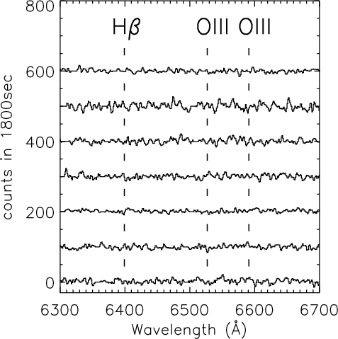 |
Figure 2:
Shown here are parts of the G600R spectra were H |
| Open with DEXTER | |
For none of the confirmed emission-line objects S7-S13 did we
detect any other emission line, neither in the G600B nor in the
G600R spectra. In Fig. 2 we
show the regions of the G600R spectra where the H![]() and O III lines would have fallen if the emission lines
seen in Fig. 1 had been O II at z=0.313 (S7
at the bottom and S13 at the top).
The spectra have been smoothed by a 7 pixel (7.4 Å) boxcar filter
and regions with large errors due to strong sky-lines were set to
zero. As seen, H
and O III lines would have fallen if the emission lines
seen in Fig. 1 had been O II at z=0.313 (S7
at the bottom and S13 at the top).
The spectra have been smoothed by a 7 pixel (7.4 Å) boxcar filter
and regions with large errors due to strong sky-lines were set to
zero. As seen, H![]() and O III lines are not
present in any of the spectra.
The question of possible alternatives to the Ly
and O III lines are not
present in any of the spectra.
The question of possible alternatives to the Ly![]() identification is an important one, and we shall return to a complete
discussion in Sect. 4.1. For now we shall assume that
the lines are indeed due to Ly
identification is an important one, and we shall return to a complete
discussion in Sect. 4.1. For now we shall assume that
the lines are indeed due to Ly![]() .
.
The wavelengths and widths of the emission lines were determined by
fitting them with Gaussian profiles. The uncertainty in the
determination of the wavelength centroid is about 0.3 Å. The
results are given in Table 2 where we also list the
resulting redshifts under the assumption that the lines are due to
Ly![]() .
.
In order to constrain the intrinsic width of the lines we must know the
spectroscopic resolution. An upper limit to the fwhm of the resolution
profile along the dispersion direction can be obtained from the
width of the slitlets and the dispersion. With a slit width of 1.2
arcsec (3 pixels) and dispersion of 2.4 Å per pixel the resolution
would have been about 7.2 Å if the seeing had been worse than 1.2
arcsec. However, as the seeing was in all cases significantly better
than 1.2 arcsec the spectroscopic resolution is smaller than 7.2 Å fwhm. An upper limit to the spectroscopic resolution can be derived from
the spatial profile of the spectra of point sources at wavelengths near
4900 Å. Converted to Å the spatial widths are 5.9 Å, 5.7 Å and
4.8 Å for maskB1, maskB2 and maskB3 respectively. As the instrumental
resolution for FORS is slightly lower along the dispersion direction
than along the spatial direction (T. Szeifert, private communication)
these values can be used as lower limits on the spectroscopic
resolution. From this lower limit we can obtain upper limits to the
intrinsic widths of the lines by deriving the intrinsic widths
that convolved with a Gaussian with a width corresponding
to the lower limit on the spectroscopic resolution reproduces the
observed line widths. These upper limits are also given in
Table 2. The line widths are smaller than 6 Å or 370 km s-1 for Ly![]() at z=3.04.
at z=3.04.
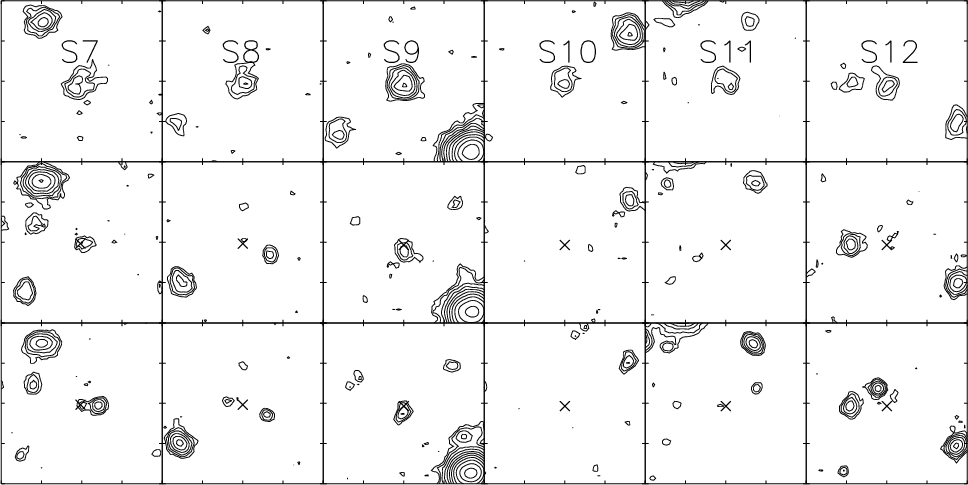 |
Figure 3:
Contour plots of the combined NTT narrow-band (top), VLT
B-band (middle) and VLT I-band (bottom) images for each of the six
candidate emission line galaxies S7-S12 detected with S/N>5 in the
NTT narrow-band image (Paper I). The size of the individual fields
is
|
| Open with DEXTER | |
Figure 3 and the two left panels in Fig. 4 show
regions of size 12![]() 12 arcsec2 centred on each of the
objects S7-S12 and S13-S14 from the combined NTT narrow-band image
(top row), VLT B-band image (middle row) and VLT
I-band image (bottom row). Only two of the objects, S7 and S9, are
detected above our 2
12 arcsec2 centred on each of the
objects S7-S12 and S13-S14 from the combined NTT narrow-band image
(top row), VLT B-band image (middle row) and VLT
I-band image (bottom row). Only two of the objects, S7 and S9, are
detected above our 2![]() detection limits of
detection limits of
![]() and
and
![]() (detection limits for 1 arcsec2 circular apertures).
Those two galaxies were already detected in the deep NTT
images presented in Paper I. For S9 both the B-band and I-band
emission is centred
(detection limits for 1 arcsec2 circular apertures).
Those two galaxies were already detected in the deep NTT
images presented in Paper I. For S9 both the B-band and I-band
emission is centred
![]() arcsec south of the narrow-band
position. In the broad band images of S7 we see two nearby objects.
The center of the Ly
arcsec south of the narrow-band
position. In the broad band images of S7 we see two nearby objects.
The center of the Ly![]() emission is found
emission is found
![]() arcsec
east of the easternmost of the two, which we identify as the likely
host of the Ly
arcsec
east of the easternmost of the two, which we identify as the likely
host of the Ly![]() emission. We cannot be certain that the
nearby western object is unrelated, hence the aperture magnitudes
for S7 given in Table 2 includes both of the objects.
The not-confirmed (
emission. We cannot be certain that the
nearby western object is unrelated, hence the aperture magnitudes
for S7 given in Table 2 includes both of the objects.
The not-confirmed (![]() )
candidate S14 is clearly detected in
both the B and I bands. The B magnitude is bright enough to confirm that
the apparent narrow-band excess in the old data set was not
significant.
)
candidate S14 is clearly detected in
both the B and I bands. The B magnitude is bright enough to confirm that
the apparent narrow-band excess in the old data set was not
significant.
For the five remaining objects we detect no broad band flux above
2![]() .
In order to constrain the limit on the broad band emission
further we registered the sub-images of the objects S8, S10-S13 to
the centroids of their Ly
.
In order to constrain the limit on the broad band emission
further we registered the sub-images of the objects S8, S10-S13 to
the centroids of their Ly![]() emission and coadded them.
In the right panel of Fig. 4 we show the median of the
coadded images. We now detect a faint object in both the I-band
and the B-band. To be able to compare the fluxes we apply aperture
corrections determined from a bright point source and arrive at
emission and coadded them.
In the right panel of Fig. 4 we show the median of the
coadded images. We now detect a faint object in both the I-band
and the B-band. To be able to compare the fluxes we apply aperture
corrections determined from a bright point source and arrive at
![]() and
and
![]() for the
3.5 arcsec diameter circular aperture.
for the
3.5 arcsec diameter circular aperture.
If this flux was due mainly to one or two of the objects, they
would have been visible on the individual images. Hence, we conclude
that the flux must be fairly evenly distributed on most or all of the
five objects, and that they each must have roughly the magnitudes measured
in the combined images. It is interesting to note that unlike S7 and S9,
the continuum emission in the coadded frames is centered on the same
position as the Ly![]() emission. This suggests that the relatively
bright continuum object identified as S9 and the two-component
object identified as S7 are, at least partly, due to a chance alignment
of unrelated objects. Hence, the broad-band magnitudes given for S7 and
S9 should probably be regarded as upper limits on their brightness.
emission. This suggests that the relatively
bright continuum object identified as S9 and the two-component
object identified as S7 are, at least partly, due to a chance alignment
of unrelated objects. Hence, the broad-band magnitudes given for S7 and
S9 should probably be regarded as upper limits on their brightness.
Møller & Warren (1998) reported that on HST images of three
Ly![]() emitting objects related to the DLA at z=2.81 in front of
PKS0528-250, there was evidence that the Ly
emitting objects related to the DLA at z=2.81 in front of
PKS0528-250, there was evidence that the Ly![]() emission was
significantly more extended than the continuum sources. We measured
the FWHM of the Ly
emission was
significantly more extended than the continuum sources. We measured
the FWHM of the Ly![]() emission of S9 and of the stacked Ly
emission of S9 and of the stacked Ly![]() object, and found an intrinsic size (after correcting for the seeing)
of 0.98 and 0.65 arcsec (FWHM). This supports the result reported
by Møller & Warren (1998).
object, and found an intrinsic size (after correcting for the seeing)
of 0.98 and 0.65 arcsec (FWHM). This supports the result reported
by Møller & Warren (1998).
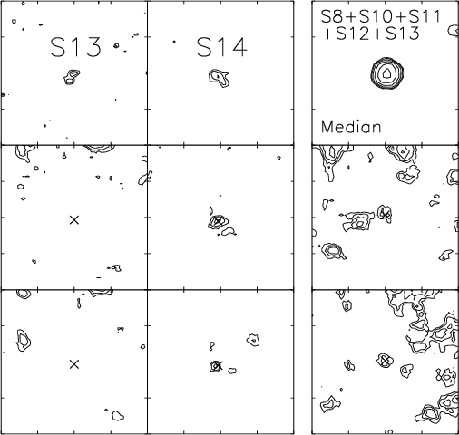 |
Figure 4:
Two left panels: Contour plots of the combined NTT
narrow-band (top), VLT
B-band (middle) and VLT I-band (bottom) images for the two
candidate emission line galaxies S13 and S14 detected with S/N<5
in the NTT narrow-band image. The size of the individual fields
is 12 |
| Open with DEXTER | |
We now return in more detail to the identification of the detected
emission lines. For a discussion of ways to discriminate between Ly![]() and lower redshift objects for single emission lines around 8000-9000 Å,
corresponding to very high redshifts (
and lower redshift objects for single emission lines around 8000-9000 Å,
corresponding to very high redshifts (
![]() )
for Ly
)
for Ly![]() ,
see
Stern et al. (2000). Here we discuss possible
contaminants for z=3 Ly
,
see
Stern et al. (2000). Here we discuss possible
contaminants for z=3 Ly![]() emitters.
emitters.
Mg II and Ne III can both be excluded easily since
in this case we would have detected the stronger O II line.
In the following we will discuss how to reject the possibility
that the observed line is due to O II.
There are two independent ways to
check the likelyhood of the identification as Ly![]() rather than
O II. One is by
its equivalent width, the other by upper limits on line flux ratios.
We shall here apply both tests, and as reference point for the low
redshift identification we have chosen the large sample of emission
line galaxies from the survey of
Terlevich et al. (1991).
rather than
O II. One is by
its equivalent width, the other by upper limits on line flux ratios.
We shall here apply both tests, and as reference point for the low
redshift identification we have chosen the large sample of emission
line galaxies from the survey of
Terlevich et al. (1991).
The continuum of low redshift O II galaxies is, in contrast to
that of the Ly![]() selected galaxies at high redshift,
for the most part easily detected. In the sample of Terlevich et al.
(1991) we find a median O II rest equivalent width of 59 Å, and
the 95% quantile is 163 Å.
In Table 2 we list the observed equivalent widths
(
selected galaxies at high redshift,
for the most part easily detected. In the sample of Terlevich et al.
(1991) we find a median O II rest equivalent width of 59 Å, and
the 95% quantile is 163 Å.
In Table 2 we list the observed equivalent widths
(
![]() )
of our lines. As discussed above, the broad-band
aperture magnitudes of the two objects S7 and S9 probably include
flux unrelated to the emission line objects, and hence the calculated
equivalent widths are lower limits. For the remaining objects it was
necessary to coadd the images before we were able to measure their
broad-band flux. For consistency we list the equivalent width measured
on the stacked images.
)
of our lines. As discussed above, the broad-band
aperture magnitudes of the two objects S7 and S9 probably include
flux unrelated to the emission line objects, and hence the calculated
equivalent widths are lower limits. For the remaining objects it was
necessary to coadd the images before we were able to measure their
broad-band flux. For consistency we list the equivalent width measured
on the stacked images.
For an O II galaxy at z=0.31 we would expect a median
equivalent width of 77 Å and none of seven objects should be above the
95% quantile of 214 Å. This is incompatible with the observed
distribution.
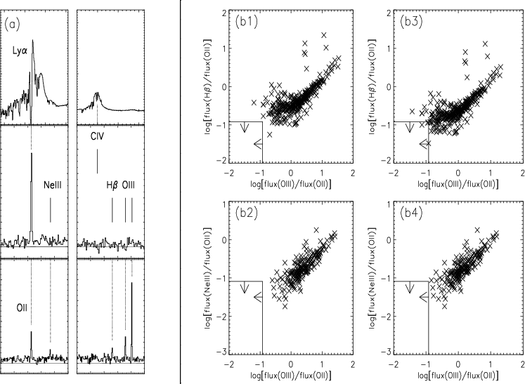 |
Figure 5:
a) Middle panel shows the stacked G600B (left) and G600R (right)
spectrum of S7-S13. Lower panel shows, for comparison, the spectrum of
a z=0.224 emission line galaxy redshifted to
z=0.313 so that the O II line falls at the wavelength of the
observed emission line of S7-S13. The stacked spectrum of
S7-S13 has none of the lines expected if S7-S13 had been foreground
emission line galaxies. Upper panel shows the spectrum of Q1205-30
to indicate the position of the C IV emission expected for AGNs.
A C IV emission line is not detected.
b) The box to the lower left of each of the figures
(b1,2,3,4) marks the 2 |
| Open with DEXTER | |
In order to compare the intensity ratios, we first had to determine
the upper limit for the non-detection of lines in the predicted
region for O III and H![]() .
For the flux calibration
of the G600R spectra we used the exact same method as described in
Sect. 3.1.1 for G600B. To maximixe the S/N for the
non-detection of H
.
For the flux calibration
of the G600R spectra we used the exact same method as described in
Sect. 3.1.1 for G600B. To maximixe the S/N for the
non-detection of H![]() and O III emission lines, we
stacked all the spectra. In Fig. 5a we show the stacked spectrum
(middle panel), and we have marked the expected positions of various
emission lines. We find 2
and O III emission lines, we
stacked all the spectra. In Fig. 5a we show the stacked spectrum
(middle panel), and we have marked the expected positions of various
emission lines. We find 2![]() upper limits to the log of flux
ratios as follows:
log(
upper limits to the log of flux
ratios as follows:
log(
![]() ,
log(
,
log(
![]() ,
and
log(
,
and
log(
![]() .
Above the stacked spectrum we plot the spectrum of the quasar
in order to show the positions of the Ly
.
Above the stacked spectrum we plot the spectrum of the quasar
in order to show the positions of the Ly![]() and C IV
emission lines. No C IV line is detected in the stacked
spectrum. The flux ratio
(log(
and C IV
emission lines. No C IV line is detected in the stacked
spectrum. The flux ratio
(log(
![]() )
excludes a significant AGN contribution to the Ly
)
excludes a significant AGN contribution to the Ly![]() emission.
Below the stacked spectrum we show for comparison the spectrum of an
O II galaxy observed by chance during the same run
in one of the slits we placed on random objects in order to fill the
masks. This galaxy was observed at a redshift of z(O II)=0.224,
but we have shifted it to z=0.313 for easy comparison.
emission.
Below the stacked spectrum we show for comparison the spectrum of an
O II galaxy observed by chance during the same run
in one of the slits we placed on random objects in order to fill the
masks. This galaxy was observed at a redshift of z(O II)=0.224,
but we have shifted it to z=0.313 for easy comparison.
In Terlevich et al. (1991) we only found data for the equivalent widths
of their emission line sample. In order to convert those to intensity
ratios of two lines, we need first to determine the ratio of the local
continuum flux under those two lines. In all the published spectra of
the Terlevich sample we therefore measured the ratio of the continuum
flux at 3727-3870 Å (OII and NeIII) and at 5007 Å (OIII). We then
determined the mean of this ratio and the maximum of the
ratio (which is the worst case), and used both of them to
convert the equivalent width ratios to flux ratios. The results are plotted
in Fig. 5b. In Figs. 5b1, b2 we plot line flux ratios calculated
from the mean continuum slope. The box and arrows in the
lower left corner marks the 2![]() upper limits of our
non-detections. In Figs. 5b3, b4 we repeat the same plots, but here
we have used the "worst case'' continuum for the conversion to flux
ratios. Even in this case our 2
upper limits of our
non-detections. In Figs. 5b3, b4 we repeat the same plots, but here
we have used the "worst case'' continuum for the conversion to flux
ratios. Even in this case our 2![]() upper limits have no overlap
with the O II galaxy distribution.
upper limits have no overlap
with the O II galaxy distribution.
In summary of this section we have applied two independent methods
(equivalent widths and line flux ratios) to test how well our sample
of emission line objects would fit if interpreted as low redshift
O II galaxies. Both tests reject the interpretation, and
we conclude that all seven objects
presented here are Ly![]() emitters at
emitters at
![]() .
.
In Paper I we calculated star-formation rates (SFR) based on the
Ly![]() fluxes. Here, for comparison, we calculate the SFRs from
the continuum fluxes. As detailed in Sect. 3.2 we have
reasons to believe that the continuum of S7 and S9 may be boosted by
neighbour objects, therefore we perform the calculation for the
remaining five objects only.
fluxes. Here, for comparison, we calculate the SFRs from
the continuum fluxes. As detailed in Sect. 3.2 we have
reasons to believe that the continuum of S7 and S9 may be boosted by
neighbour objects, therefore we perform the calculation for the
remaining five objects only.
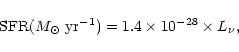
The restframe UV continuum in the range 1500 Å-2800 Å can be used as a SFR estimator if one assumes that the star-formation is
continuous over a time scale of more than 108 years. Kennicutt (1998)
provides the relation
| Survey | z, |
Area | 5 |
N |
|
field | Confirmed | Ref. |
|
|
#/
|
|||||||
| PKS0528-250 | 2.81, 0.019 | 27 | 3.7 | 3 | QSO, DLA | all | (1,2) | |
| HDF N | 3.43, 0.063 | 29 | 3.0 | 5 | blank | all, 2 AGN | (3,4) | |
| SSA 22 | 3.43, 0.063 | 30 | 1.5 | 7 | blank | all | (3,4) | |
| BR0019-152 | 3.43, 0.063 | 16 | - | 7 | blank | 3/7 | (3,4) | |
| Virgo | 3.15, 0.043 | 50 | 2.0 | 9 | blank | all | (5) | |
| SSA 22a | 3.09, 0.066 | 78 | 3.0a | 72 | LBG spike | 12/72 | (6) | |
| Q1205-30 | 3.04, 0.016 | 28 | 1.1 | 7 | QSO | all | (7) |
From the Ly![]() fluxes we found SFRs for the same objects in the
range 0.3-0.5 h-2
fluxes we found SFRs for the same objects in the
range 0.3-0.5 h-2 ![]() yr-1 for a
yr-1 for a
![]() cosmology. Converting to the cosmology used in this paper this
corresponds to 1.6-2.6
cosmology. Converting to the cosmology used in this paper this
corresponds to 1.6-2.6 ![]() yr-1, which is
identical to what we now find from the I-band flux. This result is
inconsistent with the presence of large amounts of dust in those
objects, which is not too surprising as one would expect that a
targeted search for Ly
yr-1, which is
identical to what we now find from the I-band flux. This result is
inconsistent with the presence of large amounts of dust in those
objects, which is not too surprising as one would expect that a
targeted search for Ly![]() emitters would preferentially find
objects with very little or no dust. This does however imply
that a large number of small star-forming objects at high redshift have
essentially no dust in them.
emitters would preferentially find
objects with very little or no dust. This does however imply
that a large number of small star-forming objects at high redshift have
essentially no dust in them.
The density of Ly![]() emitters derived from the seven confirmed
objects is
emitters derived from the seven confirmed
objects is ![]() per arcmin2 per unit redshift (seven objects
within the 27.6 arcmin2 field of view of the EMMI instrument of NTT
and within the
per arcmin2 per unit redshift (seven objects
within the 27.6 arcmin2 field of view of the EMMI instrument of NTT
and within the
![]() range of the narrow filter).
In Table 3 we compare this to the results from
other recent searches for LEGOs at
range of the narrow filter).
In Table 3 we compare this to the results from
other recent searches for LEGOs at ![]() .
It is seen from
Table 3 that our survey found a larger space density than
any other survey, but also that we reach the faintest detection
limit of them all. The known LBG overdensity studied by Steidel et al.
(2000) has a similar space density, but to a three times brighter
flux limit. Down to their flux limit we would only have detected two
of our seven sources. It is hence not clear from this if the volume
around Q1205-30 is overdense in LEGOs, or if we simply see the
effect of observing to a lower limiting flux. To be able to address
this question, we need to compare our results to the extrapolation
of the LBG LF.
.
It is seen from
Table 3 that our survey found a larger space density than
any other survey, but also that we reach the faintest detection
limit of them all. The known LBG overdensity studied by Steidel et al.
(2000) has a similar space density, but to a three times brighter
flux limit. Down to their flux limit we would only have detected two
of our seven sources. It is hence not clear from this if the volume
around Q1205-30 is overdense in LEGOs, or if we simply see the
effect of observing to a lower limiting flux. To be able to address
this question, we need to compare our results to the extrapolation
of the LBG LF.
Adelberger & Steidel (2000)
present a LF for LBG selected galaxies which is based
on the HDF-North for the faint (25<R<27) and ground based
LBG surveys for the bright (R<25.5) end. Integrating this
LF down to R=27 leads to a predicted density of
objects of 0.017 Mpc-3h3. The comoving volume probed by
our survey is
![]() Mpc3h-3. Based on the
LF of LBGs we therefore expect ten galaxies in the
volume and we find seven. However, only
Mpc3h-3. Based on the
LF of LBGs we therefore expect ten galaxies in the
volume and we find seven. However, only ![]() 20% of the Lyman-Break
galaxies show Ly
20% of the Lyman-Break
galaxies show Ly![]() in emission (Steidel et al. 2000). This may
be an underestimate if Ly
in emission (Steidel et al. 2000). This may
be an underestimate if Ly![]() and continuum emission in general
have different spatial distributions due to different slit-losses.
and continuum emission in general
have different spatial distributions due to different slit-losses.
With the Lyman-Break technique the only way to probe the
![]() part of the LF is to use the Hubble Deep Fields. This
makes it impossible at present to study the faint end LF of any
significant volume with this technique, and it is therefore very
uncertain. Indeed, significant differences in the numbers of high redshift
objects in the HDF North and South fields based on photometric redshifts
have been reported (Fontana et al. 2000).
The faint end of the LF is, however,
important to study because a significant fraction of the
star-formation, and therefore also the background ionising photons, may
originate there. Based on the LF of Adelberger &
Steidel (2000) there are roughly equal amounts of total luminosity from
galaxies with R<25.5, 25.5<R<27 and 27<R<30. Hence, even if
this LF is correct, only about one third of the total
star formation at z=3 is traced by the LBGs studied in the ground based
samples. In case the faint end LF needs to be revised upwards it will
be even less.
part of the LF is to use the Hubble Deep Fields. This
makes it impossible at present to study the faint end LF of any
significant volume with this technique, and it is therefore very
uncertain. Indeed, significant differences in the numbers of high redshift
objects in the HDF North and South fields based on photometric redshifts
have been reported (Fontana et al. 2000).
The faint end of the LF is, however,
important to study because a significant fraction of the
star-formation, and therefore also the background ionising photons, may
originate there. Based on the LF of Adelberger &
Steidel (2000) there are roughly equal amounts of total luminosity from
galaxies with R<25.5, 25.5<R<27 and 27<R<30. Hence, even if
this LF is correct, only about one third of the total
star formation at z=3 is traced by the LBGs studied in the ground based
samples. In case the faint end LF needs to be revised upwards it will
be even less.
Assuming for now that the 20% Ly![]() fraction can be extrapolated
to the faint end of the LF, we find that the volume we have surveyed
has a comoving density of faint LBGs which is 3.5 times that predicted
by the HDF-North LF. This could indicate that at least some radio quiet
QSOs reside in overdense environments. Another likely interpretation is,
however, that the faint end of the LF has a larger fraction of Ly
fraction can be extrapolated
to the faint end of the LF, we find that the volume we have surveyed
has a comoving density of faint LBGs which is 3.5 times that predicted
by the HDF-North LF. This could indicate that at least some radio quiet
QSOs reside in overdense environments. Another likely interpretation is,
however, that the faint end of the LF has a larger fraction of Ly![]() emitters, in our case it must be of order 70% to fit the HDF-North
LBG LF. A physical explanation could be that the objects in the
faint end of the LBG LF are less dusty that the bright LBGs.
emitters, in our case it must be of order 70% to fit the HDF-North
LBG LF. A physical explanation could be that the objects in the
faint end of the LBG LF are less dusty that the bright LBGs.
The Ly![]() emitters were selected in a deep narrow-band search. It
now remains to be tested if the objects span the entire width of the
narrow-band filter, or if they cluster within a wavelength range
smaller than the filter width. The width of the filter response was
23 Å, and the full width spanned by the seven objects is 21.2 Å.
Monte Carlo simulations, where we randomly distributed seven objects
weighted by the filter transmission curve and measured the resulting
mean and std.dev., show that the seven redshifts of S7-S13 are
consistent (to within 1
emitters were selected in a deep narrow-band search. It
now remains to be tested if the objects span the entire width of the
narrow-band filter, or if they cluster within a wavelength range
smaller than the filter width. The width of the filter response was
23 Å, and the full width spanned by the seven objects is 21.2 Å.
Monte Carlo simulations, where we randomly distributed seven objects
weighted by the filter transmission curve and measured the resulting
mean and std.dev., show that the seven redshifts of S7-S13 are
consistent (to within 1![]() )
with being drawn from a random
distribution. Therefore, the structure we have found is most likely
larger than the redshift span we have covered with our filter.
)
with being drawn from a random
distribution. Therefore, the structure we have found is most likely
larger than the redshift span we have covered with our filter.
We have reported on spectroscopic observations of eight candidate
Ly![]() emitting objects at
emitting objects at
![]() .
All six "certain''
(
.
All six "certain''
(![]() )
candidates were confirmed, and of the two "possible''
(
)
candidates were confirmed, and of the two "possible''
(![]() )
candidates one was confirmed. To assess the most likely
identification of the lines we performed two independent detailed
tests based on a large sample of low redshift O II galaxies.
Both tests indicate that the only likely identification is Ly
)
candidates one was confirmed. To assess the most likely
identification of the lines we performed two independent detailed
tests based on a large sample of low redshift O II galaxies.
Both tests indicate that the only likely identification is Ly![]() .
This conclusion is strengthened by the fact that the original
narrow-band imaging was centered on a quasar at the same redshift.
The seven Ly
.
This conclusion is strengthened by the fact that the original
narrow-band imaging was centered on a quasar at the same redshift.
The seven Ly![]() objects are hence likely associated with the same
structure as the quasar.
objects are hence likely associated with the same
structure as the quasar.
The narrow-band images of the objects, as well as the large
slit-losses of Ly![]() emission
we need to correct for when calibrating the line fluxes,
indicate that the Ly
emission
we need to correct for when calibrating the line fluxes,
indicate that the Ly![]() emission originates in extended objects.
This is similar to the results reported by Møller & Warren (1998)
on Ly
emission originates in extended objects.
This is similar to the results reported by Møller & Warren (1998)
on Ly![]() emission related to a DLA at z=2.81, where it was found
that the Ly
emission related to a DLA at z=2.81, where it was found
that the Ly![]() emission was significantly more extended than the
continuum sources. As these authors point out, this could cause a severe
underestimate of the Ly
emission was significantly more extended than the
continuum sources. As these authors point out, this could cause a severe
underestimate of the Ly![]() equivalent widths measured on spectra
of high redshift galaxies obtained through a slit.
equivalent widths measured on spectra
of high redshift galaxies obtained through a slit.
An analysis of the redshift distribution of the seven confirmed
Ly![]() objects shows that it is consistent with a random
distribution in the redshift interval selected via the narrow-band
filter.
objects shows that it is consistent with a random
distribution in the redshift interval selected via the narrow-band
filter.
Despite deep detection limits only S7 and S9 were detected
directly in the combined B and I band images. For S8 and
S10-S13 we registered the broad band images using the
positions of the Ly![]() sources and determined the
median image of the five. This procedure allowed the detection
of broad band emission at the level of
sources and determined the
median image of the five. This procedure allowed the detection
of broad band emission at the level of
![]() and
and
![]() respectively. This means that S8 and
S10-S13 belong to the faint end of the LF at z=3.
The derived space density of LEGOs is consistent
with the integrated LF of LBGs down to R=27. However,
only about 20% of R<25.5 LBGs are Ly
respectively. This means that S8 and
S10-S13 belong to the faint end of the LF at z=3.
The derived space density of LEGOs is consistent
with the integrated LF of LBGs down to R=27. However,
only about 20% of R<25.5 LBGs are Ly![]() emitters
(Steidel et al. 2000).
Hence, either the fraction of Ly
emitters
(Steidel et al. 2000).
Hence, either the fraction of Ly![]() emitters at the faint
end of the LF is significantly higher than 20%
or the space density of galaxies in the field of Q1205-30
is higher than predicted by the LBG LF. The latter would
indicate that at least some radio quiet QSOs at high redshift
reside in overdense environments.
emitters at the faint
end of the LF is significantly higher than 20%
or the space density of galaxies in the field of Q1205-30
is higher than predicted by the LBG LF. The latter would
indicate that at least some radio quiet QSOs at high redshift
reside in overdense environments.
It has long been argued that Ly![]() based searches for high
redshift galaxies were doomed to failure, because even a small amount
of dust would quench the Ly
based searches for high
redshift galaxies were doomed to failure, because even a small amount
of dust would quench the Ly![]() emission due to the resonant
scattering of the Ly
emission due to the resonant
scattering of the Ly![]() photons. For this reason it has been
virtually impossible to obtain telescope time for Ly
photons. For this reason it has been
virtually impossible to obtain telescope time for Ly![]() survey
work. We note here in passing that the recent very successful Ly
survey
work. We note here in passing that the recent very successful Ly![]() survey by Kudritzki et al. (2000) was aimed at low redshift planetary
nebulae, and the work
that supplied our candidate list was aimed at the imaging of a
quasar absorber. It is virtually certain that neither of those
programmes had been granted telescope time if the aim had been to
search for a sample of Ly
survey by Kudritzki et al. (2000) was aimed at low redshift planetary
nebulae, and the work
that supplied our candidate list was aimed at the imaging of a
quasar absorber. It is virtually certain that neither of those
programmes had been granted telescope time if the aim had been to
search for a sample of Ly![]() emitters at z=3.
emitters at z=3.
In this paper we find two strong arguments against the presence of
significant amounts of dust in the objects in the faint end of the
high redshift galaxy LF. Firstly we find very large equivalent widths,
in the upper range of theoretical predictions. Secondly we find that
when we calculate the star-formation rate from the continuum flux and
from the Ly![]() flux independently, we obtain identical results.
Both of those observations are inconsistent with a dust-rich
environment.
flux independently, we obtain identical results.
Both of those observations are inconsistent with a dust-rich
environment.
The faint continuum magnitudes detected for S8 and S10-S13
prove that Ly![]() emission is a powerful method by which to probe
the faint end of the galaxy LF at
emission is a powerful method by which to probe
the faint end of the galaxy LF at ![]() .
The next step is now to obtain statisitically significant samples,
containing several hundred Ly
.
The next step is now to obtain statisitically significant samples,
containing several hundred Ly![]() selected galaxies,
in order to further constrain the properties of the faint end of the
luminosity function.
selected galaxies,
in order to further constrain the properties of the faint end of the
luminosity function.
Acknowledgements
We are grateful for excellent support during our service observations in January and during the observing run on Paranal in March. We thank the referee A. Fontana for several comments that clarified our manuscript on important points.