1 - Stockholm Observatory, 133 36 Saltsjöbaden, Sweden
2 - European Southern Observatory, Karl-Schwarzschild-Strasse 2, 85748 Garching bei München, Germany

Abstract
ISO/SWS observations of SN 1987A on day 3425 show no emission in [Fe I] 24.05 $\mu {\rm m}$ and [Fe II] 25.99 $\mu {\rm m}$ down to the limits $\sim$ 0.39 Jy and $\sim$ 0.64 Jy, respectively. Assuming a homogeneous distribution of ⁴⁴Ti inside $2000 {\rm ~km~s^{-1}}$ and negligible dust cooling, we have made time dependent theoretical models to estimate an upper limit on the mass of ejected ⁴⁴Ti. Assessing various uncertainties of the model, and checking the late optical emission it predicts, we obtain an upper limit of $\simeq$ $1.1\times 10^{-4}~{M}_\odot$ . This is lower than in our previous estimate using other ISO data, and we compare our new result with other models for the late emission, as well as with expected yields from explosion models. We also show that steady-state models for the optical emission are likely to overestimate the mass of ejected ⁴⁴Ti. The low limit we find for the mass of ejected ⁴⁴Ti could be higher if dust cooling is important. A direct check on this is provided by the gamma-ray emission at 1.157 Mev as a result of the radioactive decay of ⁴⁴Ti.

Key words: supernova: individual: SN 1987A - nucleosynthesis - supernovae: general

While $M(^{56}{\rm Ni})$ and $M(^{57}{\rm Ni})$ are rather accurately known for SN 1987A, with $M(^{56}{\rm Ni}) \approx 0.071 ~{M}_\odot$ (e.g., Suntzeff & Bouchet 1990), and $M(^{57}{\rm Ni}) \sim 3.3\times 10^{-3} ~{M}_\odot$ (Fransson & Kozma 1993, and references therein), the situation is more uncertain for ⁴⁴Ti. To some extent this has been due to a poorly known decay time of this isotope, although this has recently improved; ⁴⁴Ti decays first to ⁴⁴Sc, on a time scale of $87.0\pm1.9$ years (Ahmad et al. 1998; Görres et al. 1998; see also Norman et al. 1998 who obtain $86\pm3$ years), and then quickly further to ⁴⁴Ca.

Based on time dependent modeling, K00 estimates that ${M(^{44}{\rm Ti})} = (1.5 \pm 1.0) \times 10^{-4} ~{M}_\odot$ best explains the evolution of the optical broad-band photometry of SN 1987A for $t \!\!\!\phantom{\le}\smash{\buildrel{}\over {\lower2.5dd\hbox{$\buildrel{\lower2dd\hbox{$\displaystyle<$ }}\over \sim$ }}}\,\,3270$ days. This is consistent with Chugai et al. (1997), who find ${M(^{44}{\rm Ti})} \sim (1$ - $2)\times 10^{-4} ~{M}_\odot$ from the optical line emission at 2875 days, and Mochizuki & Kumagai (1998) who obtain the same result from a light curve analysis (see also Nagataki 2000). However, as is shown by K00, both broad-band photometry and the emission modeled by Chugai et al. (1997) constitute only a minor fraction of the total emission put out by the supernova. At these epochs most of the emission from the supernova instead comes out in the far infrared (IR) in a few iron lines, most notably [Fe II] 25.99 $\mu {\rm m}$ . This makes bolometric corrections to the late optical data rather uncertain, and a more direct way to measure the content of ${M(^{44}{\rm Ti})}$ is to measure the flux in the far-IR lines.

In a recent study Lundqvist et al. (1999; henceforth L99) analyze Infrared Space Observatory (ISO; Kessler et al. 1996) data obtained mainly at t = 3999 days. L99 couple these observations to time dependent model calculations similar to those in K00, and from the absence of iron line emission in the ISO spectra they derive ${M(^{44}{\rm Ti})} \!\!\!\phantom{\le}\smash{\buildrel{}\over {\lower2.5dd\hbo... ...wer2dd\hbox{$\displaystyle<$ }}\over \sim$ }}}\,\,1.5\times 10^{-4} ~{M}_\odot$ . This limit is consistent with the results of Chugai et al. (1997), Mochizuki & Kumagai (1998) and K00. A different limit was obtained by Borkowski et al. (1997) who in their preliminary analysis of ISO data from t = 3425 days derive ${M(^{44}{\rm Ti})} \!\!\!\phantom{\le}\smash{\buildrel{}\over {\lower2.5dd\hbo... ...wer2dd\hbox{$\displaystyle<$ }}\over \sim$ }}}\,\,1.5\times 10^{-5} ~{M}_\odot$ . Such a low titanium mass would have important consequences for models of the explosion. Here we analyze the data of Borkowski et al. in the same way as was done for the 3999 day data in L99, however, expanding the discussion on the uncertainties of our method. In particular, we discuss the uncertainty of the temperature, which is important since the far-IR lines are collisionally excited, and their excitation energy (e.g., $T \approx 550$ K for the 26 $\mu {\rm m}$ line) is much higher than the gas temperature. Because the emission at this epoch is powered mainly by positrons from the decay of ⁴⁴Ti, we also discuss the uncertainty of the line fluxes due to the efficiency of the trapping of positrons.

2 Observations and results

We have used the ISO data discussed in Borkowski et al. (1997). These data were obtained on 10 July, 1996 (i.e., on day 3425 of SN 1987A) in the SWS06 mode of the Short Wavelength Spectrograph (SWS; de Graauw et al. 1996). The data we analyze span the regions $23.59 {-} 25.04~\mu{\rm m}$ and $25.51 {-} 26.53~\mu{\rm m}$ . Both these ranges are covered by band 3D of SWS, and include the lines [Fe I] 24.05 $\mu {\rm m}$ and [Fe II] 25.99 $\mu {\rm m}$ , i.e., the two strongest lines expected from the supernova (cf. L99). These data are superior to those discussed in L99 as the SWS06 scans are deeper than the SWS01 scans in L99, and include a large enough wavelength interval for accurate continuum determination compared to the SWS02 data in L99.

The data were retrieved from the ISO archive, and have been reduced with the off-line processing (OLP/pipeline) version 8.7. We used ISO Spectral Analysis Package (ISAP) to flatfield and average over the scan directions. The averaging over the detectors was done with a resolution of R = 300, using the standard $2.5\sigma$ -clipping.

$\begin{figure} \par\includegraphics[angle=0, width=8.8cm]{H2730F1.PS}\end{figure}$

Figure 1: ISO SWS/AOT6 spectra of SN 1987A on day 3425. The spectra were reduced using the pipeline software (see text). The bin size is $\approx$ 0.081 (0.086) $~\mu{\rm m}$ for [Fe I] 24.05 $\mu {\rm m}$ ([Fe II] 25.99 $\mu {\rm m}$ ) (see text), which is low enough compared to the expected line width. Overlaid (dashed lines) are the line emissions from a model with ${M(^{44}{\rm Ti})} = 5\times 10^{-5} ~{M}_\odot$ (without photoionization) described in Table 1 and Sect. 3.2. To obtain the modeled line profiles we have assumed a maximum core velocity of $2000 {\rm ~km~s^{-1}}$ , and a homogeneously distributed emission throughout the core (see Sect. 3.2). The peak flux of [Fe II] 25.99 $\mu {\rm m}$ for this model is slightly less than what is needed for a 3 $\sigma$ detection (cf. Sect. 3.3).

Open with DEXTER

In Fig. 1 we present fully reduced spectra of SN 1987A for the two wavelength regions. Although the nominal instrumental resolution of the SWS spectra is $R~\approx 1800$ we have averaged the spectra with a bin size of R = 300, corresponding to $\approx$ $1000 {\rm ~km~s^{-1}}$ . This is sufficient to resolve the lines since they could extend to well over $2000 {\rm ~km~s^{-1}}$ . However, we detected neither [Fe I] 24.05 $\mu {\rm m}$ nor [Fe II] 25.99 $\mu {\rm m}$ in the spectra. We estimated the rms in the data with a zero-order baseline fit in the regions 23.80-24.80 $\mu {\rm m}$ and 25.60-26.40 $\mu {\rm m}$ , and found 0.11 Jy and 0.19 Jy, respectively.

The exact rms-values vary somewhat with the bin size used in the averaging routine. Reducing the bin size to R = 500 gives the limits 0.13 Jy and 0.21 Jy, respectively. In order to derive a conservative limit on the ⁴⁴Ti mass we have adopted these values. A 3 $\sigma$ limit for the $26~\mu{\rm m}$ line then becomes $\sim$ 0.64 Jy, while for the $24~\mu{\rm m}$ line it is lower, $\sim$ 0.39 Jy. The bin size is small enough so that we can use the limits for the peak of the expected line profiles in our estimate of the ⁴⁴Ti mass.

3 Interpreting the SWS observations

3.1 The model for line emission from the supernova

The thermal and ionization balances are solved time-dependently, as are also the level populations of the most important ions. A total of $\sim$ 6400 lines are included in the calculations. The radioactive isoptopes included are ⁵⁶Ni, ⁵⁷Ni, and ⁴⁴Ti, and we calculate the energy deposition of gamma-rays and positrons solving the Spencer-Fano equation (see Kozma & Fransson 1992). We assume that the positrons deposit their energy locally.

We include $0.07 ~{M}_\odot$ of ⁵⁶Ni and $3.33\times 10^{-3} ~{M}_\odot$ of ⁵⁷Ni (Sect. 1). In L99 three values of ${M(^{44}{\rm Ti})}$ were tested: ${M(^{44}{\rm Ti})} =0.5\times 10^{-4}, 1.0\times 10^{-4}$ and $2.0\times 10^{-4} ~{M}_\odot$ . Here we extend this to include three new values: ${M(^{44}{\rm Ti})} = 1.0\times 10^{-5}, 1.7\times 10^{-5}$ and $3.0\times 10^{-5} ~{M}_\odot$ . Although we follow the complete evolution of the supernova after 150 days, we concentrate our discussion mainly on 3425 and 3999 days, i.e., the epochs of the ISO observations.

In L99 an e-folding time of 78 years was used for ⁴⁴Ti, as this was thought to represent a mean value from experiments. More accurate measurements of the decay time (Ahmad et al. 1998; Görres et al. 1998; Norman et al. 1998) became available while the analysis of L99 was completed, and the results of L99 were corrected accordingly before publishing. Here, we use the more accurate e-folding time ( $87.0\pm1.9$ years) from the outset.

The explosion model we use is the same as in L99 and Kozma & Fransson (1998a). That is, we take the abundances from the 10H model (Woosley & Weaver 1986; Woosley 1988), but distribute the elements so that hydrogen is mixed into the core. Spherically symmetric geometry is assumed, and the iron-rich core extends out to $2000 {\rm ~km~s^{-1}}$ , outside of which (out to $6000 {\rm ~km~s^{-1}}$ ) a hydrogen envelope is attached.

We use the Sobolev approximation for the line transfer. This is a good approximation for well-separated lines in an expanding medium, but is poorer when lines overlap. This is actually the case in the UV, especially at earlier epochs. The overlap leads to UV-scattering which affects the UV-field within the ejecta. As in L99, we have studied two extreme cases to test this effect: photoionization as in the original model, and simply switching off the photoionization caused by the UV-field. From the results of L99 we, however, do not expect the UV-field to be the dominant source of uncertainty in our models. Another drawback of the Sobolev approximation is that we do not account for line fluorescence in which UV lines are split into optical and IR lines. To treat this accurately is beyond the scope of this paper, but is treated in detail in a forthcoming paper.

Since L99 we have updated the collision strengths for the [Fe II] $26~\mu{\rm m}$ transition. The collision strength, $\Omega$ , is given by Zhang & Pradhan (1995) as a function of temperature. The value of $\Omega$ at $T \leq 200$ K is set to $\Omega = 7.0$ (A. Pradhan, private communication). We note, however, that there can still be uncertainty in this result as a fully relativistic calculation is needed to accurately calculate the collision strength at these low temperatures (M. Bautista, private communication).

3.2 Model calculations

Table 1: Modeled line flux at 3425 days^a.

${M(^{44}{\rm Ti})}$ ( $~{M}_\odot$ )
Photoion.^b $f_{24\mu{\rm m}}$ (Jy) $f_{26\mu{\rm m}}$ (Jy)

$1.0\times 10^{-5}$
yes 0.047 0.095

$1.0\times 10^{-5}$ no 0.051 0.074

$1.7\times 10^{-5}$ yes 0.072 0.17

$1.7\times 10^{-5}$ no 0.079 0.14

$3.0\times 10^{-5}$ yes 0.11 0.34

$3.0\times 10^{-5}$ no 0.12 0.29

$5.0\times 10^{-5}$ yes 0.17 0.61

$5.0\times 10^{-5}$ no 0.18 0.53

$1.0\times 10^{-4}$ yes 0.26 1.37

$1.0\times 10^{-4}$ no 0.31 1.18

$2.0\times 10^{-4}$ yes 0.40 2.96

$2.0\times 10^{-4}$ no 0.54 2.53

^a Distance = 50 kpc. Homogeneous distribution of emitting gas inside $\pm 2000 {\rm ~km~s^{-1}}$ has been assumed.
The resulting shape of the line profile is seen Fig. 1. The flux values are the peak values of the lines assuming this profile.
^b Indicates whether or not photoionization has been included in the calculation. (See Sect. 3.1).

**Table 1:** Modeled line flux at 3425 days^a.
${M(^{44}{\rm Ti})}$ ( $~{M}_\odot$ )	Photoion.^b	$f_{24\mu{\rm m}}$ (Jy)	$f_{26\mu{\rm m}}$ (Jy)
$1.0\times 10^{-5}$	yes	0.047	0.095
$1.0\times 10^{-5}$	no	0.051	0.074
$1.7\times 10^{-5}$	yes	0.072	0.17
$1.7\times 10^{-5}$	no	0.079	0.14
$3.0\times 10^{-5}$	yes	0.11	0.34
$3.0\times 10^{-5}$	no	0.12	0.29
$5.0\times 10^{-5}$	yes	0.17	0.61
$5.0\times 10^{-5}$	no	0.18	0.53
$1.0\times 10^{-4}$	yes	0.26	1.37
$1.0\times 10^{-4}$	no	0.31	1.18
$2.0\times 10^{-4}$	yes	0.40	2.96
$2.0\times 10^{-4}$	no	0.54	2.53

The line fluxes in Table 1 are for a distance to the supernova of 50 kpc, and assuming a homogeneous distribution of emitting gas inside $\pm 2000 {\rm ~km~s^{-1}}$ . The FWHM velocity for the resulting profile (shown in Fig. 1) is $v_{\it FWHM} = 2828 {\rm ~km~s^{-1}}$ , which is close to what Haas et al. (1990) observed for [Fe II] 17.94 $\mu {\rm m}$ at $\sim$ 400 days after the explosion, $v_{\it FWHM} = (2900 \pm 80) {\rm ~km~s^{-1}}$ .

$\begin{figure} \par\includegraphics{H2730F2.PS}\par\end{figure}$

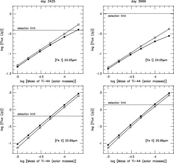Figure 1: Modeled fluxes of [Fe I] 24.05 $\mu {\rm m}$ and [Fe II] 25.99 $\mu {\rm m}$ from SN 1987A as functions of the mass of ejected ⁴⁴Ti, 3425 and 3999 days after explosion. Models with photoionization included (see text) are shown by filled squares and joined by solid lines, while for the others photoionization was not included. The inferred $3\sigma$ detection limits for the two epochs are shown as dashed-dotted lines. Note the near constancy of the modeled fluxes between the two epochs, and the rather small uncertainty due to photoionization.

Open with DEXTER

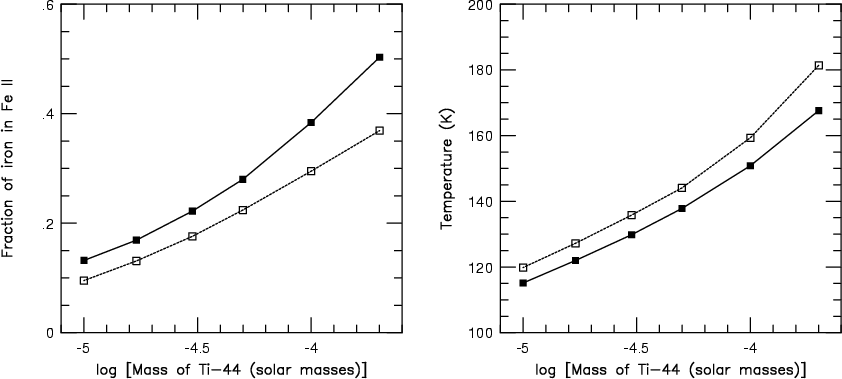$\begin{figure} \par\includegraphics{H2730F3.PS}\end{figure}$	Figure 2: Fraction of iron in Fe II, $X_{\rm FeII}$ , and temperature in the iron-rich part of the ejecta of SN 1987A at 3425 days as a function of mass of ⁴⁴Ti. Symbols and lines have the same meaning as in Fig. 2. As expected, the temperature and $X_{\rm FeII}$ increase monotonically with increasing mass of ⁴⁴Ti.
Open with DEXTER

In L99 it was discussed how the fluxes in [Fe I] 24.05 $\mu {\rm m}$ and [Fe II] 25.99 $\mu {\rm m}$ ( $f_{24\mu{\rm m}}$ and $f_{26\mu{\rm m}}$ , respectively) scale with increasing values for ${M(^{44}{\rm Ti})}$ at a given epoch. It was found that $f_{26\mu{\rm m}}$ scales nearly linearly with ${M(^{44}{\rm Ti})}$ , while $f_{24\mu{\rm m}}$ has a weaker dependence. The stronger dependence for $f_{26\mu{\rm m}}$ is due to an ionization effect because $X_{\rm FeII}$ , the relative fraction of iron in Fe II in the iron-rich gas, increases with increasing ${M(^{44}{\rm Ti})}$ . We find that this trend continues also for ${M(^{44}{\rm Ti})} < 5\times 10^{-5} ~{M}_\odot$ . This is shown in Figs. 2 and 3, where models joined by dashed (solid) lines are without (with) photoionization. Whereas $X_{\rm FeII}$ and the temperature in the iron-rich gas are only shown for 3425 days (Fig. 3), results for the line fluxes (Fig. 2) are shown for both 3425 and 3999 days. Note how the fluxes remain nearly constant between these two epochs, especially in the case of $f_{26\mu{\rm m}}$ .

The only deviation from a linear log( ${M(^{44}{\rm Ti})}$ ) versus log(f) behavior in Fig. 2 is for $f_{24\mu{\rm m}}$ at the highest values of ${M(^{44}{\rm Ti})}$ in the models with photoionization. This is because here $X_{\rm FeI}$ (the fraction of iron in Fe I in the iron-rich gas) starts to fall significantly below unity (cf. Fig. 3): for ${M(^{44}{\rm Ti})} = 0.3,(0.5),(1.0),(2.0)\times 10^{-4} ~{M}_\odot$ , $X_{\rm FeI} \approx 0.78, (0.70),(0.58),(0.44)$ at 3425 days. (The same number for the case without photoionization is $X_{\rm FeI} \approx 0.82, [0.76],[0.68],[0.58]$ .) The temperature increases monotonically with ${M(^{44}{\rm Ti})}$ (Fig. 3) and affects $f_{24\mu{\rm m}}$ and $f_{26\mu{\rm m}}$ in the same way. This is because the two lines have nearly the same excitation energy, and their effective collision strengths vary only weakly (and in our models are assumed to be constant over the small temperature regime [ $\sim$ 115-180 K] found in the iron-rich gas in our models).

Table 1 and Fig. 2 show that the 26 $\mu {\rm m}$ line is stronger than the 24 $\mu {\rm m}$ line even for the models with the lowest values of ${M(^{44}{\rm Ti})}$ (and thus the highest values of $X_{\rm FeI}$ ). This is because the collision strength for [Fe II] 25.99 $\mu {\rm m}$ line is much larger than for [Fe I] 24.05 $\mu {\rm m}$ .

Table 1 and Fig. 2 also show that switching off photoionization does not have a dramatic effect on the line fluxes. Again, the largest difference for the fluxes is for the 24 $\mu {\rm m}$ line and at the highest ${M(^{44}{\rm Ti})}$ considered. For values $\leq 5.0\times 10^{-5} ~{M}_\odot$ , switching off photoionization only affects $f_{24\mu{\rm m}}$ ( $f_{26\mu{\rm m}}$ ) by $\!\!\!\phantom{\le}\smash{\buildrel{}\over {\lower2.5dd\hbox{$\buildrel{\lower2dd\hbox{$\displaystyle<$ }}\over \sim$ }}}\,\,\!\!$ 11% ( $\!\!\!\!\!\phantom{\le}\smash{\buildrel{}\over {\lower2.5dd\hbox{$\buildrel{\lower2dd\hbox{$\displaystyle<$ }}\over \sim$ }}}\,\,\!\!$ 22%) at 3425 days. The small difference is simply due to the minor shift in the degree of ionization, from Fe II to Fe I, when photoionization is switched off.

3.3 Mass of $^\mathsfsl{44}$ Ti from [Fe II] 25.99 $\mu$ m

With the results in Fig. 2 it is straightforward to estimate the upper limit on ${M(^{44}{\rm Ti})}$ . It is clear that the best estimate within the framework of our modeling comes from the 26 $\mu {\rm m}$ line on day 3425. Using $f_{26 \mu{\rm m}} \!\!\!\phantom{\le}\smash{\buildrel{}\over {\lower2.5dd\hbox{$\buildrel{\lower2dd\hbox{$\displaystyle<$ }}\over \sim$ }}}\,\,0.64$ Jy from Sect. 2.1, we find the upper limit ${M(^{44}{\rm Ti})} \!\!\!\phantom{\le}\smash{\buildrel{}\over {\lower2.5dd\hbo... ...hbox{$\displaystyle<$ }}\over \sim$ }}}\,\,5.2~(5.9) \times 10^{-5} ~{M}_\odot$ with (without) photoionization included. A conservative limit (i.e., the case when photoionization is unimportant) is therefore ${M(^{44}{\rm Ti})} \!\!\!\phantom{\le}\smash{\buildrel{}\over {\lower2.5dd\hbo... ...er2dd\hbox{$\displaystyle<$ }}\over \sim$ }}}\,\,5.9 \times 10^{-5} ~{M}_\odot$ . In Fig. 1 we have included the expected line emission for a model with ${M(^{44}{\rm Ti})} = 5.0 \times 10^{-5} ~{M}_\odot$ , i.e., close to this limiting mass. Although our limit is nearly a factor of four higher than that found by Borkowski et al. (1997), using the same data, it is still substantially lower than found by L99 from day 3999. Using our updated code, the day 3999 data only set a limit ${M(^{44}{\rm Ti})} \!\!\!\phantom{\le}\smash{\buildrel{}\over {\lower2.5dd\hbo... ...er2dd\hbox{$\displaystyle<$ }}\over \sim$ }}}\,\,1.1 \times 10^{-4} ~{M}_\odot$ . This is a factor $\sim$ 1.7 better than can be obtained from the 24 $\mu {\rm m}$ line on day 3425. We will evaluate our limit from the 26 $\mu {\rm m}$ line on day 3425 in Sect. 4.1.

4 Discussion

4.1 Uncertainties in the modeling

A source of uncertainty, not investigated in L99, is the rather unknown rates of charge transfer for the elements in the core. In the models in Sect. 3, no charge transfer was included between Fe and excited states of He, as well as between atoms and ions of Fe. We have tested the importance of including this charge transfer, using the rates suggested by Liu et al. (1998) in a model with ${M(^{44}{\rm Ti})} \sim 1.0 \times 10^{-4} ~{M}_\odot$ and no photoionization. Compared to the model with the same ${M(^{44}{\rm Ti})}$ in Sect. 3, the model with the full charge transfer has a higher value of $X_{\rm FeII}$ by $\sim$ 20%, mainly due to charge transfer between Fe I and Fe III. However, the temperature in the model with full charge transfer is somewhat lower, so the difference in $f_{26\mu{\rm m}}$ between the two models is only $\sim$ 7%. With full charge transfer included, the estimated ${M(^{44}{\rm Ti})}$ would therefore be lower than in Sect. 3, but due to the uncertainty of the charge transfer rates, and in order to derive a conservative limit on ${M(^{44}{\rm Ti})}$ , we assign a generous error of 10% in ${M(^{44}{\rm Ti})}$ due to this effect.

L99 studied the uncertainty of the collision strength of the 26 $\mu {\rm m}$ line. Although we are now using a better fit to the results of Zhang & Pradhan (1995), the collision strength at very low temperatures is still uncertain (see Sect. 3.1). In L99 we assumed an uncertainty of $15\%$ in ${M(^{44}{\rm Ti})}$ due to this, and we retain this number also here.

The collisional excitation of the 24 $\mu {\rm m}$ and 26 $\mu {\rm m}$ lines is more sensitive to the temperature (through the ${\rm exp}(-h c/\lambda k T)$ term) than to the collision strength. Too high a temperature in our models could therefore overestimate the flux in these lines, and we would consequently underestimate ${M(^{44}{\rm Ti})}$ . We can check this effect by studying Table 1 where we see that models with ${M(^{44}{\rm Ti})} = 5.0 \times 10^{-5} ~{M}_\odot$ and ${M(^{44}{\rm Ti})} = 1.0 \times 10^{-4} ~{M}_\odot$ differ in $f_{26\mu{\rm m}}$ by a factor of $\sim$ 2.2 at 3425 days. Because the temperature in the ${M(^{44}{\rm Ti})} = 1.0 \times 10^{-4} ~{M}_\odot$ model is $\approx$ 159 K (see Fig. 3), a lowering of the temperature by only $\sim$ 20% would decrease $f_{26\mu{\rm m}}$ to the same level as in the ${M(^{44}{\rm Ti})} = 5.0 \times 10^{-5} ~{M}_\odot$ model, for constant $X_{\rm FeII}$ . However, the temperatures in our models are not free parameters but are fixed by the heating and cooling. The energy not coming out in the 24 $\mu {\rm m}$ and 26 $\mu {\rm m}$ lines must instead come out in other lines (like the optical/IR recombination lines) which are less sensitive to temperature, or as emission from dust. We will make a consistency check of the optical and far-IR emission in our models in Sect. 4.2, but we note already here that only a small transfer of energy loss from the far-IR lines to the optical/IR recombination lines would increase the optical and IR flux considerably, and then the models of K00 for the optical would severely overestimate ${M(^{44}{\rm Ti})}$ . We therefore believe we are not making a serious error in the derivation of the temperature in our models.

Dust emits a continuum which is difficult to detect, but we may for simplicity assume that the dust emission does not interact with the gas. In that case, dust cooling has exactly the same effect for the 24 $\mu {\rm m}$ and 26 $\mu {\rm m}$ line fluxes as just lowering ${M(^{44}{\rm Ti})}$ . (See the models in Sect. 3.) It may therefore well be that dust cooling could tap the supernova of its [Fe II] 25.99 $\mu {\rm m}$ emission, but it is likely that it would do so in a way which would also make the optical and near-IR lines too weak. We do not assign an explicit error in the estimated ${M(^{44}{\rm Ti})}$ due to dust cooling. (See also Sect. 4.2.)

L99 discussed uncertainties in the modeled line fluxes due to the explosion model used. As in L99 we have used the 10H explosion model (Woosley & Weaver 1986; Woosley 1988), mixed by Kozma & Fransson (1998ab) to give good agreement between their modeling and late time observations. Kozma & Fransson (1998b) compared the results from this model with a similarly mixed version of the 11E1 model (Shigeyama et al. 1988), and found that the iron lines are insensitive to the explosion model used. This is because the iron core mass, which is fixed by the amount of ejected ⁵⁶Ni, is the same in both models. We follow L99 and assign a $15\%$ error in ${M(^{44}{\rm Ti})}$ due to the choice of explosion model.

In our calculations we have assumed a local deposition of positron energy from the radioactive decay of ⁴⁴Ti. This assumption was also used in L99. The argument is that the efficiency of trapping cannot change substantially until day $\sim$ 3600 (K00), and that the most straightforward interpretation of a near-constant efficiency of trapping over an extended period of time is to assume full trapping. L99 assumed a $15\%$ error in ${M(^{44}{\rm Ti})}$ due to the uncertainty of trapping. Here we do not infer an explicit error to the models in Sect. 3, but in Sect. 4.2 we investigate this in greater detail in terms of a consistency check of the modeled IR and optical fluxes. The positron deposition is discussed in Sect. 4.2 in conjunction with clumping. Even without positron leakage, clumping of the iron-rich gas could cause an error in the estimate of ${M(^{44}{\rm Ti})}$ . However, according to L99, this error is likely to be small, $\sim$ 5%, and can be ignored when compared to other errors discussed above.

The combined error of $f_{26\mu{\rm m}}$ due to model approximations, except for different clumping and positron leakage scenarios (which will be discussed in Sect. 4.2) is therefore $\sim$ 36%. With the line profile used in Fig. 2 we thus arrive at an upper limit on ${M(^{44}{\rm Ti})}$ which is $\sim$ $8 \times 10^{-5} ~{M}_\odot$ .

4.2 Consistency check of the modeled optical and infrared emission

Although the limit on ${M(^{44}{\rm Ti})}$ we found above in Sect. 4.1 is a factor of $\sim$ 2 lower than the limit found by L99 for the 3999 data, it is still compatible with K00 (see Sect. 1). However, the agreement is not perfect although the same computer code has been used. Here we make a consistency check of the modeled optical and IR emission produced by our model. For the late optical photometry (day 3268) we adopt the same data as used by K00 (Soderberg et al. 1999). The observational error of these is approximately $\pm 0.05$ magnitudes, as judged from the systematic error in the zero point of HST/WFPC2 photometry (Mould et al. 2000; P. Challis 2000, private communcation). We have concentrated our consistency check on models with ${M(^{44}{\rm Ti})} = 10^{-4} ~{M}_\odot$ . This is close to the upper limit found in Sect. 4.1 from the far-IR lines when the errors have been considered. This value of ${M(^{44}{\rm Ti})}$ is also in the lower range of the preferred values found by K00 in her modeling of the optical and near-IR emission. This can be seen from Table 2 where the modeled V, R and I magnitudes in model M1 are all slightly fainter, by roughly half a magnitude, than the observed, while the predicted [Fe II] 26 $\mu {\rm m}$ line emission is somewhat too strong to be accommodated by our error analysis in Sect. 4.1. (Model M1 is identical to the model with ${M(^{44}{\rm Ti})} = 10^{-4} ~{M}_\odot$ and no photoionization in Table 1.)

It is obvious that our models contain simplifications that can make us systematically overproduce far-IR emission at the expense of optical emission. We still have to explore fluorescence (see Sect. 3.1), and other simplifications could be clumping and different scenarios for the deposition of positron energy. These two effects are probably also coupled. In Sect. 4.1 we mentioned that L99 found that the estimated error in ${M(^{44}{\rm Ti})}$ due to clumping alone should be small. This is true if one looks at the total emission coming out from the core, and if the energy deposition is local. However, if we assume that the positron optical depth scales linearly with density (ignoring effects due to the magnetic field), positron leakage from the low-density component is more likely than from the high-density one. To test this we have, similar to what we did in L99, used a two-component model with equal mass in the dense and the less dense components. For the density ratio we use the value 5. From a purely geometrical point of view, positrons produced in a high-density clump see an optical depth for absorption in the positron emitting clump which is $\sim$ 3 times higher than for self-absorption of positrons emitted in a low-density region. It is therefore more likely that positrons from the low-density gas leak from their production site, and the chance that they are captured in either a low-density, or high-density component on a larger scale is about equal. From a physical point of view, absorption of the leaking positrons is slightly biased toward absorption in the low-density gas since this is more ionized (due to less efficient recombination), which results in slightly higher deposition there. We have tested three scenarios, all without photoionization and with ${M(^{44}{\rm Ti})} = 10^{-4} ~{M}_\odot$ : the first (M2 and M3) is the same as in L99 with local deposition of the positron energy. The second (M4 and M5) is with all positron deposition (i.e., from both the low and high-density gas) occurring only in the high-density clumps. This situation is an extreme case (cf. above), but could be possible if magnetic effects make deposition in the high-density gas more likely than in the low-density gas. The third (M6 and M7) scenario is for a situation where the positrons in the low-density gas are instead assumed to leak into and deposit their energy in the the silicon-rich gas which is macroscopically mixed with the iron-rich gas. We have run these models both as steady state and time dependently to separate this effect as well. We have summarized the results in Table 2, where we show $f_{24\mu{\rm m}}$ , $f_{26\mu{\rm m}}$ , V, R and I at 3425 days. (The observed optical fluxes in Table 2 are for 3268 days, and not for 3425 days. The change in modeled optical flux between these two epochs is, however, negligible.)

Table 2: Modeled luminosities and magnitudes at 3425 days^a.

Model
Time dep.^b $f_{24\mu{\rm m}}$ ^c $f_{26\mu{\rm m}}$ ^c V R I

M1^d yes 0.32 1.18 20.4 19.7 20.0

M2^e yes 0.39 1.30 20.3 19.7 20.0

M3^e no 0.35 1.27 20.3 20.4 20.2

M4^f yes 0.47 1.13 20.1 19.6 19.9

M5^f no 0.46 1.15 20.1 20.4 20.2

M6^g yes 0.32 0.80 19.6 19.5 19.7

M7^g no 0.30 0.82 19.6 20.0 19.9

**Table 2:** Modeled luminosities and magnitudes at 3425 days^a.
Model	Time dep.^b	$f_{24\mu{\rm m}}$ ^c	$f_{26\mu{\rm m}}$ ^c	V	R	I
M1^d	yes	0.32	1.18	20.4	19.7	20.0
M2^e	yes	0.39	1.30	20.3	19.7	20.0
M3^e	no	0.35	1.27	20.3	20.4	20.2
M4^f	yes	0.47	1.13	20.1	19.6	19.9
M5^f	no	0.46	1.15	20.1	20.4	20.2
M6^g	yes	0.32	0.80	19.6	19.5	19.7
M7^g	no	0.30	0.82	19.6	20.0	19.9

^a ${M(^{44}{\rm Ti})} = 10^{-4} ~{M}_\odot$ . No photoionization. Observed magnitudes (at 3268 days) are V = 20.0, R = 18.9, and I = 19.3 (Soderberg et al. 1999, P. Challis 2000, private communcation).
^b Time dependent or steady state model.
^c Peak flux in Jy for the line profile used in Figs. 1 and 2. Observed upper limits on $f_{24\mu{\rm m}}$ and $f_{24\mu{\rm m}}$ are 0.39 Jy and 0.64 Jy, respectively (see Sect. 1).
^d One-component model, i.e., same as in Table 1.
^e Two-component model. Positron deposition in both density components.
^f Two-component model. Positron deposition only in the high-density component.
^g Two-component model. Positron deposition in the high-density component and in the Si-rich gas (see text).

From the results in Table 2 it is clear that the far-IR emission is rather robust to density inhomogeneities in the core, as well as to the assumption of steady state as long as the positrons are all trapped in the iron-rich gas. Allowing for positron diffusion into the Si-rich gas decreases the [Fe II] 25.99 $\mu {\rm m}$ emission; instead the emission in Vincreases notably, while R and I are less affected. In our most extreme model M6 (cf. Table 2) the positron escape leads to a reduction of $f_{26\mu{\rm m}}$ by $\sim$ 32%. This model actually produces 26 $\mu {\rm m}$ emission which is below the detection threshold, so this shows that for extreme situations of clumping and positron depositions our model could accommodate up to ${M(^{44}{\rm Ti})} \sim 1.1\times 10^{-4} ~{M}_\odot$ in SN 1987A, and still not produce detectable far-IR emission. However, such a scenario would imply $V \sim 19.5$ at 3425 days, a factor $\sim$ 1.6 higher flux in V than observed. As the optical flux is only a minor contribution to the total emission coming out from the supernova at this epoch, and we yet have to investigate fluorescence to model the optical emission in detail, we cannot exclude a scenario like this. We therefore base our upper limit on the 26 $\mu {\rm m}$ line which we believe we have modeled more accurately. To estimate a conservative upper limit on ${M(^{44}{\rm Ti})}$ , taking into account various clumping and deposition effects, we thus arrive at an upper limit of $1.1\times 10^{-4}~{M}_\odot$ .

4.3 Considerations of the derived mass of ⁴⁴Ti

Models for the yield of ⁴⁴Ti give quite different results. In particular, in the model of Timmes et al. (1996; see also Woosley & Weaver 1995) with a zero-age mass of $M_{\rm ZAMS} = 20 ~{M}_\odot$ (i.e., corresponding to SN 1987A) the mass of the initially ejected ⁴⁴Ti is $1.2\times 10^{-4} ~{M}_\odot$ , but only $1.4\times 10^{-5} ~{M}_\odot$ escape after fallback. This is in accord with our upper limit in Sect. 4.1, but it should be emphasized that the variation of ${M(^{44}{\rm Ti})}$ with $M_{\rm ZAMS}$ in Timmes et al. (1996) is complex, and for models with $M_{\rm ZAMS} = 18 ~{M}_\odot$ and $22 ~{M}_\odot$ , the calculated ${M(^{44}{\rm Ti})}$ is closer to our limit. Furthermore, the recent models of Hoffman et al. (1999) for 15 and 25 solar mass models, indicate that the yield of ⁴⁴Ti in Woosley & Weaver (1995) may have to be increased.

The models of Thielemann et al. (1996) have larger entropy and thus more alpha-rich freeze-out than those of Woosley & Weaver (1995). Accordingly, the ratio ${M(^{44}{\rm Ti})} / M(^{56}{\rm Ni})$ (where $M(^{56}{\rm Ni})$ is the mass of ejected ⁵⁶Ni that does not fall back) is higher. For example, in their $20 ~{M}_\odot$ model $M(^{56}{\rm Ni}) \approx 0.074 ~{M}_\odot$ and ${M(^{44}{\rm Ti})} \approx 1.7\times 10^{-4} ~{M}_\odot$ . This value for ${M(^{44}{\rm Ti})}$ is higher than our upper limit in Sect. 4.2. With the refinements made by Hoffman et al. (1999) to the models of Woosley & Weaver (1995), it seems that our upper limit is lower than, or at least close to, ${M(^{44}{\rm Ti})}$ in the models of both groups. The calculated ${M(^{44}{\rm Ti})}$ is, however, very model dependent, and sensitive to, e.g., the explosion energy, which in the case of SN 1987A is still only known to an accuracy of $\sim$ 30% (Blinnikov et al. 2000).

The models of Nagataki et al. (1997, 1998) are related to those of Thielemann et al. (1996), although they also allow for 2-D. With no asymmetry, Nagataki et al. obtain ${M(^{44}{\rm Ti})} \sim 6\times 10^{-5} ~{M}_\odot$ for a SN 1987A-like explosion, which is a factor of $\sim$ 3 lower than Thielemann et al. (1996), and could indicate the range of uncertainty of the modeling. In the models of Nagataki et al. the yield of ⁴⁴Ti quickly increases with the degree of asymmetry. For an asymmetry of 2 between the equator and the poles, the stronger alpha-rich freeze-out in the polar direction increases ${M(^{44}{\rm Ti})}$ to ${M(^{44}{\rm Ti})} \sim (1.2$ - $1.9) \times 10^{-4} ~{M}_\odot$ (for $M(^{56}{\rm Ni}) \approx 0.07 ~{M}_\odot$ ), the range of titanium yield depending on the form of the mass cut (Nagataki 2000). Nagataki (2000) argues that this degree of asymmetry gives a distribution of ejected ⁵⁶Ni which agrees with observed line profiles of [Fe II] 1.26 $\mu {\rm m}$ (Spyromilio et al. 1990) and [Fe II] 18 $\mu {\rm m}$ (Haas et al. 1990) at $\sim$ 400 days.

Although the models of Nagataki (2000) thus hint that asymmetry can explain the distribution of the ejected ⁵⁶Ni in SN 1987A, the need for asymmetry to reach ⁴⁴Ti in excess of $10^{-4} ~{M}_\odot$ cannot be considered a strong case, given the uncertainty in the modeling. We therefore do not regard our upper limit on ${M(^{44}{\rm Ti})} \sim 1.1\times 10^{-4} ~{M}_\odot$ for SN 1987A as contradictory when compared to the absolute yield of ⁴⁴Ti in, e.g., Nagataki (2000), especially since the models of Nagataki are trimmed to produce ${M(^{44}{\rm Ti})}$ in agreement with the light curve results of Mochizuki & Kumagai (1998). Table 2 also shows that although steady-state models can be used for the far-IR emission from the core, they fail to reproduce the optical broad-band emission. In particular, they underproduce R and I magnitudes. For the cases in Table 2, the maximum errors are 0.8 and 0.3 magnitudes, respectively. This is due to the freeze-out effect described by Fransson & Kozma (1993). Consequently, any estimate of ${M(^{44}{\rm Ti})}$ based on steady-state calculations for the optical broad bands is likely to overestimate ${M(^{44}{\rm Ti})}$ , even though the structure and atomic data are correct. It could be that the models of Mochizuki & Kumagai (1998; see also Nagataki 2000) suffer from this, which may explain why their lower limit, ${M(^{44}{\rm Ti})} = 1.0 \times 10^{-4} ~{M}_\odot$ , almost coincides with our upper limit, and why their lower limit is higher than the one of K00.

Finally, we note that our upper limit on ${M(^{44}{\rm Ti})}$ could be higher if dust contributes significantly to the cooling at late times. This is not unique to our models, but affects all models trying to reproduce the optical and IR emission. The range of ${M(^{44}{\rm Ti})}$ bracketed by K00 and our analysis, ${M(^{44}{\rm Ti})} = (0.5-1.1)\times 10^{-4} ~{M}_\odot$ would then be shifted to a range with higher masses. Heavy dust formation in the core would, however, block out the line emission from the core and affect line profiles. To test the importance of dust cooling, direct measurements of the gamma-ray emission at 1.157 MeV, the result of the radioactive decay of ⁴⁴Ti, are needed. Future, and even more sensitive gamma-ray instruments than INTEGRAL, are needed for such a study.

ISO/SWS observations of SN 1987A

II. A refined upper limit on the mass of ⁴⁴Ti in the ejecta of SN 1987A

1 Introduction