 |
(1) |
A&A 374, 746-755 (2001)
DOI: 10.1051/0004-6361:20010768
R. Wünsch - J. Palouš
Astronomical Institute, Academy of Sciences of the Czech Republic, Bocní II 1401, 141 31 Praha 4, Czech Republic
Received 9 October 2000 / Accepted 22 May 2001
Abstract
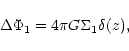
A model of the thin shell expanding into a uniform ambient medium
is developed.
Density perturbations are described using equations with linear
and quadratic terms, and the linear and the nonlinear solutions are
compared.
We follow the time evolution of the fragmentation process and separate
the well
defined fragments. Their mass spectrum is compared to observations and we
also estimate their formation time.
Key words: hydrodynamics - instabilities - stars: formation - ISM: bubbles - ISM: kinematics and dynamics - galaxies: ISM
The analysis of the stability of a pressure-confined slab performed by Elmegreen & Elmegreen (1978) has been extended to spherical expanding shocks by Vishniac (1983). The time development of the gravitational collapse of linear perturbations in decelerating, isothermal shocked layers has been examined numerically and analytically by Elmegreen (1989, 1994). The purely hydrodynamical nonlinear instability has been discussed by Vishniac (1994). In this paper, we continue with nonlinear analysis of the gravitational instability of spherically symmetric shells expanding into stationary homogeneous medium.
We modify the approach adopted by Fuchs (1996) who described the fragmentation of uniformly rotating self-gravitating disks. If some conditions are fulfilled, the expanding shell may become gravitationally unstable and break to fragments. The inclusion of higher order terms helps to determine with better accuracy than the linear analysis when, where and how quickly it happens.
The Rayleigh-Taylor (R-T) instability is not expected to develop in the situation explored because a spherical shock expanding into the homogeneous interstellar medium is always decelerated collecting stationary ambient medium. R-T instabilities may be important in different situations when the density of the ambient medium drops down sufficiently quickly so that the shell can accelerate mixing hot and cold gas components. This is the case of very active SF regions where the shell interacts with previously formed fragments. The region 30 Doradus in LMC may serve as an example of R-T instability in action as described by Redman et al. (1999).
For highly supersonic flows multiple shocks may develop (Falle 1981), but at that time the shells are gravitationally stable due to squeezing connected to the fast expansion. Later, when they decelerate to velocities less than 50 kms-1, the gravity starts to be important, while radiative instabilities of the outer shock described by Strickland & Blondin (1995) loose their influence.
This work may be extended to nonspherical oscillations using the formalism worked out by Bicák & Schmidt (1999) for cosmological applications. Here we also ignore the deviations from spherical symmetry resulting from initial asymmetry of the energy input. In a smooth medium with only large scale density gradients the shell approaches quickly the spherical symmetry as demonstrated by Bisnovatyi-Kogan & Blinnikov (1982). Nonradial perturbations resulting from inhomogeneities of the ambient medium and variations of the shell surface density will be discussed in a subsequent paper.
|
(1) |
 |
(2) |
 |
(3) |
 |
(8) |
 |
(9) |
In a subsequent paper, we shall also discuss
the instability in non-spherical shells: the values of ![]() and
and
![]() will be taken from numerical simulations.
will be taken from numerical simulations.
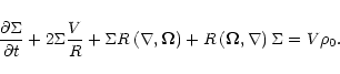
We consider the cold and thin shell of radius R surrounding the
hot interior
and expanding with velocity V into a uniform medium of density ![]() .
The intrinsic surface density of the shell
.
The intrinsic surface density of the shell ![]() is composed
of unperturbed part
is composed
of unperturbed part ![]() plus the perturbation
plus the perturbation ![]() (
(
![]() ).
Perturbation
).
Perturbation ![]() results from the flows on the surface of
the shell redistributing the accumulated mass.
We assume that
results from the flows on the surface of
the shell redistributing the accumulated mass.
We assume that ![]() corresponds to R as
corresponds to R as
![]() ,
which means that all the encountered mass is
accumulated to the shell.
(It comes from
,
which means that all the encountered mass is
accumulated to the shell.
(It comes from
![]() .)
.)
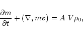
The mass conservation law in a small
area on the surface of the shell is
![\begin{figure}
\par\includegraphics[width=7.6cm]{grav_inst_shell.fig1.eps}\end{figure}](/articles/aa/full/2001/29/aah2488/img54.gif) |
Figure 1:
The coordinates on the shell
surface:
|
| Open with DEXTER | |
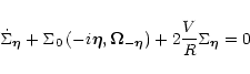
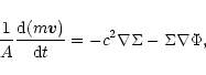
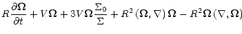
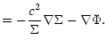
With
![]() we obtain continuity equation in a form
we obtain continuity equation in a form
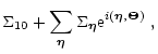
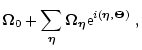
We assume a small perturbation of the shell surface density
![]() which evolves due to surface
flows given with velocity
which evolves due to surface
flows given with velocity ![]() .
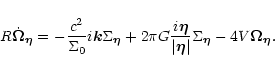
The perturbed hydrodynamical Eqs. (11), (13) and
the perturbed Poisson Eq. (14) have form
.
The perturbed hydrodynamical Eqs. (11), (13) and
the perturbed Poisson Eq. (14) have form
The perturbation of the surface density ![]() and the angular velocity
of the surface flows
and the angular velocity
of the surface flows
![]() can be written as
can be written as
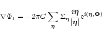
The solution of the Poisson Eq. (17)
 |
(20) |
 |
(22) |
 |
(23) |
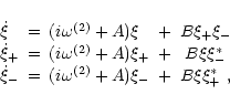
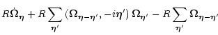
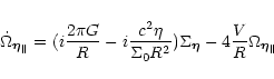
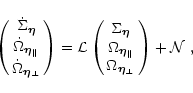
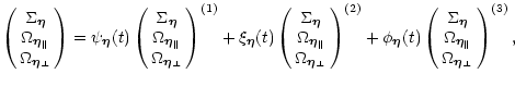
We get the set of equations
 |
(30) |
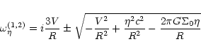
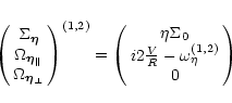
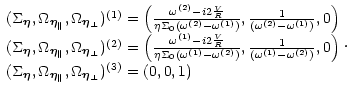
The related eigenvectors are
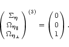 |
(32) |
| |
Figure 2:
The time dependence of the imaginary part of the
|
| Open with DEXTER | |
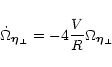
Since the eigenvalues
![]() depend on
depend on
![]() through the relation (29), the maximum
perturbation growth rate
through the relation (29), the maximum
perturbation growth rate
![]() can be found:
can be found:
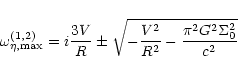 |
(33) |
 |
(34) |
 |
(35) |
 |
(37) |
 |
|||
 |
(40) |
Equation (44) is decoupled from the others and
its solution is the decrease of the
initial value of ![]() .
Equations (42) and (43) are coupled through the
linear and nonlinear terms. The interaction through
the linear terms is weak,
since the coupled linear terms have smaller amplitudes compared to
linear terms and they decrease with time due to their dependence on the time
derivatives of the eigenvectors, which are very small in the later stages of
the shell evolution. The coupling through the nonlinear terms leads to the
terms of the third and higher orders, which can be neglected with respect to
quadratic terms.
Furthermore, the solution of the Eq. (42) has
a decreasing character, because the first term on the right side, which
includes the "stable''
.
Equations (42) and (43) are coupled through the
linear and nonlinear terms. The interaction through
the linear terms is weak,
since the coupled linear terms have smaller amplitudes compared to
linear terms and they decrease with time due to their dependence on the time
derivatives of the eigenvectors, which are very small in the later stages of
the shell evolution. The coupling through the nonlinear terms leads to the
terms of the third and higher orders, which can be neglected with respect to
quadratic terms.
Furthermore, the solution of the Eq. (42) has
a decreasing character, because the first term on the right side, which
includes the "stable''
![]() ,
dominates.
Equation (43) is the most interesting one, because it has
,
dominates.
Equation (43) is the most interesting one, because it has
![]() in
the first linear term, and only the
in
the first linear term, and only the
![]() can be imaginary negative,
which has meaning of instability.
The explicit form of the Eq. (43) is
can be imaginary negative,
which has meaning of instability.
The explicit form of the Eq. (43) is
![\begin{figure}
\par\includegraphics[width=8.3cm]{grav_inst_shell.fig3.eps}\end{figure}](/articles/aa/full/2001/29/aah2488/img169.gif) |
Figure 3: The evolution of the maximum perturbation of the surface density in the case when the initial values of linear and nonlinear terms of perturbation are in phase. |
| Open with DEXTER | |
Demanding
![]() we obtain from geometrical consideration:
we obtain from geometrical consideration:
 |
(47) |
 |
(48) |
 |
(49) |
![\begin{figure}
\par\includegraphics[width=8cm]{grav_inst_shell.fig4.eps}\end{figure}](/articles/aa/full/2001/29/aah2488/img188.gif) |
Figure 4: The solution of the set of Eqs. (47) with the initial conditions corresponding to Fig. 3. |
| Open with DEXTER | |
The set of Eqs. (47) can be solved numerically.
We start at the time ![]() which is the time when the instability begins
(imaginary part of
which is the time when the instability begins
(imaginary part of
![]() starts to be negative).
First we select real and imaginary parts of all
initial perturbation amplitudes
starts to be negative).
First we select real and imaginary parts of all
initial perturbation amplitudes
![]() ,
which have the meaning of initial perturbations of the surface density
and of the velocity, such that they correspond to
,
which have the meaning of initial perturbations of the surface density
and of the velocity, such that they correspond to
![]() .
The magnitude of these perturbations in physical values
can be computed from the eigenvectors (31).
.
The magnitude of these perturbations in physical values
can be computed from the eigenvectors (31).
The solution is determined by parameters of two types: the first ones,
as speed of sound c in the shell, are constant values, the second ones, as
the radius of the shell R(t), the expansion velocity V(t)
and its time derivative
and the surface density
![]() and its time derivative, are functions
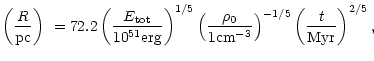
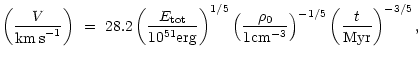
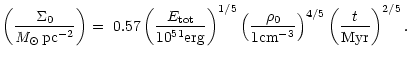
of time. We can get them either from the analytical Sedov
solution (4-6),
or from the numerical simulations of the expanding HI shells described by
Ehlerová et al. (1997). In this paper we use the Sedov solution
(Eqs. 4-6) with following
parameters: total energy
and its time derivative, are functions
of time. We can get them either from the analytical Sedov
solution (4-6),
or from the numerical simulations of the expanding HI shells described by
Ehlerová et al. (1997). In this paper we use the Sedov solution
(Eqs. 4-6) with following
parameters: total energy
![]() ,
density of ambient medium
,
density of ambient medium
![]() ,
average molecular weight
,
average molecular weight ![]() ,
sound speed in the
shell
,
sound speed in the
shell
![]() .
.
The time evolution of ![]() and
and ![]() are presented
in Figs. 3, 5, and 7 and the corresponding
amplitudes of
real and imaginary parts of
are presented
in Figs. 3, 5, and 7 and the corresponding
amplitudes of
real and imaginary parts of
![]() for the first two cases
in Figs. 4 and 6.
We can distinguish two situations: the linear and non-linear parts of the
perturbation are in phase, so that they support each other,
which is seen in Figs. 3 and 4,
or they are in anti-phase, so that the nonlinear
contribution slows down the linear growth of perturbation, as it is visible in
Figs. 5 and 6.
Contribution of the non-linear terms depends on the shape of the forming
fragments, i.e. on the value of the amplitude functions
for the first two cases
in Figs. 4 and 6.
We can distinguish two situations: the linear and non-linear parts of the
perturbation are in phase, so that they support each other,
which is seen in Figs. 3 and 4,
or they are in anti-phase, so that the nonlinear
contribution slows down the linear growth of perturbation, as it is visible in
Figs. 5 and 6.
Contribution of the non-linear terms depends on the shape of the forming
fragments, i.e. on the value of the amplitude functions
![]() .
Figures 3-6 show the extreme cases of that contribution.
Intermediate cases, keeping the initial value of the
perturbation in surface density at the
same level,
.
Figures 3-6 show the extreme cases of that contribution.
Intermediate cases, keeping the initial value of the
perturbation in surface density at the
same level,
![]() ,
are given in
Fig. 7.
We can also see in Fig. 3 that the maximum contribution
of nonlinear terms to
the value of the perturbed surface density, at the time when
,
are given in
Fig. 7.
We can also see in Fig. 3 that the maximum contribution
of nonlinear terms to
the value of the perturbed surface density, at the time when
![]() ,
is
,
is ![]() 25% of the linear value.
25% of the linear value.
![\begin{figure}
\par\includegraphics[width=8.4cm]{grav_inst_shell.fig5.eps}\end{figure}](/articles/aa/full/2001/29/aah2488/img194.gif) |
Figure 5: The evolution of the maximum perturbation of the surface density in the case when the initial values of linear and nonlinear terms of perturbation are in anti-phase. |
| Open with DEXTER | |
All the curves start at the instability time ![]() :
functions
:
functions
![]() ,
,
![]() and
and
![]() grow,
although the absolute value of the appropriate amplitude functions
grow,
although the absolute value of the appropriate amplitude functions
![]() ,
,
![]() and
and
![]() descend during the short time after the instability begins.
It is because
descend during the short time after the instability begins.
It is because
![]() ,
,
![]() and
and
![]() are
connected to the amplitude functions through the eigenvector (31),
whose
are
connected to the amplitude functions through the eigenvector (31),
whose ![]() part is always growing with time.
part is always growing with time.
The surface density ![]() at any point of the tangential plane
may be computed at any expansion time after
at any point of the tangential plane
may be computed at any expansion time after ![]() using
eigenvectors (31) and Eq. (18)
written for modes
using
eigenvectors (31) and Eq. (18)
written for modes
![]() .
In Fig. 8 we show the distribution of the
surface density
.
In Fig. 8 we show the distribution of the
surface density ![]() and in Fig. 9 the velocity field of
the surface flows
and in Fig. 9 the velocity field of
the surface flows ![]() in the tangential plane for
in the tangential plane for
![]() in the case when the
initial perturbations have
linear terms in phase with the nonlinear terms corresponding to
Figs. 3
and 4 at the time
in the case when the
initial perturbations have
linear terms in phase with the nonlinear terms corresponding to
Figs. 3
and 4 at the time
![]() .
Figures 10 and
11 give
.
Figures 10 and
11 give ![]() and
and ![]() in the tangential plane at the
same time for the case when the linear and nonlinear terms of the
initial perturbation are in anti-phase corresponding to Figs. 5 and
6. In the former case, the fragments are well defined and the
density peaks are separated one from another with
deep depressions in
in the tangential plane at the
same time for the case when the linear and nonlinear terms of the
initial perturbation are in anti-phase corresponding to Figs. 5 and
6. In the former case, the fragments are well defined and the
density peaks are separated one from another with
deep depressions in ![]() .
In the later case, there are high
surface density chains with no distinct peaks and we cannot separate
individual fragments.
.
In the later case, there are high
surface density chains with no distinct peaks and we cannot separate
individual fragments.
![\begin{figure}
\par\includegraphics[width=7.9cm]{grav_inst_shell.fig6.eps}\end{figure}](/articles/aa/full/2001/29/aah2488/img202.gif) |
Figure 6: The solution of the set of Eqs. (47) with the initial conditions corresponding to Fig. 5. |
| Open with DEXTER | |
![\begin{figure}
\par\includegraphics[width=8.4cm]{grav_inst_shell.fig7.eps}\end{figure}](/articles/aa/full/2001/29/aah2488/img203.gif) |
Figure 7: The evolution of the maximum perturbation of the surface density for intermediate phase-shifts between initial values of the linear and nonlinear terms of perturbation. |
| Open with DEXTER | |
We measure
the total mass concentrated in one of the well defined
fragments shown in Fig. 8. The mass of this fragment
is given
in Fig. 12 as a function of time.
It decreases because the decrease of its size, which is proportional to
![]() ,
and increases because the
accumulation of the ambient medium and surface flows. After
,
and increases because the
accumulation of the ambient medium and surface flows. After ![]() the
resulting mass of the fragment
decreases, since the influence of the size shrinking dominates.
This happens when the magnitude of
the
resulting mass of the fragment
decreases, since the influence of the size shrinking dominates.
This happens when the magnitude of
![]() is larger
then the amplitude of the surface flows
is larger
then the amplitude of the surface flows
![]() (see Fig. 13).
The magnitude of
(see Fig. 13).
The magnitude of
![]() decreases with time and
decreases with time and
![]() increases, and at
increases, and at
![]() they are equal. Since then the inflow dominates and the
fragment mass growths.
they are equal. Since then the inflow dominates and the
fragment mass growths.
| |
Figure 8:
The distribution of |
| Open with DEXTER | |
| |
Figure 9:
The velocity vectors of the surface flows |
| Open with DEXTER | |
After ![]() ,
when the first mode begins to be gravitationally unstable,
more and more modes are unstable and the interval of instability growths.
In Fig. 14 we give the values of the fragmentation integral
,
when the first mode begins to be gravitationally unstable,
more and more modes are unstable and the interval of instability growths.
In Fig. 14 we give the values of the fragmentation integral
![]() as defined in (36) as a function of time.
This shows at any time the level of development of a fragment with given
as defined in (36) as a function of time.
This shows at any time the level of development of a fragment with given
![]() .
.
| |
Figure 10: The same as in Fig. 8 at the same time for the perturbation shown in Figs. 5 and 6. |
| Open with DEXTER | |
| |
Figure 11:
The velocity vectors of the surface flows |
| Open with DEXTER | |
![\begin{figure}
\par\includegraphics[width=8.3cm]{grav_inst_shell.fig12.eps}\end{figure}](/articles/aa/full/2001/29/aah2488/img212.gif) |
Figure 12: The time evolution of total mass in a well defined fragment. |
| Open with DEXTER | |
![\begin{figure}
\par\includegraphics[width=8.3cm]{grav_inst_shell.fig13.eps}\end{figure}](/articles/aa/full/2001/29/aah2488/img214.gif) |
Figure 13:
|
| Open with DEXTER | |
![\begin{figure}
\par\includegraphics[width=8.2cm]{grav_inst_shell.fig14.eps}\end{figure}](/articles/aa/full/2001/29/aah2488/img215.gif) |
Figure 14:
The time evolution of the fragmentation integral
|
| Open with DEXTER | |
![\begin{figure}
\par\includegraphics[width=8.1cm]{grav_inst_shell.fig15.eps}\end{figure}](/articles/aa/full/2001/29/aah2488/img216.gif) |
Figure 15: The mass spectrum of fragments. The straight line is the power law fit of the decreasing part of the spectrum m-1.4. |
| Open with DEXTER | |
Mass
![]() of a fragment, which is related to
of a fragment, which is related to
![]() ,
may be defined as
,
may be defined as
 |
(51) |
![\begin{figure}
\par\includegraphics[width=8.3cm]{grav_inst_shell.fig16.eps}\end{figure}](/articles/aa/full/2001/29/aah2488/img231.gif) |
Figure 16:
Dependence of the fragmentation time on the initial
perturbation of the surface density. The vertical line gives the time when
the value of
|
| Open with DEXTER | |
The decreasing part of the mass spectrum can be approximated
as a power law
![]() :
the fit of the this part of
:
the fit of the this part of
![]() gives
gives
![]() ,
which is close to the observed
mass spectrum of GMC in the Milky Way: Combes(1991)
gives
,
which is close to the observed
mass spectrum of GMC in the Milky Way: Combes(1991)
gives
![]() .
NANTEN survey of the CO emission of the LMC (Fukui 2001) gives steeper
slope of
.
NANTEN survey of the CO emission of the LMC (Fukui 2001) gives steeper
slope of
![]() ,
which may be explained in the connection to higher level of random
velocities in the LMC compared to the Milky Way
resulting in the deficit of high mass clouds.
,
which may be explained in the connection to higher level of random
velocities in the LMC compared to the Milky Way
resulting in the deficit of high mass clouds.
The evolution of the maximum perturbation of the surface density
can be used to determine the fragmentation time ![]() of the shell.
Because at advanced stages the value of the maximum
perturbation rises steeply with the time (see e.g. Fig. 3), we
define
of the shell.
Because at advanced stages the value of the maximum
perturbation rises steeply with the time (see e.g. Fig. 3), we
define ![]() as the time, when maximum perturbation of the surface density is
equal to the unperturbed value:
as the time, when maximum perturbation of the surface density is
equal to the unperturbed value:
![]() .
Using the fragmentation integral
.
Using the fragmentation integral
![]() we may compare the
development level of different fragments at
we may compare the
development level of different fragments at ![]() (see Fig. 14).
We can say that the most frequent
fragments are also the most developed, the more massive form only later.
(see Fig. 14).
We can say that the most frequent
fragments are also the most developed, the more massive form only later.
![]() depends on the
initial conditions of the set of Eq. (47). They correspond
to the initial perturbation of the surface density. We can set them
to the value typical for the inhomogeneities in the clumpy interstellar
medium (
depends on the
initial conditions of the set of Eq. (47). They correspond
to the initial perturbation of the surface density. We can set them
to the value typical for the inhomogeneities in the clumpy interstellar
medium (
![]() ), which is at
), which is at ![]() :
:
![]() .
.
The dependence of ![]() on the value of the initial perturbation,
on the value of the initial perturbation,
![]() ,
is shown in
Fig. 16. Fragments form since
,
is shown in
Fig. 16. Fragments form since
![]() ,
for the largest
perturbations, to
,
for the largest
perturbations, to
![]() ,
for the smallest perturbations.
The spread in
,
for the smallest perturbations.
The spread in ![]() for given
for given
![]() is connected
to the different shape of the perturbation as shown in
Fig. 7. This time may be compared to the fragmentation
time
is connected
to the different shape of the perturbation as shown in
Fig. 7. This time may be compared to the fragmentation
time
![]() obtained for
obtained for
![]() from the linear analysis
defined as a time when
from the linear analysis
defined as a time when
![]() .
.
We evaluate the time evolution of perturbations on the surface of an
expanding shell. We complement the linear analysis of the gravitational
fragmentation process with the inclusion of
nonlinear terms, and we compute the time evolution of fragments
after the time when the shell starts to be unstable.
Some initial perturbations develop into well separated fragments and we
estimate the time evolution of the mass of a fragment, the mass
spectrum of fragments, and the spread in their formation time.
The computed mass spectrum is
close to the observed mass distribution
of GMC in the Milky Way, but slightly flatter than the mass spectrum of
molecular clouds observed in the LMC.
This may be related to higher level of random motions in the LMC compared
to the Milky Way, which
restricts the formation of late time massive
fragments and steepen the resulting mass spectrum.
Also interesting is that the more massive fragments
form at later times of the shell evolution than the less massive
fragments. The formation time
depends on the value of the initial perturbation:
![]() .
Large density fluctuations shorten this time and thus in the disturbed ISM
with large density fluctuations the fragments form sooner than in quiet
and smooth ISM where the density fluctuations are small.
.
Large density fluctuations shorten this time and thus in the disturbed ISM
with large density fluctuations the fragments form sooner than in quiet
and smooth ISM where the density fluctuations are small.
Acknowledgements
We would like to thank Burkhard Fuchs and to anonymous referee for valuable comments. This work was inspired by the paper on the fragmentation of uniformly rotating disks by Fuchs (1996). We are also grateful for an enlighting discussions with B. Fuchs in April 1998 and in March 2000 at Star 2000 conference in Heidelberg. The authors gratefully acknowledge financial support by the Grant Agency of the Academy of Sciences of the Czech Republic under the grant No. A 3003705/1997 and support by the grant project of the Academy of Sciences of the Czech Republic No. K1048102.
![\begin{displaymath}\omega_{\rm BGE} = -{3 V \over R} + \left[{V^2 \over R^2} + \left( \pi G \Sigma_0
\over c \right)^2\right]^{1/2},
\end{displaymath}](/articles/aa/full/2001/29/aah2488/img31.gif)


![$\displaystyle \left.
\left.
+\left( i2\frac{V}{R}-\omega^{(2)}\right) \xi_{\vec...
...]
\frac{(\vec\eta-\vec\eta' , \vec\eta')}{\vert\vec\eta-\vec\eta'\vert}
\right.$](/articles/aa/full/2001/29/aah2488/img151.gif)
![$\displaystyle \left.
\left.
\left.
\omega^{(2)}\right) \xi_{\vec\eta'} \right]
...
...vert\vec\eta\vert}
\right\}
- \frac{i}{\left( \omega^{(1)}-\omega^{(2)}\right)}$](/articles/aa/full/2001/29/aah2488/img158.gif)
![$\displaystyle \left.
\left.
\xi_{\vec\eta-\vec\eta'} \right]
\frac{(\vec\eta-\v...
...p}, \vec\eta)}{\vert\vec\eta-\vec\eta'_{\perp}\vert\vert\vec\eta\vert}
\right\}$](/articles/aa/full/2001/29/aah2488/img160.gif)
![$\displaystyle \left\{ \left[
\left( i2\frac{V}{R}-\omega^{(1)}\right) \psi_{\ve...
...c{V}{R}-\omega^{(2)}\right) \xi_{\vec\eta'} \right]
\vert\vec\eta'\vert
\right.$](/articles/aa/full/2001/29/aah2488/img161.gif)