A&A 374, 348-357 (2001)
DOI: 10.1051/0004-6361:20010622
L. Olmi![]()
LMT/GTM Project, Dept. of Astronomy, 815J Lederle GRT Tower B, University of Massachusetts, 710 N. Pleasant st., Amherst, MA 01003, USA
Received 6 March 2001 / Accepted 27 April 2001
Abstract
It is well known that the water vapor in the troposphere plays a
fundamental role in radio propagation. The refractivity of water vapor is
about 20 times greater in the radio range than in near-infrared or
optical regimes. As a consequence, phase fluctuations at frequencies
higher than about 1 GHz are predominantly caused by fluctuations in the
distribution of water vapor, and thus radio seeing at these frequencies
is predominantly caused by tropospheric turbulence.
Radio seeing shows up on filled-aperture telescopes as an anomalous
refraction (AR), i.e. an apparent displacement of a radio source from its
nominal position, corrected for large-scale refractive effects.
The magnitude of this effect, as a fraction of the beam width, is
bigger on larger telescopes and thus its impact on the pointing is likely
to become critically important in the next generation of electrically
large filled-aperture radio telescopes (
![]() )
and in
particular on the Large Millimeter Telescope. AR effects are expected
to reduce the total effective observing time at the highest frequencies and will
affect on-the-fly mapping. Here we present the results of systematic
AR measurements carried out with the 13.7-m telescope of the Five College
Radio Astronomy Observatory. The measured AR pointing errors range from
1''-3'' (winter) to about 20'' (summer) and most of the events last less
than about 4 s. We analysed the structure function, power spectrum and Allan
variance of the data and we have carried out a statistical analysis
to identify correlations of the statistical functions
with selected observing parameters such as precipitable water vapor,
time of day, season and elevation angle. Our results suggest that
uncompensated AR may be the most important dynamic environmental source
of pointing errors on the
new large radio telescopes (ALMA, GBT, LMT, SRT) and may guide
the design of active AR-compensation devices and help allocating
suitable observing time through dynamic scheduling.
)
and in
particular on the Large Millimeter Telescope. AR effects are expected
to reduce the total effective observing time at the highest frequencies and will
affect on-the-fly mapping. Here we present the results of systematic
AR measurements carried out with the 13.7-m telescope of the Five College
Radio Astronomy Observatory. The measured AR pointing errors range from
1''-3'' (winter) to about 20'' (summer) and most of the events last less
than about 4 s. We analysed the structure function, power spectrum and Allan
variance of the data and we have carried out a statistical analysis
to identify correlations of the statistical functions
with selected observing parameters such as precipitable water vapor,
time of day, season and elevation angle. Our results suggest that
uncompensated AR may be the most important dynamic environmental source
of pointing errors on the
new large radio telescopes (ALMA, GBT, LMT, SRT) and may guide
the design of active AR-compensation devices and help allocating
suitable observing time through dynamic scheduling.
Key words: atmospheric effects - methods: observational - telescopes
Radio-seeing effects on centimeter- and millimeter-wavelength interferometers are a consequence of the inhomogeneously distributed atmospheric water vapor which can cause spatial and temporal variations in the optical path length of radio waves. Several studies of the problem of phase fluctuations with both centimeter (e.g., Armstrong & Sramek 1982) and millimeter (e.g., Bieging et al. 1984; Olmi & Downes 1992; Wright 1996) interferometers have led to the development of a number of radiometric devices to compensate for these fluctuations and restore the uncorrupted phase off-line (e.g., Bremer 1995; Marvel & Woody 1998).
On the other hand, radio seeing on filled-aperture telescopes shows up as
an anomalous refraction (AR), i.e., an apparent displacement of a radio
source from its true position, caused by the phase difference introduced
between the opposite extremities of the receiving aperture because
the propagation paths traverse air masses of varying humidity.
AR pointing effects caused by turbulence in the "wet'' atmosphere
are similar to the "quivering'' of stars observed with visual-wavelength
telescopes, which are also known as angle of arrival fluctuations
in the field of clear- or dry-air propagation effects
(see, e.g., Fante 1975; Lawrence & Strohbehn 1970).
The magnitude of this effect, as a fraction of the beam width, is bigger
on larger telescopes and thus its impact on the pointing is likely
to become critically important in the next generation of electrically
large filled-aperture radio telescopes (
![]() ), and especially in
the case of the Large Millimeter Telescope (or "Gran Telescopio Milimetrico'',
in Spanish, LMT/GTM; see Olmi 1998; Kaercher & Baars 2000)
with a
), and especially in
the case of the Large Millimeter Telescope (or "Gran Telescopio Milimetrico'',
in Spanish, LMT/GTM; see Olmi 1998; Kaercher & Baars 2000)
with a
![]() at
at ![]() mm and a required pointing accuracy at
this wavelength <1''.
mm and a required pointing accuracy at
this wavelength <1''.
The first extensive measurements of AR were carried out by
Altenhoff et al. (1987), Downes & Altenhoff (1990), and also
Church & Hills (1990) who found that AR events are characterized by
angular displacements of the
sources from their true positions by a few arc seconds, in both azimuth and
elevation, for a few seconds of time, but occasionally showing much larger
events that could last for tens of seconds. This is similar to what is
observed in near-infrared astronomy, where, for small telescope
diameter to Fried parameter ratio,
![]() (the
Fried parameter represents the seeing cell size), the
short-exposure point spread function (PSF) randomly moves in the
focal plane (e.g., Close & McCarthy 1994).
On the new large radio telescopes that are either under construction
(GBT
(the
Fried parameter represents the seeing cell size), the
short-exposure point spread function (PSF) randomly moves in the
focal plane (e.g., Close & McCarthy 1994).
On the new large radio telescopes that are either under construction
(GBT![]() , LMT) or beeing designed
(ALMA, SRT
, LMT) or beeing designed
(ALMA, SRT![]() ), for which
), for which
![]() at the highest frequencies, phase gradients
across the antenna aperture (i.e., tilt) will dominate, but there will
be also higher order aberrations that can effectively broaden the primary beam
(Olmi 2000a).
In more recent years these projects have also
prompted serious investigations of techniques to compensate AR effects
(see Holdaway 1997; Butler 1997; Holdaway & Woody 1998;
Olmi 2000a, 2000b).
at the highest frequencies, phase gradients
across the antenna aperture (i.e., tilt) will dominate, but there will
be also higher order aberrations that can effectively broaden the primary beam
(Olmi 2000a).
In more recent years these projects have also
prompted serious investigations of techniques to compensate AR effects
(see Holdaway 1997; Butler 1997; Holdaway & Woody 1998;
Olmi 2000a, 2000b).
There were therefore several reasons to carry out an extensive, systematic study of the AR effects using a single-dish antenna: (i) AR is the most critical dynamic environmental source of pointing errors on large millimeter and submillimeter telescopes; (ii) the measurements of phase fluctuations with millimeter interferometers and "seeing monitors'' is sensitive to the relative orientation of the baseline and the wind direction (Lay 1997), and they are often carried out over large spatial scales compared to the diameter of single-dish antennas; (iii) it is important to determine the potential effects of AR during On-The-Fly (OTF) mapping; (iv) the next generation of mm-wave telescopes represent big time, effort, and money investments and thus must meet their design goals and yield a high observing efficiency; (v) a better knowledge of AR would also improve the design of active AR-compensation devices and help allocating suitable observing time through dynamic scheduling.
The main goal of this work is to
present the results of systematic AR observations carried
out with the 13.7-m telescope of the Five College Radio Astronomy
Observatory![]() (FCRAO) located in New Salem (USA) at an
elevation of 314 m above sea level.
They show that AR is clearly detectable with the FCRAO 60''
beam-width at 86 GHz even when the precipitable water vapor (PWV) is a
few mm only. Measured values range from as "little'' as 1''-2'' (winter) to as
much as 20'' (summer). The main purposes of these observations were:
(i) detect AR effects and characterize their magnitude (and time-scales)
as a function of time of the day, season, and elevation;
(ii) detect and measure systematic changes in AR statistical
properties (slopes, turn-overs, etc.).
Some results from an incomplete data sample can be found in
Olmi (2000b, 2001) where we also discuss
the basic technical problems of a tip-tilt compensation device at millimeter
wavelengths for the LMT as well as other related issues.
The outline of the paper is as follows: in Sect. 2
we describe the measurement technique; in Sect. 3 we analyze and
discuss the AR data using several statistical functions;
finally, we draw our conclusions in Sect. 4.
(FCRAO) located in New Salem (USA) at an
elevation of 314 m above sea level.
They show that AR is clearly detectable with the FCRAO 60''
beam-width at 86 GHz even when the precipitable water vapor (PWV) is a
few mm only. Measured values range from as "little'' as 1''-2'' (winter) to as
much as 20'' (summer). The main purposes of these observations were:
(i) detect AR effects and characterize their magnitude (and time-scales)
as a function of time of the day, season, and elevation;
(ii) detect and measure systematic changes in AR statistical
properties (slopes, turn-overs, etc.).
Some results from an incomplete data sample can be found in
Olmi (2000b, 2001) where we also discuss
the basic technical problems of a tip-tilt compensation device at millimeter
wavelengths for the LMT as well as other related issues.
The outline of the paper is as follows: in Sect. 2
we describe the measurement technique; in Sect. 3 we analyze and
discuss the AR data using several statistical functions;
finally, we draw our conclusions in Sect. 4.
The AR observations have been carried out using the FCRAO
radome-enclosed 13.7-m telescope located in western Massachusetts.
The telescope site is characterized by flat terrain surrounded by
woods, with PWV values (calculated using the measured ground-level
dew point temperature) ranging from <1 mm in winter to more than
10 mm in summer time. The occurrence of AR was recorded by
tracking a strong SiO maser (![]() GHz) pointlike
source at the azimuth half-power points of the response pattern.
The source intensity was then compared with the
ON-source intensity to determine the apparent angular shift, assuming
a given main beam pattern that is well represented by a Gaussian profile
(Ladd & Heyer 1996). There is a tendency for the beam to be broader
at lower elevations, because of (mainly)
gravitational effects, but at 86 GHz the
maximum FWHM variation is about
GHz) pointlike
source at the azimuth half-power points of the response pattern.
The source intensity was then compared with the
ON-source intensity to determine the apparent angular shift, assuming
a given main beam pattern that is well represented by a Gaussian profile
(Ladd & Heyer 1996). There is a tendency for the beam to be broader
at lower elevations, because of (mainly)
gravitational effects, but at 86 GHz the
maximum FWHM variation is about ![]() % for elevations
% for elevations
![]()
![]() and is
and is ![]() 8% for elevations between
8% for elevations between
![]() and
and
![]() (Ladd & Heyer 1996). Because the pointing errors are obtained
through a relative measurement they are not affected by gain variations
as a function of elevation angle.
(Ladd & Heyer 1996). Because the pointing errors are obtained
through a relative measurement they are not affected by gain variations
as a function of elevation angle.
The pointing and focus of the telescope were checked at the
beginning of a new observing session and about every 30 min thereafter. The
typical absolute pointing accuracy was about 6'', although the critical
parameter of interest to AR measurements is the tracking accuracy (see below).
Likewise the ON-source intensity was checked before and after an
AR time series. Using this technique one measures the modified
angular distance, ![]() ,
of the target source from the beam center, i.e.
,
of the target source from the beam center, i.e.
![]() ,
where
,
where
![]() is the beam FWHM
(see Fig. 1 of Olmi 2000b).
is the beam FWHM
(see Fig. 1 of Olmi 2000b).
![]() is the quantity of
interest to determine the antenna pointing error, and
the data used in this work are time series of the observable
is the quantity of
interest to determine the antenna pointing error, and
the data used in this work are time series of the observable
![]() .
Further information about the
observing technique can be found in Olmi (2000b).
.
Further information about the
observing technique can be found in Olmi (2000b).
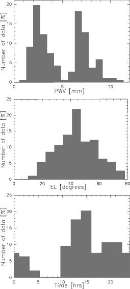 |
Figure 1: Histograms showing the distribution of the data as a function of PWV (top), elevation angle (middle) and local time (bottom), for combined data sample I and II. |
| Open with DEXTER | |
Two sets of data were obtained: a large
sample where the source intensity was sampled every
![]() s,
for as long as 5.5 min, and a smaller set of data with
s,
for as long as 5.5 min, and a smaller set of data with
![]() s
and with durations of up to 10 min.
The data sampled with = 3 s were obtained under cloud-free conditions
in the period of February 1999 to June 2000 and we will refer to them as
sample I. The data with = 1 s were obtained during similar and, very often,
during the same weather conditions as sample I during spring 2000, and
we will refer to them as sample II. The values of the outside temperature and
PWV were recorded during the observations. However, no data on wind speed and
direction were available.
The data are not uniformly distributed in the observing parameters' space.
In particular,
most of the data have been taken during conditions of either low or high PWV,
as shown in Fig. 1, due to the availabilty of observing time
during the regular observing season (when typically
s
and with durations of up to 10 min.
The data sampled with = 3 s were obtained under cloud-free conditions
in the period of February 1999 to June 2000 and we will refer to them as
sample I. The data with = 1 s were obtained during similar and, very often,
during the same weather conditions as sample I during spring 2000, and
we will refer to them as sample II. The values of the outside temperature and
PWV were recorded during the observations. However, no data on wind speed and
direction were available.
The data are not uniformly distributed in the observing parameters' space.
In particular,
most of the data have been taken during conditions of either low or high PWV,
as shown in Fig. 1, due to the availabilty of observing time
during the regular observing season (when typically
![]() mm) and during
the month of June before the receivers are shut down.
mm) and during
the month of June before the receivers are shut down.
 |
Figure 2:
Histograms of AR-induced angular displacements (
|
| Open with DEXTER | |
The range of spatial frequencies analyzed was ![]() 0.003 Hz to
a Nyquist frequency of
0.003 Hz to
a Nyquist frequency of
![]() Hz for sample I
and
Hz for sample I
and ![]() 0.002 Hz to
0.002 Hz to
![]() Hz for sample II.
Consequently, we were unable to observe AR events with time scales shorter
than
Hz for sample II.
Consequently, we were unable to observe AR events with time scales shorter
than
![]() s.
Our measurements carried out during very dry conditions in winter
(PWV<1 mm) indicate that the telescope tracking error
is <1'', which we then consider as the sensitivity limit of our
AR observations. No correlation was found between the AR pointing
error and various recorded telescope parameters, such as subreflector's
motors readings and the electronic levels of the AZ track.
s.
Our measurements carried out during very dry conditions in winter
(PWV<1 mm) indicate that the telescope tracking error
is <1'', which we then consider as the sensitivity limit of our
AR observations. No correlation was found between the AR pointing
error and various recorded telescope parameters, such as subreflector's
motors readings and the electronic levels of the AZ track.
Figure 2 shows the distribution of angular displacements observed on three days with different PWV of sample II. The data were taken during a short period of time (between 13:00 and 16:00 local time) in stable weather and thus during conditions of very similar PWV and temperature. Because the three histograms in Fig. 2 are not the average of many days of data, with very different conditions, they represent a good approximation of the AR probability density function (PDF) for a given PWV. Moreover, the air-mass range was approximately the same for each of the three days considered (1.1 to 1.6) and therefore the different widths of the histograms cannot be explained as an elevation effect (see Sect. 3.5 for a discussion about elevation effects).
 |
Figure 3:
Histograms of the duration of AR events for the same days shown in
Fig. 2 (line styles are the same). The bins have a width
|
| Open with DEXTER | |
The widths of the PDFs in Fig. 2 corresponding to about 75%
of the total area underneath the histograms are ![]() 6'' and
6'' and
![]() 4'' for the 26-MAY-2000 and the April 2000 data, respectively.
Therefore, during typical dry weather (PWV<4 mm, or
4'' for the 26-MAY-2000 and the April 2000 data, respectively.
Therefore, during typical dry weather (PWV<4 mm, or
![]() at the
FCRAO site) the magnitude of AR
can be of up to several arcseconds, although we cannot exclude that it
might be even larger on time-scales shorter than
at the
FCRAO site) the magnitude of AR
can be of up to several arcseconds, although we cannot exclude that it
might be even larger on time-scales shorter than
![]() .
In summer time at FCRAO, or during conditions of high PWV, the
AR pointing error can be a considerable fraction of the FCRAO beam-width.
All other observing conditions being approximately the same, the PWVseems to be a good tracer of AR activity (but see the important
discussion in Sect. 3.5) and may thus allow
an extrapolation of these results to other sites. We note, however, that
we obtained these values on a flat terrain and there is certainly more
turbulence on a mountain top. Therefore, under similar PWV conditions
we might expect more variations
in the AR-induced pointing errors measured on the LMT/GTM site, due to its
more complex topography, than on a large open site such as the FCRAO.
Furthermore, because the largest AR-induced pointing errors will occur at the
shortest wavelengths, and because it is likely that the LMT/GTM will operate
in this high-frequency regime only during conditions of low (
.
In summer time at FCRAO, or during conditions of high PWV, the
AR pointing error can be a considerable fraction of the FCRAO beam-width.
All other observing conditions being approximately the same, the PWVseems to be a good tracer of AR activity (but see the important
discussion in Sect. 3.5) and may thus allow
an extrapolation of these results to other sites. We note, however, that
we obtained these values on a flat terrain and there is certainly more
turbulence on a mountain top. Therefore, under similar PWV conditions
we might expect more variations
in the AR-induced pointing errors measured on the LMT/GTM site, due to its
more complex topography, than on a large open site such as the FCRAO.
Furthermore, because the largest AR-induced pointing errors will occur at the
shortest wavelengths, and because it is likely that the LMT/GTM will operate
in this high-frequency regime only during conditions of low (
![]() 5-10 m/s)
wind-speed, we should not expect that the reduced time-scale of AR events
resulting during conditions of high wind-speed will contribute to
average the AR effects down. It is clear, however, that extrapolating
these results to sites with different characteristics and at higher
frequencies is difficult as well as uncertain
and specific on-site measurements should be obtained.
5-10 m/s)
wind-speed, we should not expect that the reduced time-scale of AR events
resulting during conditions of high wind-speed will contribute to
average the AR effects down. It is clear, however, that extrapolating
these results to sites with different characteristics and at higher
frequencies is difficult as well as uncertain
and specific on-site measurements should be obtained.
We define the duration of an "AR event''
as the time interval between two measurements, preceeding and following a
peak (either positive or negative) in the AR time series, and having a
value of
![]() smaller than 50% of the peak value.
In Fig. 3 we show the distribution of the durations of the
apparent displacements of the source as observed on the same days as in
Fig. 2. Two interesting features can be seen: first, the three
histograms are remarkably similar and do not show any specific feature
associated with different PWVs.
Second, most (
smaller than 50% of the peak value.
In Fig. 3 we show the distribution of the durations of the
apparent displacements of the source as observed on the same days as in
Fig. 2. Two interesting features can be seen: first, the three
histograms are remarkably similar and do not show any specific feature
associated with different PWVs.
Second, most (
![]() 75%) of the events last less
than about 3-4 s. To first order, the typical duration of an AR event
is consistent with the time it takes a moist element to cross the dish and
it is expected to be longer on larger antennas (see Holdaway 1997).
Moreover, the distribution of the event durations has a tail which may
stretch to times
75%) of the events last less
than about 3-4 s. To first order, the typical duration of an AR event
is consistent with the time it takes a moist element to cross the dish and
it is expected to be longer on larger antennas (see Holdaway 1997).
Moreover, the distribution of the event durations has a tail which may
stretch to times ![]() 10-20 s, although these events are much rarer.
The AR events durations obtained using data from sample I have similar
distributions but they fail to show that most of the events are of very short
duration (see Olmi 2000b).
Therefore, observations that are short compared to the typical duration
of the AR events, as is the case in OTF mapping, will be seriously affected
by the AR pointing errors. Multiple sweeps across the source may somewhat
reduce the average pointing error but will incur in a flux density loss
and primary beam broadening anyway.
10-20 s, although these events are much rarer.
The AR events durations obtained using data from sample I have similar
distributions but they fail to show that most of the events are of very short
duration (see Olmi 2000b).
Therefore, observations that are short compared to the typical duration
of the AR events, as is the case in OTF mapping, will be seriously affected
by the AR pointing errors. Multiple sweeps across the source may somewhat
reduce the average pointing error but will incur in a flux density loss
and primary beam broadening anyway.
Are the longest AR events also the ones with larger magnitudes? To answer this question we generated the three-dimensional plots shown in Fig. 4 where the distribution of the data points is plotted as a function of the AR-induced pointing error and the corresponding event duration. The double-peak structure is due to the equal probability of having, for each duration time, either a positive (the angular distance of the target source from the center of the beam increases as an effect of AR) or negative (the target source approaches the beam center) pointing error. Clearly, the PDFs of the AR pointing errors are very similar at any given event duration, except of course for the total number of occurrences that decreases for longer durations as already discussed above. Therefore, our data show that while AR events of short duration are more likely to occur, the distribution of their magnitudes remains approximately constant. Multiple events that would show up as long duration ones are possible but they would be indistinguishable from individual events and we have not attempted any sophisticated procedure to select them.
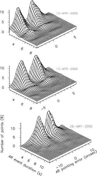 |
Figure 4: Distribution of the data points as a function of the event duration and pointing error, for the same days as in Fig. 2. |
| Open with DEXTER | |
The temporal structure function,
![]() where
where ![]() is the time lag, for the observable AR-induced pointing
error
is the time lag, for the observable AR-induced pointing
error
![]() can be defined as (Olmi 2000b):
can be defined as (Olmi 2000b):
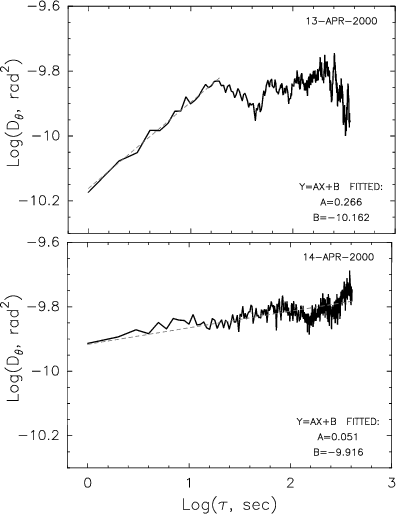 |
Figure 5: Top: example of structure function with a break in the slope and saturation at longer lag times. Bottom: example of structure function with no saturation. |
| Open with DEXTER | |
The distribution of ![]() and of
the intercept,
and of
the intercept,
![]() ,
are shown in Fig. 6 for the
entire set of data, i.e. samples I and II. Most of the slopes of
,
are shown in Fig. 6 for the
entire set of data, i.e. samples I and II. Most of the slopes of
![]() are
are
![]() 0.4 and the weighted average is
0.4 and the weighted average is
![]() .
However,
.
However,
![]() can vary over two orders of magnitude from about -4 to
about -2.
can vary over two orders of magnitude from about -4 to
about -2.
The AR structure function and the phase structure function measured
with interformeters are different, and this may also explain why in
many cases the AR structure function can saturate as shown
in Fig. 5.
The spatial phase structure function at a given time t is
defined as:
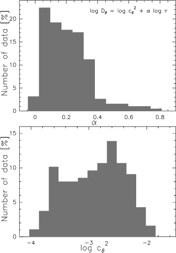 |
Figure 6:
Histograms showing the distribution of |
| Open with DEXTER | |
where ![]() is the wavefront phase measured at two positions separated
by the distance
is the wavefront phase measured at two positions separated
by the distance
![]() .
If we replace the baseline
.
If we replace the baseline
![]() with the distance
separating two points on the antenna diameter
with the distance
separating two points on the antenna diameter
![]() and assume that the
wavefront across the antenna is tilted with respect to the optical axis but
has no higher-order aberrations otherwise, then the phase difference,
and assume that the
wavefront across the antenna is tilted with respect to the optical axis but
has no higher-order aberrations otherwise, then the phase difference,
![]() ,
across the antenna aperture can be approximated as:
,
across the antenna aperture can be approximated as:
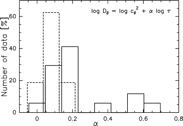 |
Figure 7:
Histogram showing the distribution of |
| Open with DEXTER | |
A comparison between Eq. (9) and
Fig. 6 shows that the measured value of
![]() is much smaller than the Kolmogorov value
is much smaller than the Kolmogorov value
![]() .
However, the
distribution in Fig. 6 could be explained if most of the data
were taken near or at saturation, i.e.
.
However, the
distribution in Fig. 6 could be explained if most of the data
were taken near or at saturation, i.e.
![]() ,
or if Taylor's
hypothesis is not entirely correct. If we use a typical
value of
,
or if Taylor's
hypothesis is not entirely correct. If we use a typical
value of
![]() m/s for the wind speed parallel to the ground
and a zenith angle of
m/s for the wind speed parallel to the ground
and a zenith angle of
![]() ,
and if we also assume that the
wind speed vector and the line of sight lie on the same plane, then:
,
and if we also assume that the
wind speed vector and the line of sight lie on the same plane, then:
In Fig. 7 we plot the histograms
of ![]() for the data with
for the data with
![]() and for those with
and for those with
![]() ,
and one can see that the distribution of the data taken at
lower elevations is skewed towards higher
,
and one can see that the distribution of the data taken at
lower elevations is skewed towards higher ![]() vales, as confirmed by their
weighted averages of 0.23 and 0.08 for the two histograms, respectively. The
data taken at higher elevations have no values of
vales, as confirmed by their
weighted averages of 0.23 and 0.08 for the two histograms, respectively. The
data taken at higher elevations have no values of
![]() .
.
Although Fig. 7 suggests that saturation (i.e., a smaller
slope of the structure function) is more likely
to be observed at higher elevation angles, we could not find any clear
correlation between
![]() and
and ![]() ,
as suggested by Eq. (11).
This may be due to: (i) wind speed vector not coplanar, on average,
with the telescope
line of sight, and (ii) distribution of elevation angles biased towards
intermediate values (see Fig. 1).
,
as suggested by Eq. (11).
This may be due to: (i) wind speed vector not coplanar, on average,
with the telescope
line of sight, and (ii) distribution of elevation angles biased towards
intermediate values (see Fig. 1).
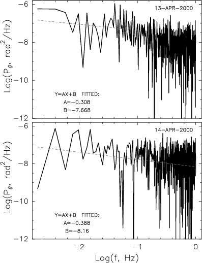 |
Figure 8: Power spectra of the same time series whose structure functions are shown in Fig. 5. In the top-panel a break in the slope of the spectrum can be seen at a frequency of about 0.05 Hz. |
| Open with DEXTER | |
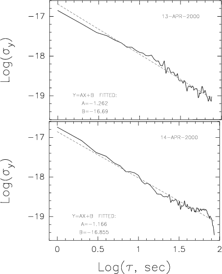 |
Figure 9: Allan standard deviations of the same time series whose structure functions are shown in Fig. 5. |
| Open with DEXTER | |
The one-sided power spectrum can also be calculated from the
![]() time series, and it is defined as:
time series, and it is defined as:
It can be shown that if the interferometer phase structure function
![]() then the one-dimensional temporal
phase power spectrum
then the one-dimensional temporal
phase power spectrum
![]() (Armstrong &
Sramek 1982).
Because the slope of the phase structure function,
(Armstrong &
Sramek 1982).
Because the slope of the phase structure function,
![]() ,
is the same as the slope of the AR structure function,
,
is the same as the slope of the AR structure function,
![]() ,
as shown by Eq. (9), one should
expect that if
,
as shown by Eq. (9), one should
expect that if
![]() then
then
![]() (see Sect. 3.5 for
a discussion of this point). The weighted average of the slopes of the
AR power spectra is -0.73, and we can compare this value with the
model of the angle of arrival spectrum obtained by Fante (1975).
If we use Fante's Eq. (84) with v=5 m/s we find that in the
frequency range
0.004-0.16 Hz the slope is
(see Sect. 3.5 for
a discussion of this point). The weighted average of the slopes of the
AR power spectra is -0.73, and we can compare this value with the
model of the angle of arrival spectrum obtained by Fante (1975).
If we use Fante's Eq. (84) with v=5 m/s we find that in the
frequency range
0.004-0.16 Hz the slope is ![]() -0.8, consistent
with the AR average value.
The intensity values of the power spectra (e.g., for the examples shown in
Fig. 8) are also consistent with Fante's model assuming the
turbulence outer scale is
-0.8, consistent
with the AR average value.
The intensity values of the power spectra (e.g., for the examples shown in
Fig. 8) are also consistent with Fante's model assuming the
turbulence outer scale is
![]() m and
m and
![]() m-1/3(see Sect. 3.5 for a discussion on the parameter
m-1/3(see Sect. 3.5 for a discussion on the parameter
![]() ).
).
The Allan variance is another useful method to describe the atmopsheric
phase fluctuations (see, e.g., Armstrong & Sramek 1982; Thompson et al. 1986; Olmi & Downes 1992; Wright 1996). The
Allan variance of the AR fluctuations removes linear drifts from
the data and is defined as:
We have carried out a statistical analysis of the data to
identify possible correlations of either the power law indices or
![]() with selected observing parameters such as PWV,
time of day, season and elevation angle.
with selected observing parameters such as PWV,
time of day, season and elevation angle.
Because as we mentioned earlier in Sect. 3.1 the PWVis one of the major environmental factors associated with the magnitude of the
AR errors, we first present in Fig. 10 the correlation
of
![]() with PWV. From the fit to our data we find the
empirical formula:
with PWV. From the fit to our data we find the
empirical formula:
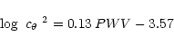 |
(14) |
We have previously seen in Eq. (10) that the structure coefficient
of AR is proportional to the phase structure coefficient, which can be written
for Kolmogorov turbulence (
![]() )
as (see, e.g., Roggemann
& Welsh 1996):
)
as (see, e.g., Roggemann
& Welsh 1996):
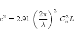 |
(15) |
 |
Figure 10:
Plot of
|
| Open with DEXTER | |
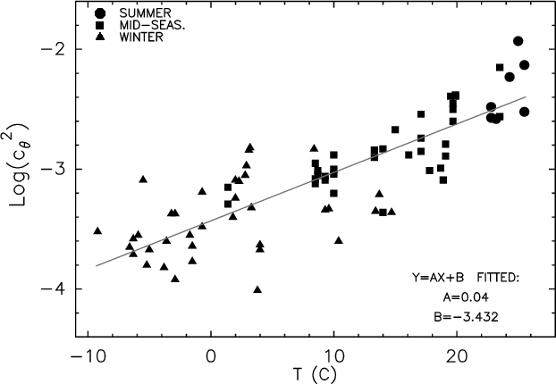 |
Figure 11:
Plot of
|
| Open with DEXTER | |
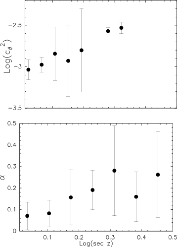 |
Figure 12:
Plots of
|
| Open with DEXTER | |
In Fig. 12 we show
![]() and
and ![]() plotted as a
function of
plotted as a
function of
![]() .
Because
.
Because
![]() shows a correlation with
the local time (see Fig. 13) we selected only data in the
13:00 to 16:00 time interval in the top panel of Fig. 12. However,
because
shows a correlation with
the local time (see Fig. 13) we selected only data in the
13:00 to 16:00 time interval in the top panel of Fig. 12. However,
because ![]() does not seem to correlate with time (see discussion below)
we used all data in the bottom panel of Fig. 12.
Despite some big error bars
it is clear from Fig. 12
that the AR structure coefficient tends to increase at larger zenith angles.
This trend was expected since for non-zenith angles Eq. (1)
must be rewritten as:
does not seem to correlate with time (see discussion below)
we used all data in the bottom panel of Fig. 12.
Despite some big error bars
it is clear from Fig. 12
that the AR structure coefficient tends to increase at larger zenith angles.
This trend was expected since for non-zenith angles Eq. (1)
must be rewritten as:
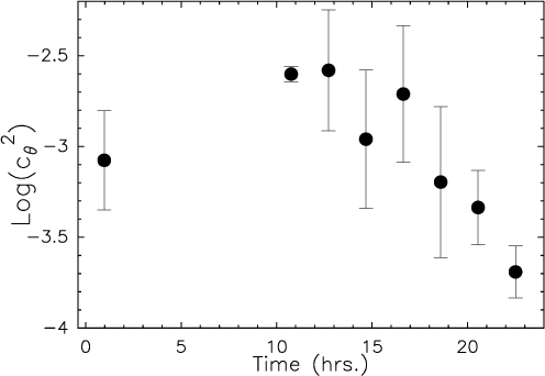 |
Figure 13:
Plot of
|
| Open with DEXTER | |
We then wanted to find out whether a correlation exists between
![]() and the local time. We present our results in
Fig. 13 where it can be clearly seen that the AR structure
coefficient tends to decrease during the afternoon and evening hours. The
night hours are less well sampled, and in particular we have no data between
approximately 05:00 and 09:00, as shown in Fig. 1; however,
the data suggest that a
and the local time. We present our results in
Fig. 13 where it can be clearly seen that the AR structure
coefficient tends to decrease during the afternoon and evening hours. The
night hours are less well sampled, and in particular we have no data between
approximately 05:00 and 09:00, as shown in Fig. 1; however,
the data suggest that a
![]() peak may be reached sometime before
10:00.
The day-night cycle of
peak may be reached sometime before
10:00.
The day-night cycle of
![]() follows a similar pattern
of both PWV and ambient temperature, and thus it seems to suggest that
this diurnal variation is associated with increased turbulence near the ground
during the day-time, as we suggested earlier in this section.
A variability of the structure coefficient with time was also found by
Olmi & Downes (1992) in the case of the phase structure function
measured with the IRAM interferometer. On the other hand, we find
no clear correlation between
follows a similar pattern
of both PWV and ambient temperature, and thus it seems to suggest that
this diurnal variation is associated with increased turbulence near the ground
during the day-time, as we suggested earlier in this section.
A variability of the structure coefficient with time was also found by
Olmi & Downes (1992) in the case of the phase structure function
measured with the IRAM interferometer. On the other hand, we find
no clear correlation between ![]() and the local time
whereas such a correlation was also observed by Olmi
& Downes.
and the local time
whereas such a correlation was also observed by Olmi
& Downes.
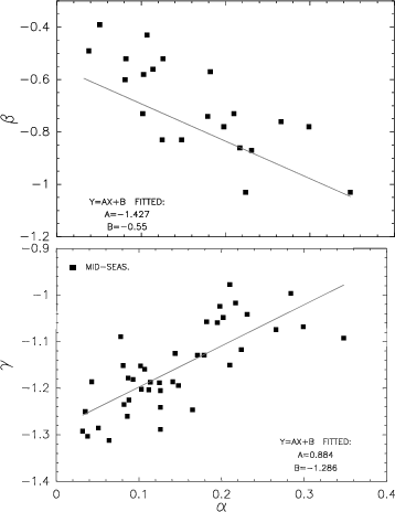 |
Figure 14:
Plots of |
| Open with DEXTER | |
In Fig. 14 we plot the indices of the power laws describing
the power spectrum and the Allan variance, defined in Eqs. (12)
and (13), as a function of the power law index describing the
structure function (sample II only). Clearly, ![]() and
and ![]() correlate with
correlate with ![]() ,
and the two best-fit lines are given by the
equations
,
and the two best-fit lines are given by the
equations
![]() and
and
![]() ,
which
are consistent with the predicted values of
,
which
are consistent with the predicted values of
![]() and
and
![]() ,
respectively, as described in Sect. 3.4.
This consistency between the measured best-fit values and the theoretical
values of the various power law slopes, obtained applying the standard model
of turbulence to the phase fluctuations of an interferometer, suggests
that the same model can also be applied to the AR fluctuations measured with
a single-dish antenna. In fact, in Sect. 3.3.2 we showed how the
structure functions of the phase and AR fluctuations can be related.
,
respectively, as described in Sect. 3.4.
This consistency between the measured best-fit values and the theoretical
values of the various power law slopes, obtained applying the standard model
of turbulence to the phase fluctuations of an interferometer, suggests
that the same model can also be applied to the AR fluctuations measured with
a single-dish antenna. In fact, in Sect. 3.3.2 we showed how the
structure functions of the phase and AR fluctuations can be related.
We have carried out systematic measurements of AR-induced pointing errors
with the radome-enclosed FCRAO 13.7 m telescope located in western
Masschusetts on a flat terrain, during the period February 1999
to June 2000. The data are based on the time series of the fluctuations of the
angular distance of the source from the beam center, as measured at the
-3 dB points. We have detected AR-induced pointing errors with the
FCRAO 60'' beam.
The measured values range from ![]() 2'' (winter) to
2'' (winter) to ![]() 20''(summer). The probability density distributions of the AR pointing errors
are narrower for low PWV and wider for high PWV, and during typical dry
weather (PWV<4 mm) the FWHM of the distributions can be of several
arcseconds.
We have also measured the duration of the individual "AR events'' and
found that most of them last less than 3-4 s, with tails
in the distribution stretching to
20''(summer). The probability density distributions of the AR pointing errors
are narrower for low PWV and wider for high PWV, and during typical dry
weather (PWV<4 mm) the FWHM of the distributions can be of several
arcseconds.
We have also measured the duration of the individual "AR events'' and
found that most of them last less than 3-4 s, with tails
in the distribution stretching to ![]() 10-20 s. Such short-duration
fluctuations will not be averaged out during a typical OTF scan and can
thus affect the reliability of OTF mapping on AR-limited telescopes.
10-20 s. Such short-duration
fluctuations will not be averaged out during a typical OTF scan and can
thus affect the reliability of OTF mapping on AR-limited telescopes.
Several statistical functions have been used to analyse the data. We
found that many structure functions can be fit with a single power law
of type
![]() ,
where
usually
,
where
usually
![]() and
and
![]() to -2.
The slope of the AR structure functions is much lower than that
of the phase structure functions measured with millimeter-wave
interferometers.
Power spectra and Allan variance plots can also be fit with single power laws,
and we found that the three different power law slopes correlate and are
consistent with the standard model of atmospheric turbulence.
The magnitude of the AR fluctuations, represented by the structure
coefficient,
to -2.
The slope of the AR structure functions is much lower than that
of the phase structure functions measured with millimeter-wave
interferometers.
Power spectra and Allan variance plots can also be fit with single power laws,
and we found that the three different power law slopes correlate and are
consistent with the standard model of atmospheric turbulence.
The magnitude of the AR fluctuations, represented by the structure
coefficient,
![]() ,
correlates well with PWV and ground-level
temperature, decreases with increasing elevation angle and also varies
during the day. These characteristics indicate that stronger AR
fluctuations are associated with increased convective activity
near the ground, which is typical of warmer, and more humid, weather
when strong thermal gradients create considerable ground-level turbulence.
Correlations of
,
correlates well with PWV and ground-level
temperature, decreases with increasing elevation angle and also varies
during the day. These characteristics indicate that stronger AR
fluctuations are associated with increased convective activity
near the ground, which is typical of warmer, and more humid, weather
when strong thermal gradients create considerable ground-level turbulence.
Correlations of ![]() with the observing parameters are still unclear.
with the observing parameters are still unclear.
Extrapolation of these results to other telescope sites, such as the LMT/GTM site, is uncertain because of the different latitude, elevation and terrain characteristics. However, it seems reasonable to expect similar AR effects during conditions of similar PWV and ambient temperature. If this is indeed the case then the expected magnitude of the AR-induced pointing errors can be comparable with the beam width of the LMT/GTM, under certain conditions, and all antenna measurements (OTF mapping, pointing, focusing, beam switching, etc.) would then be seriously affected. The LMT/GTM is currently studying the design of a radiometric wave front sensor to compensate AR effects.
Acknowledgements
This work was sponsored by the Advance Research Project Agency, Sensor Technology Office DARPA Order No. C134 Program Code No. 63226E issued by DARPA/CMO under contract No. MDA972-95-C-0004, and by the NSF grant AST-9725951. The author thanks M. Brewer and M. Heyer of FCRAO for help with the observing technique and reduction of some of the data used in this work.
![\begin{displaymath}{\cal D}_{\theta}(\tau) \equiv \,\,
\left <[\Delta\theta(t+\...
...a(t)]^2\right >\,
\, = \mbox{ $c_{\theta}$ }^2\, \tau^{\alpha}
\end{displaymath}](/articles/aa/full/2001/28/aah2735/img45.gif)
![\begin{displaymath}{\cal S}_{\phi}(\mbox{$b$ }) \equiv \,\,
\left <[\phi(\mbox{$r$ }+\mbox{$b$ },t)-\phi(\mbox{$r$ },t)]^2 \right >
\end{displaymath}](/articles/aa/full/2001/28/aah2735/img50.gif)
![\begin{displaymath}{\cal D}_{\phi}(\tau) \equiv \,\,
\left <[\phi(\mbox{$r$ },t...
...ox{$r$ },t)]^2 \right >\, =
{\cal S}_{\phi}(\mbox{$v$ }\tau).
\end{displaymath}](/articles/aa/full/2001/28/aah2735/img61.gif)

![$\displaystyle \mbox{ $\sigma^2_{\rm y}$ }= \frac{1}{2(\pi \nu \tau)^2}
\left <\...
...+2\tau)+\theta(t)}{2} - \theta(t+\tau)
\right ]^2 \right >\propto\tau^{2\gamma}$](/articles/aa/full/2001/28/aah2735/img97.gif)