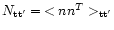
A&A 374, 358-370 (2001)
DOI: 10.1051/0004-6361:20010692
MAPCUMBA: A fast iterative multi-grid map-making algorithm for
CMB experiments
O. Doré1 - R. Teyssier1,2 -
F. R. Bouchet1 - D. Vibert1 - S. Prunet3
1 - Institut d'Astrophysique de Paris, 98bis, Boulevard Arago,
75014 Paris, France
2 - Service d'Astrophysique, DAPNIA, Centre
d'Études de Saclay, 91191 Gif-sur-Yvette, France
3 - CITA,
McLennan Labs, 60 St George Street, Toronto, ON M5S 3H8, Canada
Received 21 December 2000 / Accepted 2 May 2001
Abstract
The data analysis of current Cosmic Microwave Background
(CMB) experiments like BOOMERanG or MAXIMA poses severe challenges
which already stretch the limits of current (super-) computer
capabilities, if brute force methods are used. In this paper we present
a practical solution for the optimal map making problem which can be
used directly for next generation CMB experiments like ARCHEOPS and
TopHat, and can probably be extended relatively easily to the full
PLANCK case. This solution is based on an iterative multi-grid Jacobi
algorithm which is both fast and memory sparing. Indeed, if there are
 data points along the one dimensional timeline to analyse,
the number of operations is of
data points along the one dimensional timeline to analyse,
the number of operations is of
 and the memory requirement is
 .
Timing and accuracy issues have been analysed on
simulated ARCHEOPS and TopHat data, and we discuss as well the issue
of the joint evaluation of the signal and noise statistical
properties.
.
Timing and accuracy issues have been analysed on
simulated ARCHEOPS and TopHat data, and we discuss as well the issue
of the joint evaluation of the signal and noise statistical
properties.
Key words: methods: data analysis - cosmic microwave background
As cosmology enters the era of "precision'', it enters simultaneously
the era of massive data sets. This has in turn showed the need for new
data processing algorithms. Present and future CMB experiments in
particular face some new and interesting challenges (Bond et al. 1999). If
we accept the now classical point of view of a four steps data
analysis pipeline: i) from time-ordered data (TOD) to maps of
the sky at a given frequency, ii) from frequency maps to (among
others) a temperature map, iii) from a temperature map to its power
spectrum  ,
iv) from the power spectrum to cosmological
parameters and characteristics of the primordial spectrum of
fluctuation, the ultimate quantities to be measured in a given
model. The work we are presenting focuses on the first of these issues,
namely the map-making step.
,
iv) from the power spectrum to cosmological
parameters and characteristics of the primordial spectrum of
fluctuation, the ultimate quantities to be measured in a given
model. The work we are presenting focuses on the first of these issues,
namely the map-making step.
Up to the most recent experiments, maps could be made by a brute force
approach that aims to solve directly a large linear problem by direct
matrix inversion. Nevertheless the size of the problem, and the
required computing power, grows as
 ,
and the limits of this kind of method have now been reached
(Borrill 2000) (even if the
,
and the limits of this kind of method have now been reached
(Borrill 2000) (even if the
 scaling of a
preconditioned conjuguate gradient is actually the appropirate scaling
for map-making only). Whereas the most efficient development in this massive
computing approach, i.e. the MADCAP package (Borrill 1999) has been
applied to the recent BOOMERanG and MAXIMA experiments
(de Bernardis et al. 2000; Hanany et al. 2000) some faster and less consuming solutions
based on iterative inversion algorithms have now been developed and
applied too (Prunet et al. 2000). This is in the same spirit as
(Wright et al. 1996), and we definitely follow this latter approach.
scaling of a
preconditioned conjuguate gradient is actually the appropirate scaling
for map-making only). Whereas the most efficient development in this massive
computing approach, i.e. the MADCAP package (Borrill 1999) has been
applied to the recent BOOMERanG and MAXIMA experiments
(de Bernardis et al. 2000; Hanany et al. 2000) some faster and less consuming solutions
based on iterative inversion algorithms have now been developed and
applied too (Prunet et al. 2000). This is in the same spirit as
(Wright et al. 1996), and we definitely follow this latter approach.
Design goals are to use memory sparingly by handling only columns or
rows instead of full matrixes and to increase speed by minimising the
number of iterations required to reach the sought convergence of the
iterative scheme. We fulfill these goals by an iterative multi-grid
Jacobi algorithm. As recalled below, an optimal method involves using
the noise power spectrum. We have thus investigated the
possibility of a joint noise (and signal) evaluation using this algorithm.
Section 2 presents in detail the method and its
implementation, while Sect. 3 demonstrates its
capabilities by using simulations of two on-going balloon CMB
experiments, ARCHEOPS![[*]](/icons/foot_motif.gif) (Benoit et al.
2000)
and TopHat. The results are
discussed in Sect. 4, together with the problem of
the evaluation of the noise properties, as well as possible extensions.
(Benoit et al.
2000)
and TopHat. The results are
discussed in Sect. 4, together with the problem of
the evaluation of the noise properties, as well as possible extensions.
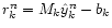
2 The method
The relation between the sky map we seek and the observed data stream
may be cast as a linear algebra system (Wright et al. 1996;
Tegmark 1997; Bond et al. 1998). Let  and
and  indices denote quantities in the temporal and spatial
domains, and group as a data vector,
indices denote quantities in the temporal and spatial
domains, and group as a data vector,  ,
and a noise vector the
temporal stream of collected data and the detector noise stream, both of
dimension
.
We then have
,
and a noise vector the
temporal stream of collected data and the detector noise stream, both of
dimension
.
We then have
 |
(1) |
where
 is the signal vector given by the observation of
the unknown pixelised sky map,
is the signal vector given by the observation of
the unknown pixelised sky map,  ,
which has been arranged as a
vector of dimension
,
which has been arranged as a
vector of dimension
 .
The
.
The
 "observation'' matrix A therefore encompasses the
scanning strategy and the beam pattern of the detector.
"observation'' matrix A therefore encompasses the
scanning strategy and the beam pattern of the detector.
In the following, we restrict the discussion to the case when the beam pattern is
symmetrical. We can therefore take
to be a map of the sky which
has already been convolved with the beam pattern, and A only
describes how this sky is being scanned. For the total power measurement
(i.e. non-differential measurement) we are interested in here, the
observation matrix A then has a single non-zero element per row,
which can be set to one if d and x are expressed in the same
units. The model of the measurement is then quite transparent: each
temporal datum is the sum of the pixel value to which the detector is
pointing plus the detector noise.
The map-making step then amounts to best solve for x given d (and some
properties of the noise). We shall seek a linear estimator of ,
 |
(2) |
To motivate a particular choice of the
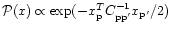
 matrix W, a Bayesian approach is convenient.
Indeed we are seeking the optimal solution to this inversion problem which
maximises the probability of a deduced set of theory parameters (here the map
)
given our data ()
by maximising
matrix W, a Bayesian approach is convenient.
Indeed we are seeking the optimal solution to this inversion problem which
maximises the probability of a deduced set of theory parameters (here the map
)
given our data ()
by maximising
 .
Bayes'
theorem simply states that
.
Bayes'
theorem simply states that
 |
(3) |
If we do not assume any theoretical prior, then
x follows a uniform distribution as well as d. Therefore,
If we further assume that the noise is Gaussian, we can write
where
 is the noise covariance matrix.
In this particular case, maximising
amounts to
find the least square solution which was used to analyse the COBE data
(Jansen & Gulkis 1992),
is the noise covariance matrix.
In this particular case, maximising
amounts to
find the least square solution which was used to analyse the COBE data
(Jansen & Gulkis 1992),
![\begin{displaymath}
W = \left[A^T N^{-1} A\right]^{-1} A^T N^{-1}\: .
\end{displaymath}](/articles/aa/full/2001/28/aa10596/img34.gif) |
(8) |
In this paper we will actually deal only with this
estimator. Nevertheless as a next iteration in the analysis process,
we could incorporate various theoretical priors by making
 more explicit. For example, it is often assumed
a Gaussian prior for the theory, i.e.
more explicit. For example, it is often assumed
a Gaussian prior for the theory, i.e.
 where
where
 is the
signal covariance matrix. In that case the particular solution
turns out to be the Wiener filtering solution
(Zaroubi et al. 1995; Bouchet & Gispert 1996;
Tegmark & Efstathiou 1996; Bouchet & Gispert 1998):
is the
signal covariance matrix. In that case the particular solution
turns out to be the Wiener filtering solution
(Zaroubi et al. 1995; Bouchet & Gispert 1996;
Tegmark & Efstathiou 1996; Bouchet & Gispert 1998):
![\begin{displaymath}W = \left[ C^{-1} + A^T N^{-1} A \right]^{-1} A^T N^{-1}\ .
\end{displaymath}](/articles/aa/full/2001/28/aa10596/img38.gif) |
(9) |
However this solution may always be obtained by a further (Wiener)
filtering of the priorless maximum likelihood solution, and we do not consider it further.
The prior-less solution demonstrates that as long as the (Gaussian)
instrumental noise is not white, a simple averaging (co-addition) of
all the data points corresponding to a given sky pixel is not
optimal. If the noise exhibits some temporal correlations, as induced
for instance by a low-frequency 1/f behavior of the noise spectrum
which prevails in most CMB experiments, one has to take into account
the full time correlation structure of the noise. Additionally, this
expression demonstrates that even if the noise has a simple time
structure, the scanning strategy generically induces a non-trivial
correlation matrix
![$\left[ A^T N^{-1} A\right]^{-1}$](/articles/aa/full/2001/28/aa10596/img39.gif) of the noise map.
of the noise map.
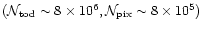
Even if the problem is well posed formally, a quick look at the
orders of magnitude shows that the actual finding of a solution is a non
trivial task. Indeed, a brute force method aiming at inverting the full
matrix
![$\left[ A^T N^{-1} A\right]^{-1} \displaystyle$](/articles/aa/full/2001/28/aa10596/img40.gif) ,
an operation
scaling as
,
an operation
scaling as
 ,
is already hardly
tractable for present long duration balloon flights as MAXIMA,
BOOMERanG, ARCHEOPS or TopHat where
,
is already hardly
tractable for present long duration balloon flights as MAXIMA,
BOOMERanG, ARCHEOPS or TopHat where
 and
and
 .
It appears totally impractical for
PLANCK since for a single detector (amid 10s)
.
It appears totally impractical for
PLANCK since for a single detector (amid 10s)
 and
and
 !
!
One possibility may be to take advantage of specific scanning
strategies, and actually solve the inverse of the convolution problem
as detailed in Wandelt & Gorski (2000). This amounts to deducing the
map coefficients
 in the spherical harmonic basis through a
rotation of a Fourier decomposition of the observed data. The map
will then be a simple visualisation device, while the
would
be used directly for a component separation (as in
Bouchet & Gispert 1996; Tegmark & Efstathiou 1996; Bouchet &
Gispert 1998) and the CMB power spectrum estimate. While potentially
very interesting, this approach will not be generally applicable (at
least efficiently), and we now turn to a practical (general) solution
of Eq. (2) by iterative means.
in the spherical harmonic basis through a
rotation of a Fourier decomposition of the observed data. The map
will then be a simple visualisation device, while the
would
be used directly for a component separation (as in
Bouchet & Gispert 1996; Tegmark & Efstathiou 1996; Bouchet &
Gispert 1998) and the CMB power spectrum estimate. While potentially
very interesting, this approach will not be generally applicable (at
least efficiently), and we now turn to a practical (general) solution
of Eq. (2) by iterative means.
We solve the map-making problem by adapting to our particular case the
general "multi-grid method'' (Press et al. 1992). Multi-grid methods are
commonly used to speed up the convergence of a traditional relaxation
method (in our case the Jacobi method, as in Prunet et al. 2000 defined at
resolution
 (see below). A set of recursively defined
coarser grids (
(see below). A set of recursively defined
coarser grids (
 )
are used as temporary
computational space, in order to increase the convergence rate of the
relaxation process. To be fully profitable, this algorithm implies
for each resolution both a rebinning in space (resolution change) and
in time (resampling).
)
are used as temporary
computational space, in order to increase the convergence rate of the
relaxation process. To be fully profitable, this algorithm implies
for each resolution both a rebinning in space (resolution change) and
in time (resampling).
In this paper, we use the HEALPix pixelisation of the sphere
(Górski et al. 1998). In this scheme, the sphere is covered by 12 basic
quadrilaterals, further divided recursively into pixels of equal
area. The map resolution is labeled by
 :
the number of
pixels along the side of one basic quadrilateral. Hence,
:
the number of
pixels along the side of one basic quadrilateral. Hence,
 means that the sphere is covered by 12 large pixels only. The
number of pixels is given by
means that the sphere is covered by 12 large pixels only. The
number of pixels is given by
 .
.
 corresponds to a pixel size of 13.7 arcmin. For practical
reasons, we need to define the resolution k of a HEALPix
map as
corresponds to a pixel size of 13.7 arcmin. For practical
reasons, we need to define the resolution k of a HEALPix
map as
 |
(10) |
The "nested''pixel numbering scheme of HEALPix (Górski et al. 1998) allows an
easy implementation of the coarsening (
 )
and refining (
)
and refining (
 )
operators that
we use intensively in our multigrid scheme.
)
operators that
we use intensively in our multigrid scheme.
We now discuss the details of our implementation and of the exact
system we solve, the way we solve it and the actual steps of the multi-grid algorithm.
The timeline is given by
 where
where
 is the sky map at "infinite'' resolution
(
is the sky map at "infinite'' resolution
( in our notations). We aim at solving for the optimal map
 at a given finite spatial resolution k using
 |
(11) |
where Ak is the "observation'' operator (from spatial to
temporal domain) and AkT is the "projection'' operator
(from temporal to spatial domain). In a noise-free experiment, the
optimal map would be straightforwardly given by the co-added map
(introducing the "co-addition'' operator Pk)
 |
(12) |
In order to check the accuracy of this trivial noise-free map making,
it is natural to compute the residual in the time domain with n=0
 |
(13) |
which will be non-zero in practice, as soon as one works with
finite spatial resolution. We call this residual the pixelisation noise. Since we assume here that the instrumental
beam is symmetric, the sky map is considered as the true sky
convolved by, say, a Gaussian beam of angular diameter
 .
This introduces a low-pass spatial filter in the problem.
In other words, as the resolution increases, the pixelisation noise
should decrease towards zero. We evaluate the order of magnitude of the
pixelisation noise this way:
.
This introduces a low-pass spatial filter in the problem.
In other words, as the resolution increases, the pixelisation noise
should decrease towards zero. We evaluate the order of magnitude of the
pixelisation noise this way:
where
 is the typical pixel width at resolution
k and
is the typical pixel width at resolution
k and
 is the signal norm. This formula is an evaluation
of the maximal variation of the signal visible on a beam size. The
norms used in the above formula can be either the maximum over
the time line (a very strong constraint) or the variance over the
time line (a weaker constraint). Since the pixelisation noise is
strongly correlated with the sky signal (the more the
signal varies, the higher this noise), point sources or Galaxy
crossings are potential candidates for large and localised bursts
of pixelisation noise. The correct working resolution
is the signal norm. This formula is an evaluation
of the maximal variation of the signal visible on a beam size. The
norms used in the above formula can be either the maximum over
the time line (a very strong constraint) or the variance over the
time line (a weaker constraint). Since the pixelisation noise is
strongly correlated with the sky signal (the more the
signal varies, the higher this noise), point sources or Galaxy
crossings are potential candidates for large and localised bursts
of pixelisation noise. The correct working resolution  is set by requiring that the pixelisation noise remains low
compared to the actual instrumental noise, or equivalently
is set by requiring that the pixelisation noise remains low
compared to the actual instrumental noise, or equivalently
 |
(16) |
Note however that the pixelisation noise is strongly non Gaussian (point sources or
Galaxy crossings) and can be always considered as a potential source
of residual stripes in the final maps.
2.2.2 The basic relaxation method: An approximate Jacobi solver
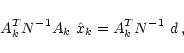
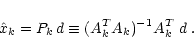
Instead of solving for  we perform the change of
variable
we perform the change of
variable
 |
(17) |
and solve instead for  which obeys
 |
(18) |
where we have multiplied each side of Eq. (11) by
(AT A)-1, the pixel hit counter. From now on, we also assume
that the noise in the timestream is stationary and that its covariance
matrix is normalised so that
 .
The previous
change of variable allows us to subtract the sky signal from the data:
since we have chosen a resolution high enough to neglect the pixelisation noise, we have
indeed
.
The previous
change of variable allows us to subtract the sky signal from the data:
since we have chosen a resolution high enough to neglect the pixelisation noise, we have
indeed
 and,
consequently,
and,
consequently,
 .
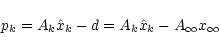
The map making consists of
two steps: first to compute a simple co-added map from the time line,
and second, to solve Eq. (18) for the stripes map .
The
final optimal map is obtained by adding these two maps.
.
The map making consists of
two steps: first to compute a simple co-added map from the time line,
and second, to solve Eq. (18) for the stripes map .
The
final optimal map is obtained by adding these two maps.
It is worth mentioning that the stripes map is completely
independent of the sky signal, as soon as the pixelisation noise
can be ignored. It depends only on the scanning strategy through the
matrix A and on the noise characteristics through the matrix N.
Even if in principle this change of variable is irrelevant since it
does not change the matrix to be inverted, it does so in practice
since d-A P d is free from the fast variations of d (up to the
pixelisation noise), as e.g. the Galaxy crossings, which are
numerically damaging to the quality of the inversion.
To solve for Eq. (18), we follow the ideas of Prunet
et al. (2000) and apply an approximate Jacobi relaxation scheme.
The Jacobi method consists in the following relaxation step to
solve for our problem
 |
(19) |
where D is the diagonal part of the matrix M and R is the residual
matrix
R = I - D-1M. Computing the diagonal elements of
M=P N-1A is rather prohibitive. The idea of Prunet et al.
(2000) is to approximate
 by neglecting the
off-diagonal elements of N-1. The residual matrix then simplifies
greatly and writes
by neglecting the
off-diagonal elements of N-1. The residual matrix then simplifies
greatly and writes
 |
(20) |
The approximate Jacobi relaxation step is therefore defined as
 |
(21) |
One clearly sees that if this iterative scheme converges, it is
towards the full solution of Eq. (18). To perform these
successive steps, it is extremely fruitful to remember the assumed
stationarity of the noise. Indeed whereas this assumption implies a circulant
noise covariance matrix in real space, it translates in Fourier space in the
diagonality of the noise covariance matrix. This is naturally another
formulation of the convolution theorem, since a stationary matrix
acts on a vector as a convolution, and a diagonal matrix acts as a
simple vector product, thus a convolution in real space is
translated as a product in Fourier space. The point is that the
manipulation of the matrix N-1 is considerably lighter and
will henceforth be performed in Fourier space. Applying the matrix
R to a map reduces then to the following operations in order to:
- 1.
- "Observe'' the previous stripes map
 ;
;
- 2.
- Fourier transform the resulting data stream;
- 3.
- Apply the low-pass filter
W=I-N-1;
- 4.
- Inverse Fourier transform back to real space;
- 5.
- Co-add the resulting data stream into the map
 .
.
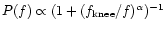
Assuming that the normalised noise power spectrum can be
approximated by
 ,
the low-pass filter associated to each
relaxation step is given by
,
the low-pass filter associated to each
relaxation step is given by
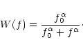 |
(22) |
Since both A and P are norm-preserving operators, the norm of
the increment
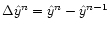 between step n and n+1 decreases as
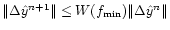 ,
where
,
where  is a minimal frequency in the problem. Since
 ,
we
see that the approximate Jacobi relaxation scheme will converge in
every case, which is good news. On the other hand, since
,
we
see that the approximate Jacobi relaxation scheme will converge in
every case, which is good news. On the other hand, since
 ,
the actual convergence rate of the scheme is likely to be
very, very slow, which is bad news (cf. Fig. 6 for
a graphical illustration).
The fact that this algorithm is robust, but dramatically slow is a
well-known property of the Jacobi method. The multi-grid method is
also well known to solve this convergence speed problem. Note that
if the convergence is reached, the solution we get is the optimal
solution, i.e. similar to the one that would be obtained by a full
matrix inversion up to round-up errors.
,
the actual convergence rate of the scheme is likely to be
very, very slow, which is bad news (cf. Fig. 6 for
a graphical illustration).
The fact that this algorithm is robust, but dramatically slow is a
well-known property of the Jacobi method. The multi-grid method is
also well known to solve this convergence speed problem. Note that
if the convergence is reached, the solution we get is the optimal
solution, i.e. similar to the one that would be obtained by a full
matrix inversion up to round-up errors.
The multi-grid method for solving linear problems is described in
great detail in Press et al. (1992). At each relaxation step at level
 ,
our target resolution, we can define the error
,
our target resolution, we can define the error
 and the residual
 .
Both are related through
.
Both are related through
 |
(23) |
If we are able to solve exactly for Eq. (23), the
overall problem is solved. The idea of the multi-grid algorithm is
to solve approximately for Eq. (23) using a coarser
"grid'' at resolution k-1, where the relaxation scheme should
converge faster. We thus need to define a fine-to-coarse operator, in
order to define the new problem on the coarse grid and solve for
it. We also need a coarse-to-fine operator in order to inject the
solution onto the fine grid. The approximation to the error
ekn is finally added to the solution. The coarse grid
solver is usually applied after a few iterations on the fine level
have been performed (in practice we perform 3 to 5 iterations).
Naturally, since the solution to the problem on the coarse level
relies also on the same relaxation scheme, it can be itself
accelerated using an even coarser grid. This naturally leads to a
recursive approach of the problem.
We defined our fine-to-coarse operator to be an averaging of the values of
the 4 fine pixels contained in each coarse pixel. The
coarse-to-fine operator is just a straight injection of the value
of the coarse pixel into the 4 fine pixels. The most important issue
is the temporal rebinning of the data stream, since the speed of the
iterative scheme at a given level is actually set by the two Fourier
transforms. We performed that resampling by simply taking one point
out of two each time we go up one level. At the lower resolutions, this
reduction is such that the iteration cost is negligible when
compared to that at higher k; it allows fast enough iterations
that full convergence may be reached. In practice, we choose a minimal level
k=3 defined by
 and iterate a few hundred times to
reach exact convergence.
and iterate a few hundred times to
reach exact convergence.
Finally, the navigation through levels allows several options to be
taken. Either we go up and down through all the levels successively
(the so-called "V-cycle'') or we follow more intricate paths (e.g. the
"W-cycle'' where at a given level we go down and up all the
lower levels before going up and vice-versa). Since it turns out
that levels are relatively disconnected in the sense that the scales
well solved at a given resolution are only slightly affected by the
solution at a higher level, the "V-cycle'' is appropriate and is
the solution we adopt in the two following configurations.
We now aim at demonstrating the capabilities of this algorithm with
simulated data whose characteristics are inspired by those of the ARCHEOPS and
TopHat experiments.
The ARCHEOPS and TopHat experiments are very similar with respect to
their scanning strategy. Indeed both use a telescope that simply spins
at a constant rate (respectively 3 and 4 RPM) about its vertical
axis. Thus due to Earth rotation the sky coverage of both is
performed through scan circles whose axis slowly drifts on the
sky. Nevertheless, because of the different launch points
(respectively on the Arctic circle (Kiruna, Sweden) and in Antarctica
(McMurdo)) and their different telescope axis elevation (respectively
 41
41 or 12)
they do not have the same sky coverage.
or 12)
they do not have the same sky coverage.
Otherwise the two experiments do not use the same bolometers
technology, the same bands or have the same number of
bolometers. But even if we try to be fairly realistic, our goal though
is not to compare their respective performances but rather to
demonstrate two applications of our technique in different
settings. We then simulate for each a data stream of 24 hrs
duration with respectively a sampling frequency of 171and
 .
The TODs contain realistic CMB and Galactic
signal for a band at
.
The TODs contain realistic CMB and Galactic
signal for a band at
 .
Note that this is a one day
data stream for TopHat (out of 10 expected) and that this frequency
choice is more appropriate for ARCHEOPS than for TopHat (whose
equivalent band is around
.
Note that this is a one day
data stream for TopHat (out of 10 expected) and that this frequency
choice is more appropriate for ARCHEOPS than for TopHat (whose
equivalent band is around
 ), but this is realistic
enough for our purpose. We generated a Gaussian noise time stream with
the following power spectrum:
), but this is realistic
enough for our purpose. We generated a Gaussian noise time stream with
the following power spectrum:
 with
with
 and
and
 ,
and
,
and
 and 1. The noise amplitude per
channel is chosen so that it corresponds for ARCHEOPS (24 hours) and
TopHat (10 days of flight)
to
and 1. The noise amplitude per
channel is chosen so that it corresponds for ARCHEOPS (24 hours) and
TopHat (10 days of flight)
to
 on average per 20' pixel, with a beam
FWHM of 10'/20'. Note that we restrict ourselves arbitrarily to
shorter timeline that the method could handle in principle for time saving reason
only. In principle the method could possibly deal with the full timeline at
once (see below for memory issue discussion in Sect. 4.2)
for the two experiments but we restrict ourselves on purpose to mere demonstrative examples.
on average per 20' pixel, with a beam
FWHM of 10'/20'. Note that we restrict ourselves arbitrarily to
shorter timeline that the method could handle in principle for time saving reason
only. In principle the method could possibly deal with the full timeline at
once (see below for memory issue discussion in Sect. 4.2)
for the two experiments but we restrict ourselves on purpose to mere demonstrative examples.
We introduced 5 distinct levels of resolution defined by their
parameter in the HEALPix package (Górski et al. 1998). The
highest resolution level is imposed by the pixelisation noise level
requirement (Sect. 2.2.3) to
(pixel size
13.7') whereas the lowest one is
(pixel size
7.3). Therefore these two configurations each offer an interesting
test since they differ by the sky coverage and the noise power
spectrum. We iterate 3 times at each level except at the lowest one
where we iterate 100 times.
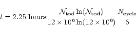
The algorithm is equally efficient in both situations. Whereas for ARCHEOPS
(whose timeline is longer due to the higher sampling frequency) it took
2.25 hours on a SGI ORIGIN 2000 single processor, it took around 1.5 hours for the TopHat daily data stream.
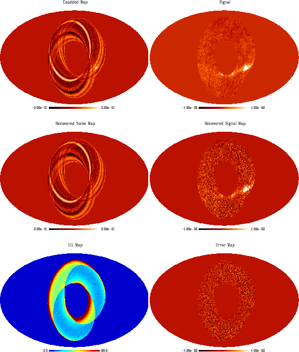
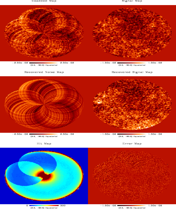
In Figs. 1 and 2 we depict from top to
bottom and from left to right the initial co-added data, the
reconstructed noise map, the hit map, i.e. the number of hits per pixel
at the highest resolution, the initial signal map as well as the
reconstructed signal map and the error map. We see that the destriping
is excellent in both situations and the signal maps recovered only
contain an apparently isotropic noise. We note the natural correlation
between the error map and the hit map. Finally, we stress that
no previous filtering at all has been applied.
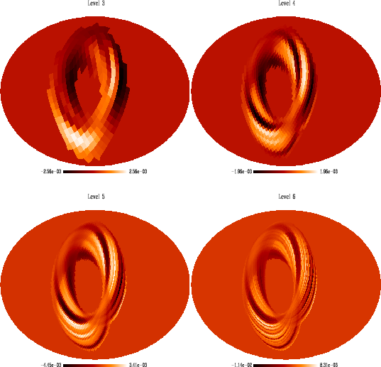
As an illustration of how our multi-grid work method works, Fig. 3
shows how the noise map is reconstructed at various
scales.
 |
Figure 1:
Simulated ARCHEOPS Kiruna flight: from top to bottom and
from left to right, the co-added map and the input Galactic + CMB
signal map, the reconstructed noise (stripes) and signal maps, the hit
count and the error map (Arbitrary unit). The fact that the coverage
is not fully symmetrical is due to the fact that we considered
slightly less than
24 hr. Mollweide projection with pixels
of 13.7' (HEALPix
). Arbitrary units. |
| Open with DEXTER |
 |
Figure 2:
Simulated TopHat one day flight: from top to bottom and from
left to right, the co-added map and the input CMB + Galaxy signal map,
the reconstructed noise (or stripes) and signal map, the hit count and
error map. The fact that the coverage is not fully symmetrical is due
to the fact that we consider only
18.2 rm hr of
flight. Gnomonic projection with pixel of 13.7' (HEALPix
). Note that the slight visible striping is correlated to the
incomplete rotation pattern that we arbitrary chose. Arbitrary units. |
| Open with DEXTER |
 |
Figure 3:
Multi-grid noise map recovery: in this plot we show in the
ARCHEOPS Kiruna case how the noise map is reconstructed at various
levels, corresponding respectively to
 . . |
| Open with DEXTER |
In this section, we present some tests we carried out to validate our
method. First, as was stated below, as soon as the iterative algorithm
converges, the solution is by construction the optimal solution,
similar to the one that would be obtained by the full matrix
inversion. As a criterium for convergence we required the 2-norm of
residuals to be of the order of the machine accuracy.
We initially have a Gaussian random noise stream fully characterised
by its power spectrum. Therefore an important test is to check wether
the deduced noise stream (by "observing'' the stripe map, see
Sect. 4.3 for further details) is Gaussian and
has the same power spectrum. In Fig. 4 we ensure that the
evaluated noise time stream is indeed Gaussian. As depicted in Fig. 5,
where we plot in the ARCHEOPS case both the analytical
expression of the spectrum according to which we generate the timeline
and its recovered form, the agreement is excellent. We recall that we
assumed at the beginning a perfect knowledge of the noise in order to
define the filters. This is naturally unrealistic but the issue of
noise evaluation is discussed in Sect. 4.3 below. We
plotted as well the probability distribution function (PDF) of the
final error map, i.e. the recovered noisy signal map minus the input
signal map (Fig. 4). This PDF is well fitted by a Gaussian whose
parameters are given in Fig. 4. The PDF of the error map
displays some non-Gaussian wings. Let us recall that this is no
surprise here because of the non-uniform sky coverage as well as the
slight residual striping, both due to the non-ideal scanning
strategy, i.e. that produces a non-uniform white noise in pixel space.
Another particularly important test consists in checking the
absence of correlation between the recovered noise map and the
initial signal map. We could not find any which is no surprise since
we are iterating on a noise map (see Sect. 2.2.2) which does not contain any signal up
to the pixelisation noise, that is ensured to be negligible with regards to the
instrumental noise by choice of the resolution
(see Sect. 2.2.1).
![\begin{figure}
\par\includegraphics[angle=90,width=8.3cm]{AA10596f4a.ps}\par\includegraphics[angle=90,width=8.3cm]{AA10596f4b.ps}
\end{figure}](/articles/aa/full/2001/28/aa10596/Timg110.gif) |
Figure 4:
In the TopHat case we plot from top to bottom the recovered
probability distribution function of the noise stream evaluated along
the timeline as well as the error map PDF. In these two cases a fit to
a Gaussian has been performed whose parameters are written inside the
figures. No significant departure from a Gaussian distribution are detected. The
arbitrary units are the same as the ones used for the previously shown
maps. |
| Open with DEXTER |
![\begin{figure}
\par\includegraphics[angle=90,width=8.5cm]{AA10596f5a.ps}\par\includegraphics[angle=90,width=8.5cm]{AA10596f5b.ps}
\end{figure}](/articles/aa/full/2001/28/aa10596/Timg111.gif) |
Figure 5:
Recovery of the noise power spectrum in the Archeops case
(top: linear x-axis, bottom: log x-axis): the red thin dashed line
shows the initial analytic noise power spectrum used to generate the
input noise stream and the blue thick line denotes the recovered one
after 6 iterations. The recovered one has been binned as described in
Sect. 4.3 and both have been normalised so that the
white high frequency noise spectrum is equal to one. The agreement is
obviously very good. No apparent bias is visible. Note that a perfect
noise power spectrum prior knowledge has been used in this
application. |
| Open with DEXTER |
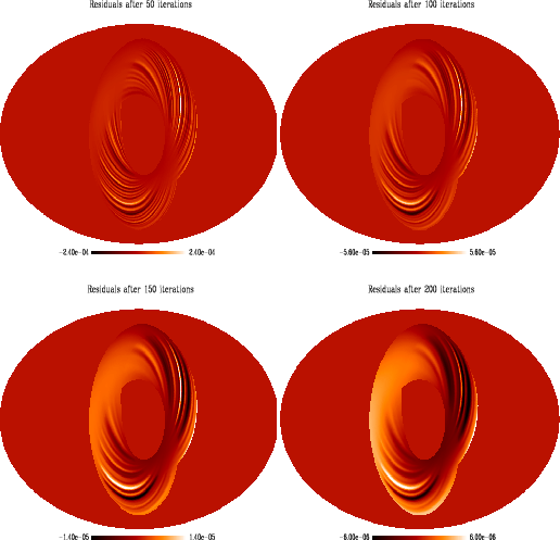
The efficiency of such a method can be intuitively understood. Indeed,
although the Jacobi method is known to converge very safely, it suffers
intrinsically from a very slow convergence for large-scale
correlations (which originate mainly in the off diagonal terms of the
matrix to be inverted) (Press et al. 1992). This is illustrated in Fig. 6:
we show the maps of residuals after solving this
system using a standard Jacobi method on simulated data with
50, 100, 150, and 200 iterations. We used the same simulation
and therefore the same sky coverage. Obviously the largest structures
are the slowest to converge (implying observed large scale residual
patterns). As a consequence it seems very natural to help the
convergence by solving the problem at larger scales. Whereas
large-scale structures will not be affected by a scale change, smaller
structures will converge faster.
We have found that this multi-grid algorithm translates naturally in
a speed up factor greater than 10 as compared to a standard Jacobi
method. This is illustrated in Fig. 7 where we
plotted the evolution of the 2-norm of residuals for the two methods
in terms of the number of iterations in "cycle units". One cycle
corresponds to 8 iterations at level
for a standard
Jacobi method whereas it incorporates additionally going up and down all
the lowest levels in the multi-grid case. Thus the cycle timing is not
exactly the same but the difference is negligible since the limiting
stages are definitely the iterations performed at maximum
resolution. Note the fact that the efficiency of the multi-grid method
allows us to solve exactly the system up to the 4-byte machine accuracy
(small rebounds at the bottom of the curve) in approximately
135 mn for
 on a SGI ORIGIN 2000 single
processor. Note also that this ultimate convergence is definitely an
overkill and is somewhat artificial for current CMB
experiments. Indeed, residuals with a norm smaller than noise per
pixel are meaningless. Since the limiting stages are the FFT's at the higher levels, this
algorithm scales as
.
In its current implementation, a rough
scaling could be written this way:
on a SGI ORIGIN 2000 single
processor. Note also that this ultimate convergence is definitely an
overkill and is somewhat artificial for current CMB
experiments. Indeed, residuals with a norm smaller than noise per
pixel are meaningless. Since the limiting stages are the FFT's at the higher levels, this
algorithm scales as
.
In its current implementation, a rough
scaling could be written this way:
 |
(24) |
(note that we expect some further speed-up by reducing the number of
operations at level max and eventually using a faster FFT).
 |
Figure 6:
Residual map after 50, 100, 150 and 200 iterations of a
standard Jacobi method. This has been performed on simulated data
for one bolometer with a nominal noise level. The sky coverage is
that of ARCHEOPS coming Kiruna flight. The residual large scale
patterns illustrate the difficulties the standard Jacobi method faces
to converge. The stripes free area are the ones of scan crossing (see
the hit map in Fig. 1). |
| Open with DEXTER |
In terms of memory storage (RAM) it scales naturally as
since one crucial feature of this
iterative method is to handle only vectors and never an explicit
matrix. Typically one single timeline size object is needed at any one
time in memory. Since projection and observation operations are formally independent of the
number of pixels, the scaling in
is definitely
subdominant.
In terms of speed and efficiency, this method should well compare
to a more obvious iterative inversion scheme such as preconditioned conjuguate
gradient technique. The latter also has a scaling dominated by FFT as
(Natoli et al.). A precise
study comparing the relevant pre-factors but also discussing
convergence criteria will be the object of a forthcoming paper.
The estimation of the statistical properties of the noise in the
timestream is an issue of paramount importance for map-making. Indeed,
whereas till now we have assumed a perfect prior knowledge of the
noise power spectrum in order to define the filters, it might not be
that easy in practice since we cannot separate the signal from the
noise. We will therefore aim at making a joint estimation of the
signal and the noise. This has been pioneered recently by Ferreira &
Jaffe (2000) and implemented independently by Prunet et al. (2000). The
latter implementation is rather straightforward in our particular case
since it just implies reevaluating the filters after a number of
iterations, given the (current) estimation of the signal map and thus
of the signal data stream. Nevertheless its non-obvious convergence
properties have to be studied carefully through simulations. Making
use of (17) our evaluation of the noise timeline
 at the nth iteration and at level max is
 |
(25) |
Then we
compute its spectrum and (re-) define the required filters. We then go
through several multi-grid cycles (5 in the above demonstrated case)
before re-evaluating the noise stream. Very few evaluations of the
noise are needed before getting a converged power spectrum (around 2).
In such an implementation, no noise priors at all are
assumed. This is illustrated on one particular worked out example in
the case of a 4 hours ARCHEOPS like flight (more detailed
considerations will be discussed elsewhere). To reduce the number
of degrees of freedom we bin the evaluated noise power spectrum using
a constant logarithmic binning (
 in our case) for
 and a constant linear binning
(
and a constant linear binning
(
 in our case) for higher
frequency. Figure 8 shows the genuine and evaluated noise power
spectrum. The initial noise power spectrum was a realistic one
in our case) for higher
frequency. Figure 8 shows the genuine and evaluated noise power
spectrum. The initial noise power spectrum was a realistic one
 to which we
added some small perturbations (the two visible bumps) to test the
method. Note the small bias around the telescope spin frequency at
to which we
added some small perturbations (the two visible bumps) to test the
method. Note the small bias around the telescope spin frequency at
 :
this is illustrative of the
difficulties we fundamentally face to separate signal and noise at
this particular frequency through Eq. (17). Naturally, this
bias was not present in the case demonstrated in Fig. 5
where we assumed a prior knowledge of the spectrum. This possible bias
forced us to work with a coarser binning (
:
this is illustrative of the
difficulties we fundamentally face to separate signal and noise at
this particular frequency through Eq. (17). Naturally, this
bias was not present in the case demonstrated in Fig. 5
where we assumed a prior knowledge of the spectrum. This possible bias
forced us to work with a coarser binning (
 )
in the
1/f part of the spectrum until the convergence is reached, i.e. we
evaluate the noise power spectrum with the previously mentioned
binning only at the last step. Proceeding this way, the convergence
towards the correct spectrum is both fast (3 noise evaluations) and
stable.
)
in the
1/f part of the spectrum until the convergence is reached, i.e. we
evaluate the noise power spectrum with the previously mentioned
binning only at the last step. Proceeding this way, the convergence
towards the correct spectrum is both fast (3 noise evaluations) and
stable.
Second, the output of any map-making is meaningless without an
evaluation of the map noise covariance matrix
(AT N-1
A)-1. Given such a fast algorithm (and the fact it gives an evaluation of the
power spectrum), it is natural to obtain it through a Monte-Carlo
algorithm fueled by various realizations of the noise timeline
generated using the evaluated power spectrum (in the spirit of Wandelt
et al. 2000). A detailed study will be performed in a future work.
However we investigate here the chance of this approach being
successfull and illustrate it very briefly by a very rough determination (which is in no way an appropriate estimate). To this end we perform a one day TopHat like simulation
including only the CMB signal plus the noise. From this data stream we
obtain an "optimal'' signal map as well as an evaluation of the noise
power spectrum using the previously described algorithm. With the help
of the anafast routine of the HEALPix package we calculate this way a rough
 .
Using the estimated noise power spectrum we
generate 10 realisations of the noise and get consequently 10"optimal'' noise maps. For each of them we measure as before
and average them to obtain
.
Using the estimated noise power spectrum we
generate 10 realisations of the noise and get consequently 10"optimal'' noise maps. For each of them we measure as before
and average them to obtain
 .
In order to
"de-bias'' the signal power spectrum recovered in this way, we
substract
from
.
The power
spectrum obtained in this manner includes as well some spatial
correlations due to weak residual stripping and thus does not
correspond exactly to white noise (at least in the low
.
In order to
"de-bias'' the signal power spectrum recovered in this way, we
substract
from
.
The power
spectrum obtained in this manner includes as well some spatial
correlations due to weak residual stripping and thus does not
correspond exactly to white noise (at least in the low  part). For the
sake of comparison we compute the power spectrum of the input signal
measured the same way,
part). For the
sake of comparison we compute the power spectrum of the input signal
measured the same way,
 ,
and plotted both
and
,
and plotted both
and
 averaged in linear bands of constant width
 .
The
agreement is obviously very good, as illustrated in Fig. 9.
The error bars take into account both the sampling
induced variance as well as the beam spreading (Knox 1995).
.
The
agreement is obviously very good, as illustrated in Fig. 9.
The error bars take into account both the sampling
induced variance as well as the beam spreading (Knox 1995).
This procedure is in no way an appropriate
measurement
since we are not dealing properly here with the sky coverage induced
window function which triggers some spurious correlations within the
's. We thus do not take into account the full structure of
the map noise covariance matrix. Nevertheless, the efficiency of such a rough method is
encouraging for more detailed implementation and a full handling of
the noise covariance matrix. Note finally that this is a naturally
parallelised task which should therefore be feasible very quickly.
![\begin{figure}
\par\includegraphics[angle=90,width=8.5cm]{AA10596f7.ps}
\end{figure}](/articles/aa/full/2001/28/aa10596/Timg128.gif) |
Figure 7:
The evolution of the 2-norm of residuals with the number of
iterations at level max. Whereas the blue dashed line is standard
iterative Jacobi, the solid red line is the iterative multi-grid
Jacobi method. A full multi-grid cycle incorporates 3 iterations at
level max before going down and up all the levels. The sharp jumps
correspond to the moment when the scheme again reaches max level and
thus benefits from the resolution at lower levels. Note
that the very sharp features after 100 iterations are due to
the fact we reached the 4-byte machine accuracy which is almost out of reach for a
standard iterative method. |
| Open with DEXTER |
![\begin{figure}
\par\includegraphics[angle=90,width=8.5cm]{AA10596f8a.ps}\par\includegraphics[angle=90,width=8.5cm]{AA10596f8b.ps}
\end{figure}](/articles/aa/full/2001/28/aa10596/Timg129.gif) |
Figure 8:
Evaluation of the noise power spectrum (top: linear x-axis,
bottom: log x-axis): the red thin dashed line shows the initial noise
power spectrum obtained from the input noise stream and the blue thick
line denotes the recovered one after 5 iterations. Both have been
smoothed and normalised so that the white high frequency noise
spectrum is equal to one. The agreement is obviously very good. Note
that no noise priors at all have been used in this evaluation. |
| Open with DEXTER |
![\begin{figure}
\par\includegraphics[angle=90,width=8.5cm]{AA10596f9.ps}
\end{figure}](/articles/aa/full/2001/28/aa10596/Timg130.gif) |
Figure 9:
In the case of a one day flight of the TopHat
experiment we perform a very approximate evaluation of the recovered
signal band powers (black) which has to be compared to the input
signal power spectrum (red line). Both have been measured the same way
using the anafast routine of the HEALPix package. These band
powers
 have been performed using a fast
Monte-Carlo evaluation of
(dashed blue line) which
does not correspond exactly to white noise since there remains some
spatial correlations. This in no way constitutes an appropriate
measurement but is an encouraging step towards a full
Monte-Carlo treatment.
have been performed using a fast
Monte-Carlo evaluation of
(dashed blue line) which
does not correspond exactly to white noise since there remains some
spatial correlations. This in no way constitutes an appropriate
measurement but is an encouraging step towards a full
Monte-Carlo treatment. |
| Open with DEXTER |
The application to genuine data could be problematic if our key
hypotheses were not fulfilled. We now turn to their discussion.
Concerning the noise, we assumed that it is Gaussian (in order to derive
our map estimator) and stationary (in order to exploit the diagonality
of its noise covariance matrix in Fourier space). Both hypotheses are reasonable
for a nominal instrumental noise, at least on (sufficiently
long) pieces of timeline. If not, we would have to cut the "bad'' parts and
replace them by a constrained realization of the noise in these
parts. Concerning the signal, no particular assumptions are needed in
the method we are presenting. At this level, we neglected as well the
effect of the non perfect symmetry of the instrumental beam. This
effect should be quantified for a real experiment
(Wu et al. 2000; Doré et al. 2000). Another technical hypothesis is the negligibility of
the pixelisation noise with respect to the instrumental noise but
since this is fully under control of the user it should not be a
problem.
In this paper, we have presented an original fast map-making method
based on a multi-grid Jacobi algorithm. It naturally entails the
possibility of a joint noise/signal estimation. We propose a way to
generate the noise covariance matrix and illustrate its ability on a
simplistic
estimation. The efficiency of this
method has been demonstrated in the case of two coming balloon
experiments, namely ARCHEOPS and TopHat but it naturally has a more
general range of application. This tool should be of natural interest
for Planck and this will be demonstrated elsewhere. Furthermore,
due to the analogy of the formalisms, this should have some
applications as well in the component separation problem.
We hope to apply it very soon to ARCHEOPS data. The FORTRAN
90 code whose results have been presented is available at
http://ulysse.iap.fr/download/mapcumba/.
Acknowledgements
We would like to thank Eric Hivon for fruitful remarks, Lloyd
Knox for stimulating discussions and information on the
TopHat experiment, the developers of the HEALPix (Górski et al. 1998)
package which has considerably eased this work and Julian Borrill, our
referee for suggesting some valuable precisions.
- Benoit, A., et al. 2000, submitted to A&A
In the text
- Bond, J. R., Jaffe, A. H., & Knox, L. 1998,
Phys. Rev. D, 2117
In the text
- Bond, J. R., Crittenden, R. G., Andrew, H., Jaffe, A. H., & Knox, L. 1999, Computing in Science and
Engineering [astro-ph/9903166]
In the text
- Borrill, J. 1999, MADCAP: The Microwave Anisotropy
Dataset Computational Analysis Package Julian Borrill in
Proceeedings of the 5th European SGI/Cray MPP Workshop
[astro-ph/9911389], see also In the text
http://cfpa.berkeley.edu/~borrill/cmb/madcap.html
- Borrill, J. 2000, in proceedings to the
MPA/ESO/MPE Joint Astronomy Conference Mining the sky, Garching
In the text
- Bunn, E. F., Hoffman, Y., & Silk, J. 1996,
ApJ, 464, 1
NASA ADS
-
Bouchet, F. R. 1996, Gispert, AIP Conf. Proc. 348, The mm/sub-mm Foregrounds and Future CMB Space Missions,
ed. E. Dwek
In the text
- Bouchet, F. R., & Gispert, R. 1999,
New Astron., 4, 443B
In the text
NASA ADS
- de Bernardis, P., et al. 2000,
Nature (London) 404, 995
In the text
- Doré, O., Bouchet, F. R., Teyssier,
R., & Vibert, D. 2000, in proceedings to the MPA/ESO/MPE Joint Astronomy
Conference Mining the sky, Garching
In the text
- Ferreira, P. G., & Jaffe,
A. H. 2000, MNRAS, 312, 89
NASA ADS
- Górski, E. K., Hivon, E., & Wandelt, B. D.
1998, in proceedings of the MPA/ESO Garching Conf., ed. A. J. Banday,
K. Sheth, & L. Da Costa In the text
http://www.eso.org/~kgorski/healpix/
- Hanany, S., et al. 2000,
ApJL, submitted [astro-ph/0005123]
In the text
- Jansen, D. J., & Gulkis, S.,
Mapping the Sky with the COBE-DMR, in The Infrared and
Submillimeter Sky after COBE, ed. M. Signore, & C. Dupraz (Dordrecht: Kluwer)
In the text
- Knox, L. 1995, Phys. Rev. D, 52, 4307
In the text
NASA ADS
- Natoli et al., A&A, submitted [astro-ph/0101252]
- Press, W. H., Teukolsky, S. A.,
Vetterling, W. T., & Flannery, B. P. 1992, Numerical Recipes, 2nd ed. (Cambridge
University Press, Cambridge)
In the text
- Prunet, S., Netterfield,
C. B., Hivon, E., & Crill, B. P. 2000, Iterative map-making for scanning experiments,
to be published in the Proceedings of the XXXVth Rencontres de
Moriond, Energy Densities in the Universe (Éditions Frontières)
[astro-ph/0006052]
In the text
- Tegmark, M. 1997, ApJL, 480, L87
In the text
NASA ADS
- Tegmark, M., &
Efstathiou, G. 1996, MNRAS, 281, 1297
In the text
NASA ADS
- Wandelt, B. D., Hivon, E., & Gorski, K. M.,
preprint [astro-ph/0008111]
- Wandelt, B. D., & Gorski, K. M.,
preprint [astro-ph/0008227]
In the text
- Wu, J. H. P., et al., ApJS, in press [astro-ph/0007212]
In the text
- Wright, E. L., Hinshaw, G.,
& Bennett, C. L. 1996, ApJL, 458, 53
In the text
- Wright, E. L., proceeding of the IAS CMB
Workshop [astro-ph/9612006]
- Zaroubi, S., Hoffman, Y., Fisher,
K. B., & Lahav, O. 1995, ApJ, 449, 446
In the text
NASA ADS
Copyright ESO 2001

![\begin{figure}
\par\includegraphics[angle=90,width=8.3cm]{AA10596f4a.ps}\par\includegraphics[angle=90,width=8.3cm]{AA10596f4b.ps}
\end{figure}](/articles/aa/full/2001/28/aa10596/img110.gif)
![\begin{figure}
\par\includegraphics[angle=90,width=8.5cm]{AA10596f5a.ps}\par\includegraphics[angle=90,width=8.5cm]{AA10596f5b.ps}
\end{figure}](/articles/aa/full/2001/28/aa10596/img111.gif)
![\begin{figure}
\par\includegraphics[angle=90,width=8.5cm]{AA10596f7.ps}
\end{figure}](/articles/aa/full/2001/28/aa10596/img128.gif)
![\begin{figure}
\par\includegraphics[angle=90,width=8.5cm]{AA10596f8a.ps}\par\includegraphics[angle=90,width=8.5cm]{AA10596f8b.ps}
\end{figure}](/articles/aa/full/2001/28/aa10596/img129.gif)
![\begin{figure}
\par\includegraphics[angle=90,width=8.5cm]{AA10596f9.ps}
\end{figure}](/articles/aa/full/2001/28/aa10596/img130.gif)