A&A 373, 916-931 (2001)
DOI: 10.1051/0004-6361:20010130
Nonradial adiabatic oscillations of stars
Mode classification of acoustic-gravity waves
I. P. Lopes1,2
1 -
Department of Physics, Nuclear and Astrophysics
Laboratory, Keble Road, Oxford OX1 3RH, UK
2 -
Instituto Superior Técnico, Av. Rovisco Pais,
Centro Multidisciplinar de Astrofísica,
1049-001 Lisboa, Portugal
Received 31 May 2000 /Accepted 17 January 2001
Abstract
The classification scheme of mode oscillations in stars is
investigated mathematically and physically by using a new phase
diagram representation. This technique is presented in order to
study the
basic equation of motion for linear adiabatic nonradial oscillations,
and leads us to obtain an unambiguous scheme classification of
modes. The order number introduced by this classification scheme
only depends on the boundary conditions at the endpoints, the
centre and the surface of the star. Furthermore, this
classification is independent of the number of nodes of
the eigenfunction used to characterize the oscillatory motion.
Consequently, the sequence of ordinate eigenfrequencies
becomes the signature of the oscillatory system
itself.
Provided that the equation of motion of linear adiabatic nonradial
stellar oscillations has been reduced to a second-order differential
equation, this technique allows us to obtain
a more reliable classification scheme of modes in stars.
Although this phase analysis method has been presented to characterize
the propagation of acoustic-gravity waves with one or two propagative regions,
it can be nevertheless successfully applied to perturbative motions
with more than three propagative regions,
provided that a propagation diagram can be built.
Key words:
stars: oscillations - stars: interiors - Sun: oscillations - Sun: interior
1 Introduction
The progress of stellar seismology is strongly dependent on our
understanding of the basic properties of the stationary waves
in the interior of the star. In particular, one of the cornerstones of
theoretical stellar seismology is the determination of a correct classification
scheme of the eigenmodes that can be present for
a given equilibrium structure.
Usually there are two ways of investigating
the classification scheme of stellar nonradial oscillations,
where one complements the other.
The numerical method is used to calculate the lower overtones
and the asymptotic methods
(Shibahashi 1979; Tassoul 1980; Gough 1996; Provost & Berthomieu 1986; Smeyers & Tassoul 1988;
Tassoul 1990; Vorontsov 1991; Gough 1993) are applicable to the higher overtones.
This formal mathematical classification is crucial to progress in
the development of the analytical dispersion relation of stationary waves
(Gough 1993),
and in the improvement of the inversion methods.
Cowling (1941) was the first to introduce a classification scheme for waves,
based on the two restoring forces present inside a star in hydrostatic
equilibrium, without magnetics fields or differential rotation: the pressure and the
gravity.
The Cowling classification scheme divides stationary waves into three types:
the gravity modes (g-modes), the acoustic modes (p-modes)
and the f-mode (Deubner & Gough 1984; Gough
1993; Gough 1996; Unno et al. 1989).
This classification is based on the local
properties of the waves which attribute to each mode a order number
determined by the number of
nodes of the radial eigenfunction. In particular, the f-mode is a
mode with a radial eigenfunction with no nodes.
It is easy to classify nonradial oscillations for simple
stellar equilibrium structures, as the less condensed polytropes
or even the zero-age main-sequence stars. This is because the
propagation zones for each restoring force are clearly
separated and they can be seen as a simple generalization of the Sturm-Liouville type
problem![[*]](/icons/foot_motif.gif) .
For more evolved stars, the propagation zones of
acoustic and gravity waves overlap with each other.
In some cases, there are even more complicated propagation diagrams
with three or more propagation zones for a given wave, as for evolved stars
of
.
For more evolved stars, the propagation zones of
acoustic and gravity waves overlap with each other.
In some cases, there are even more complicated propagation diagrams
with three or more propagation zones for a given wave, as for evolved stars
of
 (Unno et al. 1989).
In such cases, the classification of nonradial modes is not trivial.
Different generalizations have been made by Scuflaire (1974) and Osaki (1975),
where the Cowling scheme has been generalized.
However, some problems have still remained in these new schemes
and the determination of an unambiguous classification method has not yet been achieved.
More recently, in a tentative to obtain a scheme that
better represents the properties of modes, Shibahashi & Osaki (1976a, 1976b) introduced
a classification scheme based on the behaviour of the modes in the trapping zone.
These classification schemes present two
main problems that difficult their use as a general classification
procedure.
First, the fourth-order system of nonradial adiabatic stellar oscillations
has been reduced to a second-order system by approximative methods,
which makes impossible to obtain a general scheme classification for the complete full problem.
Second, the classification scheme is dependent of the
eigenfunction that has been chosen to characterize the oscillatory motion
because the order of the mode is determined by counting the number
of nodes of this radial eigenfunction (Cox 1980).
The classification scheme presented in this article will try to
overcome this second problem.
(Unno et al. 1989).
In such cases, the classification of nonradial modes is not trivial.
Different generalizations have been made by Scuflaire (1974) and Osaki (1975),
where the Cowling scheme has been generalized.
However, some problems have still remained in these new schemes
and the determination of an unambiguous classification method has not yet been achieved.
More recently, in a tentative to obtain a scheme that
better represents the properties of modes, Shibahashi & Osaki (1976a, 1976b) introduced
a classification scheme based on the behaviour of the modes in the trapping zone.
These classification schemes present two
main problems that difficult their use as a general classification
procedure.
First, the fourth-order system of nonradial adiabatic stellar oscillations
has been reduced to a second-order system by approximative methods,
which makes impossible to obtain a general scheme classification for the complete full problem.
Second, the classification scheme is dependent of the
eigenfunction that has been chosen to characterize the oscillatory motion
because the order of the mode is determined by counting the number
of nodes of this radial eigenfunction (Cox 1980).
The classification scheme presented in this article will try to
overcome this second problem.
Our goal in this article is to present a classification scheme,
for which the number associated to the order of the modes is
independent of the eigenfunction chosen to characterize
the oscillatory motion.
We will analyse with particular interest the low overtones which
present some peculiar behaviour for some complicated stellar structure models.
The method presented here is a particular phase representation that
is made for the second-order differential equation, written in an
appropriate
self-adjoint form. This new method is a generalization of
the method developed by Prüfer (1926),
to study the classical Sturm-Liouville problem.
The technique presented can be successfully applied for all the overtones
from the smaller to the higher ones.
An analogous procedure has already been used by Gabriel & Scuflaire (1979). This type classification scheme as also
being study by Lee (1985) in the specific case of dipole modes.
Lopes & Gough (2001) and
Lopes et al. (1997) as also used this technique to determine the phase shift
produced in the outer layers of the Sun and solar-like stars
by the partial ionization of hydrogen and helium.
A new variant of this method is used to calculate the eigenfrequency equation
of low degree modes of acoustic oscillations
(Lopes 2001).
The next section contains a brief presentation of the motion equation
of stellar oscillations for a spherically symmetrical background state,
where some approximative results
are mentioned. This is followed by the presentation of the new phase method
to study the second-order equation of oscillatory motion,
where the mathematical and physical properties of the acoustic-gravity waves
are discussed.
In Sect. 5, we present the new classification scheme,
where we discuss the relation between this new scheme and
the ones currently used.
In the last section, a summary and conclusion of the main results
here established are presented
and we also point out the usefulness of the results obtained for the general
study of stellar oscillations.
2 Basic equation of oscillatory motion
Formally, the nonradial adiabatic oscillations of stars can be described as
the solution of the simple linear homogeneous adiabatic wave equation:
![$\displaystyle {\put(0,0){\framebox (6,6){$\;\;$ }}}\hspace{0.3cm}\Psi=\left[\frac{\partial^2}{\partial t^2}+{\cal L} \right]\Psi =0$](/articles/aa/full/2001/27/aah2247/img18.gif) |
|
|
(1) |
where
 is the adiabatic wave operator and
 is some wave function depending on the position vector
  and
the time t, that characterizes the oscillations (Gough 1993, 1996).
The oscillatory motion under study is supposed to be of such low amplitude
that linearization of the full equations of fluid dynamics is valid,
allowing to determine the wave equation that describes the oscillatory
movements.
and
the time t, that characterizes the oscillations (Gough 1993, 1996).
The oscillatory motion under study is supposed to be of such low amplitude
that linearization of the full equations of fluid dynamics is valid,
allowing to determine the wave equation that describes the oscillatory
movements.
Therefore, we are ignoring the interactions between waves,
non-adiabatic effects which are important only in beneath the atmosphere,
and effects of the turbulence in the convective zone. We also consider
a non-magnetic and non-rotating star.
The adiabatic wave operator
depends on the structure of the solar model,
which we will refer to as the background state.
We have assumed that a frame of reference exists in which the background state
is independent of time.
In this case, there are genuinely separable solutions
![$\Psi(\vec{r},t)={\cal R}\left[ \Psi(\vec{r}) {\rm e}^{-i\omega t} \right]$](/articles/aa/full/2001/27/aah2247/img22.gif) of the simple homogeneous adiabatic equation.
Considering that the wave has a pure dependence on t with frequency
of the simple homogeneous adiabatic equation.
Considering that the wave has a pure dependence on t with frequency  ,
the spatial part of the wave function,
,
the spatial part of the wave function,
 satisfies:
 |
|
|
(2) |
where the three-dimensional spatial differential operator
 is obtained from the full wave operator
by replacing
is obtained from the full wave operator
by replacing
 by
by  .
We will use
.
We will use  to represent the factor depending on r in the separated
form
to represent the factor depending on r in the separated
form
 with respect to the
spherical polar coordinates
with respect to the
spherical polar coordinates
 when the background state is spherically
symmetric, and where
when the background state is spherically
symmetric, and where
 is a spherical harmonic of degree l and azimuthal order m,
Pml being the associated Legendre function of first kind.
In this case, the separation of variables into radial
and angular parts is possible for all background variables,
with the angular dependence of
is a spherical harmonic of degree l and azimuthal order m,
Pml being the associated Legendre function of first kind.
In this case, the separation of variables into radial
and angular parts is possible for all background variables,
with the angular dependence of
 satisfying
the eigenvalue equation,
satisfying
the eigenvalue equation,
 |
|
|
(3) |
where
 is the horizontal Laplace operator,
m=-l,...,+l and
L2=l(l+1).
In that case
will represent the radial part
of the corresponding three-dimensional operator with the same name.
In the spherically symmetric case, the solutions of Eq. (2)
together with appropriate boundary conditions, admit discrete eigenfrequencies
is the horizontal Laplace operator,
m=-l,...,+l and
L2=l(l+1).
In that case
will represent the radial part
of the corresponding three-dimensional operator with the same name.
In the spherically symmetric case, the solutions of Eq. (2)
together with appropriate boundary conditions, admit discrete eigenfrequencies
 ,
where n is the radial wave number.
The spherical symmetry of the background state is responsable
by the degeneracy of
with respect to m.
,
where n is the radial wave number.
The spherical symmetry of the background state is responsable
by the degeneracy of
with respect to m.
In the case of a spherically symmetrical background state, the homogeneous differential
equation (Eq. (2)) representing adiabatic oscillations is of fourth-order and has
to be solved subject to two regularity conditions at the coordinate singularity
r=0, and to two boundary conditions at the surface r=R (Unno et al. 1989; Gough 1993).
Taking into account the mathematical structure of the operator
,
it is possible to reduce this one to the
standard second-order differential equation.
This equation of motion can be obtained directly from
a linearized Eulerian momentum equation and from the Poisson equation
that describes the oscillatory motion
by making a convenient transformation (Gough 1993).
In the following, we make a very brief presentation of
approximations to the second-order motion equations.
2.1 The standard form
The linear adiabatic nonradial stellar oscillations
of a spherically symmetrical background state can be written in
a standard form. Generically we can write the motion equation
of adiabatic nonradial oscillations as
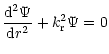 |
|
|
(4) |
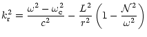
where the radial component of the local wave number,  ,
is given by
,
is given by
 |
|
|
(5) |
where c, is the radial distribution of sound speed,
 ,
defines a generalized critical frequency and
,
defines a generalized critical frequency and  ,
a generalized Brunt-Väisälä frequency,
that takes into account the geometrical terms and gravity
contribution for the local wave number,
which will be defined for each of the approximative motion equations.
is the
wave function, which is proportional to the Lagrangian perturbation
of pressure and will take a particular dependence, in agreement with
the approximation used.
,
a generalized Brunt-Väisälä frequency,
that takes into account the geometrical terms and gravity
contribution for the local wave number,
which will be defined for each of the approximative motion equations.
is the
wave function, which is proportional to the Lagrangian perturbation
of pressure and will take a particular dependence, in agreement with
the approximation used.
In the following analysis we will always consider this general case
given by Eq. (4),
unless we say explicitly the contrary.
2.1.1 The Planar approximation
In 1984, Deubner & Gough determined a linear second-order differential
equation in the standard form of the Eq. (4),
to describe the dynamics of adiabatic non-radial oscillations.
This equation of motion has been obtained by a procedure
analogous to the Lamb (1932) method. This approximation can be
made for waves with wavelength much smaller than the solar radius
and where the local effects of spherical geometry on the oscillatory
motion can be ignored. Additionally, the perturbations of the gravitational
potential have been ignored.
In this case, the wave function is given by,
 |
|
|
(6) |
where  ,
is the density and
,
is the density and  ,
is the Lagrangian
perturbation of pressure. In this case,
the local wave number, ,
is given by Eq. (5),
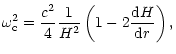
where the critical frequency,
,
is given by
,
is the Lagrangian
perturbation of pressure. In this case,
the local wave number, ,
is given by Eq. (5),
where the critical frequency,
,
is given by
 |
|
|
(7) |
where H, is the density scale height.
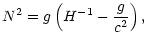
The generalized Brunt-Väisälä frequency, ,
is reduced to the classical Brunt-Väisälä frequency, N,
given by
 |
|
|
(8) |
where g, is the gravitational acceleration.
This model is particularly interesting because of the simplicity in the
interpretation of the characteristic frequencies of the equilibrium structure
that determine the cavities of propagative waves.
All the main properties of the local behavior of waves,
can be well defined in this approximation.
The equation of motion of stellar oscillations can be obtained by
reducing the fourth-order system of stellar oscillations to a second-order
differential equation, where the Eulerian perturbation of
the gravitational potential is neglected (Gough 1993). Cowling (1941)
showed the interest of this approximation, by
pointing out that it has a relatively minor effect on the modes,
with exception to the modes of low degree and low order.
Under the approximation proposed, i.e., neglecting
the contribution of the Eulerian pertubation of gravitational potential,
 ,
the initial fourth-order system of adiabatic stellar oscillations
is reduced to a second-order motion equation,
by the following transformation
,
the initial fourth-order system of adiabatic stellar oscillations
is reduced to a second-order motion equation,
by the following transformation
 |
|
|
(9) |
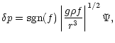
where sgn(f), is the sign of the discriminant f.
This discriminant, is given
by
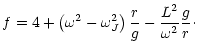 |
|
|
(10) |
 ,
is the square of the Jeans frequency,
that is equal to
,
is the square of the Jeans frequency,
that is equal to
 ,
where G is the gravitational
constant.
Using this transformation, the motion equation of
adiabatic nonradial stellar oscillations,
can be written in the form of Eq. (4).
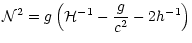
In that case, the generalized Brunt-Väisälä frequency,
,
is given by
,
where G is the gravitational
constant.
Using this transformation, the motion equation of
adiabatic nonradial stellar oscillations,
can be written in the form of Eq. (4).
In that case, the generalized Brunt-Väisälä frequency,
,
is given by
 |
|
|
(11) |
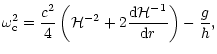
and the critical frequency,
,
is given by
 |
|
|
(12) |
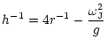
where
h is the scale height of g/r2 and
 is a generalized scale height.
The scale height h, is given by
is a generalized scale height.
The scale height h, is given by
 |
|
|
(13) |
and
,
is given by
 |
|
|
(14) |
where  ,
is the gravity scale height and Hf, is the
scale height of discriminant f.
A detailed discussion about these variables is presented in Gough (1993).
,
is the gravity scale height and Hf, is the
scale height of discriminant f.
A detailed discussion about these variables is presented in Gough (1993).
The difference between the generalization of the Brunt-Väisälä frequency,
and
the critical frequency,
relatively to these quantities
in the Deubner & Gough (1984) approach,
is due to the contribution of geometrical terms,
that can be important for the most penetrative modes in very
dense stars.
A more general solution to the initial system of stellar
oscillations can be obtained, which takes into
account a major contribution related with  .
This is called the first Post-Cowling approximation
(Gough 1993; Dziembowski & Gough, private comunication). Under this approximation the
Brunt-Väisälä frequency, ,
is given by
.
This is called the first Post-Cowling approximation
(Gough 1993; Dziembowski & Gough, private comunication). Under this approximation the
Brunt-Väisälä frequency, ,
is given by
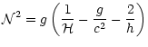 |
|
|
(15) |
and the critical frequency,
,
is given by
The total scale height ,
is given by
 |
|
|
(16) |
where the scale height
 takes into account
the contribution related with the
perturbation of the gravitational potential (Gough 1993;
Dziembowski & Gough, private comunication; Lopes 2001). The scale height
,
is given by
takes into account
the contribution related with the
perturbation of the gravitational potential (Gough 1993;
Dziembowski & Gough, private comunication; Lopes 2001). The scale height
,
is given by
 |
|
|
(17) |
The wave function, ,
can be determined as
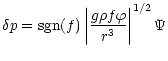 |
|
|
(18) |
where  ,
is a structure term related with the background state,
given by
,
is a structure term related with the background state,
given by
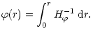 |
|
|
(19) |
These new expressions
for the characteristic frequencies come from a contribution related with the perturbation of
the gravitational potential which can be obtained from the linearized
Poisson equation. The magnitude of the effect relatively to the
classical Cowling approximation strongly depends on the density distribution
in the central region of the star.
2.2 Boundary conditions
The second-order motion equation together with two boundary
conditions, one at the centre and the other at the surface, forms
an eigen-value problem. We will present these boundary conditions
here, as they will be needed later.
The center is a regular singular point.
The regularity condition for the perturbation of
the Lagrangian variation of pressure, ,
is given by
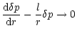 |
|
|
(20) |
as
 .
The outer boundary condition, is fixed in the atmosphere
and we consider that the inertia of the corona is so high
that ,
is given approximately by
.
The outer boundary condition, is fixed in the atmosphere
and we consider that the inertia of the corona is so high
that ,
is given approximately by
 |
|
|
(21) |
at r=R.
These simple conditions are sufficient to the discussion proposed
in this article.
These are the so-called "zero-boundary conditions'' (Unno et al. 1989).
The consideration of more realistic boundary
conditions does not modify significantly the method proposed to classify
modes in stars.
2.3 Propagation diagram
![\begin{figure}
\includegraphics[width=14cm]{2247f1.eps}
\end{figure}](/articles/aa/full/2001/27/aah2247/Timg69.gif) |
Figure 1:
Propagation diagram for a polytropic model with
index
 ,
adiabatic index ,
adiabatic index
 .
The curves correspond to a dimensionless circular frequency
relatively to the dimensionless radius.
These curves delimit the propagation region for modes of
degree .
The curves correspond to a dimensionless circular frequency
relatively to the dimensionless radius.
These curves delimit the propagation region for modes of
degree  :
a) The solid curves represent :
a) The solid curves represent
 computed in the Cowling approximation,
the dashed curves represent planar values of
,
and the dotted curves represent the Brünt-Väisäla frequency, N,
(increasing from the center to the surface) and the Lamb frequency,
computed in the Cowling approximation,
the dashed curves represent planar values of
,
and the dotted curves represent the Brünt-Väisäla frequency, N,
(increasing from the center to the surface) and the Lamb frequency,  ,
(decreasing from the center to the surface).
b) The solid curves represent
computed in
the first Post-Cowling approximation, and the dashed curve represents
in the Cowling approximation. ,
(decreasing from the center to the surface).
b) The solid curves represent
computed in
the first Post-Cowling approximation, and the dashed curve represents
in the Cowling approximation. |
| Open with DEXTER |
The direction and magnitude of the acoustic-gravity wave is determined by the
competition between the radial and tangential components of
the local wave number  ,
given by
,
given by
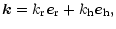 |
|
|
(22) |
where
 ,
,
 are unitary vectors in the
radial and horizontal directions and
are unitary vectors in the
radial and horizontal directions and
 (
(
 ), is the tangential component of the local wave number (Unno et al. 1989). The radial component of the local wave number,
is determined by the local properties of the equilibrium structure.
In this sense, it is possible to build a diagram for the radial component of the local
wave number, which defines the regions of propagative or evanescent behavior
of a given acoustic-gravity wave of frequency
and degree l.
This is the so-called propagation diagram.
Waves can propagate where the square of the vertical component of the local wave
is greater than zero, and are evanescent elsewhere.
This leads to two asymptotic limits, for the very high and for the very small
frequencies. In the case of very high frequencies,
), is the tangential component of the local wave number (Unno et al. 1989). The radial component of the local wave number,
is determined by the local properties of the equilibrium structure.
In this sense, it is possible to build a diagram for the radial component of the local
wave number, which defines the regions of propagative or evanescent behavior
of a given acoustic-gravity wave of frequency
and degree l.
This is the so-called propagation diagram.
Waves can propagate where the square of the vertical component of the local wave
is greater than zero, and are evanescent elsewhere.
This leads to two asymptotic limits, for the very high and for the very small
frequencies. In the case of very high frequencies,
 ,
the propagation
is predominantly in the radial direction. In the other case,
,
the propagation
is predominantly in the radial direction. In the other case,
 ,
then the propagation is predominantly in the horizontal direction.
This corresponds also to the spectral regions
where the restoring forces are dominated by gravity
(through the buoyancy) or pressure.
Because of that, it is convenient to write the local
wave number as a function of the critical frequencies
,
in which case ,
is given by
,
then the propagation is predominantly in the horizontal direction.
This corresponds also to the spectral regions
where the restoring forces are dominated by gravity
(through the buoyancy) or pressure.
Because of that, it is convenient to write the local
wave number as a function of the critical frequencies
,
in which case ,
is given by
 |
|
|
(23) |
where  is a discriminant, given by
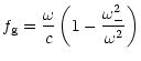 |
|
|
(24) |
and  is a discriminant, given by
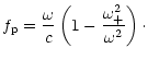 |
|
|
(25) |
The underscript g or p is fixed by the propagative regions that
are separated by
 or
or
 ,
respectively.
,
respectively.
It follows from Eq. (23) that
 ,
are real and
,
are real and
 and
and
 (acoustic or p-region, locally behaves like an acoustic type wave) or
 and
and
 (gravity or g-region, locally behaves like a gravity type wave). Here we will be mainly concerned with the case where
 and
and
 are both real.
In the case where
and
are complex conjugates
it is also possible to use the same analysis.
It will slightly complicate the algebra, but the physical conclusions remain the same.
are both real.
In the case where
and
are complex conjugates
it is also possible to use the same analysis.
It will slightly complicate the algebra, but the physical conclusions remain the same.
The critical frequencies
,
define the turning points of the
standard second-order differential equation,
previously presented, i.e.,
 .
In the more general case,
,
can be determined numerically. However
the critical frequencies
.
In the more general case,
,
can be determined numerically. However
the critical frequencies
 can be obtained,
by the relation,
can be obtained,
by the relation,
 |
|
|
(26) |
where, the Lamb frequency  ,
is given by
,
is given by
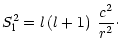 |
|
|
(27) |
In the case of Deubner & Gough (1984),
these expressions determine an explicit relation
of the critical frequencies as function
of the background structure and independent of the frequency
(see Sect. 2.1.1).
In Figs. 1 and 2 we present
the
computed critical frequencies,
,
for
the different approximations presented in the previous section,
in the case of polytropes of index
 and
and
 and adiabatic
index
.
A discussion about the
propagation of waves in polytropic equilibrium structure
with a different adiabatic index can be found in
Cowling (1941) and Scuflaire (1974).
The contribution related with the geometric
terms occuring in the variables
and
when
computed in the Cowling approximation is more important
for the more penetrative waves, i.e., waves with smaller degree,
as it is illustrated in Figs. 1a and 2a.
Similarly, the first Post-Cowling approximation,
seems worth considering in the case of stars with high density,
where the presence of the gravitational potential modifies
significantly the values of
in the central
region of the star
(cf. Figs. 1b and 2b).
and adiabatic
index
.
A discussion about the
propagation of waves in polytropic equilibrium structure
with a different adiabatic index can be found in
Cowling (1941) and Scuflaire (1974).
The contribution related with the geometric
terms occuring in the variables
and
when
computed in the Cowling approximation is more important
for the more penetrative waves, i.e., waves with smaller degree,
as it is illustrated in Figs. 1a and 2a.
Similarly, the first Post-Cowling approximation,
seems worth considering in the case of stars with high density,
where the presence of the gravitational potential modifies
significantly the values of
in the central
region of the star
(cf. Figs. 1b and 2b).
In the next section, using the differential Eq. (4) with the local
wave number given by Eq. (23), we will
write the standard equation of motion
in a convenient self-adjoint form, very appropriate for
the phase analysis that we will present below.
3 Phase analysis representation of the equation of motion
The phase method proposed here is based in a generalization
of a technique normally used
to study the solutions of a particular type of self-adjoint
second-order linear differential equation
with homogeneous boundary conditions, the so-called Sturm-Liouville problem.
This method consists in representing the eigenmodes in a convenient
Poincaré phase plane (in terms of polar coordinates),
normally used to study an autonomous system of differential equations.
In a first step,
we present two complementary self-adjoint forms of the
standard second-order differential equation
that describes the adiabatic nonradial oscillations of a
spherically symmetric star
(Eq. (4)).
Second, we present the phase analysis method to determine the eigenstates
of each of these self-adjoint differential equations,
where we introduce a classification scheme
that is build using the boundary conditions.
![\begin{figure}
\includegraphics[width=14cm]{2247f2.eps}
\end{figure}](/articles/aa/full/2001/27/aah2247/Timg98.gif) |
Figure 2:
Propagation diagram for Polytropic models of
index
,
 and adiabatic index
,
for modes of degree
and adiabatic index
,
for modes of degree  .
The representation adopted is the same as in previous Fig. 1. .
The representation adopted is the same as in previous Fig. 1. |
| Open with DEXTER |
3.1 Complementary self-adjoint differential equations
The
standard second-order differential equation of linear adiabatic stellar oscillations
(Eq. (4)), can be written into a pair of self-adjoint differential
equations. As we will discuss later, these equations should then be regarded as being
complementary to each other, for the study of the local properties,
related with the two driving mechanisms, pressure and gravity.
The transformation of the second-order differential equation into a
self-adjoint form will be done, taking into account the previous decomposition
related with the two propagation cavities for a given wave.
This is accomplished by the transformation,
 |
|
|
(28) |
where i=1,2 defines the two possible transformations,
related with two propagative regions.
We point out that, in the most general case, under these transformations
 does not conserve the location
and the number of zeros of the wave function .
We consider also that
does not conserve the location
and the number of zeros of the wave function .
We consider also that
 is a real function.
However, if the function
,
is conveniently chosen
(with no zeros in the whole interval considered) it
is possible to determine the location of the zeros for the
wave function ,
by the location of zeros of
.
Resulting in the following self-adjoint equation of motion,
is a real function.
However, if the function
,
is conveniently chosen
(with no zeros in the whole interval considered) it
is possible to determine the location of the zeros for the
wave function ,
by the location of zeros of
.
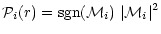
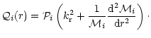
Resulting in the following self-adjoint equation of motion,
![$\displaystyle \frac{\rm d}{{\rm d}r}\left[{\cal P}_i (r) \frac{{\rm d}{\cal Y}_i}{{\rm d}r}\right] + {\cal Q}_i(r) {\cal
Y}_i=0,$](/articles/aa/full/2001/27/aah2247/img102.gif) |
|
|
(29) |
where
 ,
is given by
,
is given by
 |
|
|
(30) |
and
 ,
is given by
,
is given by
 |
|
|
(31) |
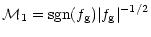
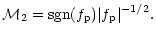
The function
,
can take two possible choices,
which will be in the mainframe of our analysis:
 |
|
|
(32) |
and
 |
|
|
(33) |
These two differential equations are equivalent to Eq. (4),
where
 is an invariant
of that family of equivalent differential equations.
The determination of
presented previously, has been done
under the consideration that
and
are real functions.
In the case they are complex conjugates then
is
defined as the real part of
and ,
respectively.
is an invariant
of that family of equivalent differential equations.
The determination of
presented previously, has been done
under the consideration that
and
are real functions.
In the case they are complex conjugates then
is
defined as the real part of
and ,
respectively.
These complementary equations will be very useful in the
analysis of the zeros of
the wave function, .
The location of the turning points will determine
what is the most convenient formulation to study the properties
of a given wave of frequency,
and degree, l, i.e., the formulation is chosen such that
is strictly positive
in the interval considered.
In fact, the localization of the singular points
depends on
and l, and they correspond to the zeros of
 or
or
 .
Choosing the convenient self-adjoint formulation for a given wave of
parameters
and l, the function
.
Choosing the convenient self-adjoint formulation for a given wave of
parameters
and l, the function
 is regular (
 )
in the interval
considered.
In this sense, in waves for which
)
in the interval
considered.
In this sense, in waves for which
 (
)
in all
the interval (acoustic type), the location of zeros of ,
corresponds to the location of zeros of
(
)
in all
the interval (acoustic type), the location of zeros of ,
corresponds to the location of zeros of
 ,
provided that
,
provided that
 does not have zeros on the interval considered.
Equation (29)
with i=1, is the convenient formulation to study the oscillatory motions.
Conversely, in waves for which
does not have zeros on the interval considered.
Equation (29)
with i=1, is the convenient formulation to study the oscillatory motions.
Conversely, in waves for which
 (
)
in
the interval considered (gravity type), the location of zeros of corresponds to the location of zeros of
(
)
in
the interval considered (gravity type), the location of zeros of corresponds to the location of zeros of
 .
Equation (29)
with i=2, is then the convenient formulation to study the oscillatory motions.
As we will discuss in Sect. 3.2, for some l and a mixing mode can appear and both descriptions will need to be used.
Under a correct choice of the self-adjoint form, the differential
Eq. (4)
for each of the propagative regions,
the number and the location of the zeros of ,
can all be determined from a convenient self-adjoint form, even in such case.
.
Equation (29)
with i=2, is then the convenient formulation to study the oscillatory motions.
As we will discuss in Sect. 3.2, for some l and a mixing mode can appear and both descriptions will need to be used.
Under a correct choice of the self-adjoint form, the differential
Eq. (4)
for each of the propagative regions,
the number and the location of the zeros of ,
can all be determined from a convenient self-adjoint form, even in such case.
In the following sections, when we are referring to a particular
formulation, we will use the underscript i on the
variables
,
and
,
with i=1 for the
acoustic description and i=2 for the gravity description.
This is a first step to the classification scheme that
will be defined like it was originally proposed by Cowling (1941),
taking into account
the two driving mechanisms, the gravity and the pressure.
3.2 Complementary phase equations
The phase analysis proposed here,
can be considered as a generalization of the method proposed by Eckart (1960),
Scuflaire (1974), Osaki (1975), Gabriel & Scuflaire (1979)
and Gough (1993) to discuss the classification scheme
of stellar oscillations.
The method proposed by these authors is
based on the algebraic counting of the number of nodes according to the
behaviour of p' relatively to
(or the other two wave functions).
In our case the classification scheme will be determined for a generic wave function that
can be related with
(for example), and the order of the mode will be determined
by the boundary conditions which can be, or not, reliable with the number of nodes
of this wave function.
The motion equation for linear adiabatic nonradial oscillations (Eq. (4))
can be transformed into
two self-adjoint differential equations (Eq. (29))
to determine the properties of the oscillations.
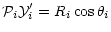
Using the phase transformation (with i=1, 2) for each of the self-adjoint forms
(see details about this phase analysis in Appendix A),
given by
 |
|
|
(34) |
and
 |
|
|
(35) |
where
 and
and
 are the amplitude and phase of the wave function
.
After some straightforward manipulation,
we obtain the following two first-order differential equations for the phase
(phase equations):
are the amplitude and phase of the wave function
.
After some straightforward manipulation,
we obtain the following two first-order differential equations for the phase
(phase equations):
 |
|
|
(36) |
and
 |
|
|
(37) |
where
 ,
is the real function given by
,
is the real function given by
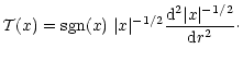 |
|
|
(38) |
The amplitudes in each case, are given by
![$\displaystyle R_1
=R_{1,{\rm o}}\exp{\left[
\frac{1}{2}
\int_{r_{\rm o}}^r
\lef...
...}-{\cal T}(f_{\rm g})
\right)
\sin{\left(2\theta_1\right)} \; {\rm d}r
\right]}$](/articles/aa/full/2001/27/aah2247/img126.gif) |
|
|
(39) |
and
![$\displaystyle R_2
=R_{2,{\rm o}}\exp{\left[
\frac{1}{2}
\int_{r_{\rm o}}^r
\lef...
...}-{\cal T}(f_{\rm p})
\right)
\sin{\left(2\theta_2\right)} \; {\rm d}r
\right]}$](/articles/aa/full/2001/27/aah2247/img127.gif) |
|
|
(40) |
where
 is the initial amplitude.
At this level, it is important to point out that Eqs. (36)
and (37) are two different phase representations of the same physical
system described by Eq. (4), written in a way that it avoids singular points
for a given wave of degree l and frequency ,
in a given region.
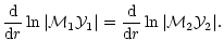
It is possible to determine a relation between
the two phases, which is obtained by imposing a matching of the logarithmic derivatives
of
(Eq. (28)) between both descriptions. This is given by
 |
|
|
(41) |
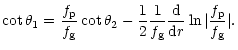
Using Eqs. (32) and (33) with the phase relation A.5,
we obtain the following relation between phase  and
and  :
:
 |
|
|
(42) |
This relation can be used to
determine the phase
(of the acoustic description)
knowing the phase
(of the gravity description).
We observe that when we want to convert
into
(go from the gravity description to the
acoustic description),
the point where
is singular,
so that
 ,
and consequently
,
and consequently
 .
Finally, we note that Eq. (42) is undefined
in the radius where
.
However this situation never happens within this transformation.
.
Finally, we note that Eq. (42) is undefined
in the radius where
.
However this situation never happens within this transformation.
In short, the propagation of a wave of degree l and frequency
can be explicitly determined for any of the three types of waves
(which can be defined from the propagation diagrams)
using the appropriate phase equation.
For the pure acoustic type waves, the phase can be determined from
Eq. (36) (acoustic description) because no singular points occur
inside.
For the pure gravity type waves,
the phase can be determined by Eq. (37) (gravity description).
Furthermore, for mixed type waves which correspond to a mode
that propagates in two different regions,
Eq. (36) can be used
to determine the phase propagation on the gravity region
and Eq. (37) to determine the phase
propagation on the acoustic region.
The matching condition is made in the region where both descriptions,
are accepted (without singular points). A possible choise is a point  ,
where
,
where
 and
and
 ,
in that case from Eq. (42)
we obtain
,
in that case from Eq. (42)
we obtain
 .
To make the matching we integrate each of
the equations from each side of the interval and match them in the point
.
To make the matching we integrate each of
the equations from each side of the interval and match them in the point  ,
where both solutions are valid.
,
where both solutions are valid.
3.3 Boundary conditions
The stellar oscillation eigenmodes can be determined by using one of
the phase equations (Eqs. (36) or (37)),
with a convenient set of boundary conditions at the endpoints, the centre and
the surface. The phase equations are equivalent one another and the choice of
which discription to use is matter of the tast of the author as well the type
of singularities that can be enconter. Indeed, a certain phase equation with the
respective boundary conditions at the center and the surface, constitutes an eigen-value
problem. In the following, we will indicate how it is possible to determine the boundary
conditions for each representation.
The phase at the endpoints is determined by using one of two procedures.
One consists in transforming the boundary conditions
of the eigenfunction
or (see Sect. 2.2) into an equivalent endpoint condition
for the phase function  of the phase associated system, related with
the differential Eq. (29).
Independent of the approximation made on the
determination of the local wavenumber, defined on
the equation of motion (see Sect. 2),
it is possible to determine the phase at the endpoints
from the Lagrangian perturbation of pressure and the Eq. (A.5).
In the Appendix B, we present the determination of the boundary condition
in the case of the planar approximation (Deubner & Gough 1984).
of the phase associated system, related with
the differential Eq. (29).
Independent of the approximation made on the
determination of the local wavenumber, defined on
the equation of motion (see Sect. 2),
it is possible to determine the phase at the endpoints
from the Lagrangian perturbation of pressure and the Eq. (A.5).
In the Appendix B, we present the determination of the boundary condition
in the case of the planar approximation (Deubner & Gough 1984).
An alternatively method consists in determining the phase at the endpoints
by imposing the regularity of the phase function .
A detailed analysis of the phase Eqs. (36) and (37),
indicates that these ones are singular at the endpoints, r=0 (for all stars)
and r=R (only for polytropes).
This implies that the boundary conditions must be applied
such that the singular solution at each of the endpoints is eliminated.
This is obtained by expanding the solution, ,
as a power series of r, relatively to the critical endpoint.
It is necessary also to expand the equilibrium quantities
around the endpoints, r=0 and r=R.
It is worth to notice that for each description it is possible to
study the properties of the gravity waves, as well as of the acoustic waves, even if
it is more convenient to use a gravity description to study the eigenstates
of gravity perturbations and similarly the acoustic description to study the eigenstates
of acoustic perturbations. In that case for each description, we will refered to the perturbation
as characterized by the main contributer for the restoring force
that is present in a certain region inside the star. In this context, we will refered
to an acoustic behaviour or the gravity behaviour,
as it is the gravity or the pressure the main contributer for the restoring force.
The mixed modes can be treated as a combination of these two "asymptotic'' cases
(as discussed in the previous section),
as an acoustic type mode or gravity type mode for each of the region where one
of these character prevails.
In particular, the inner and outer boundary conditions
for mixed modes are determined based in which is the dominant wave
character near the center or
near the surface of the star.
The inner boundary condition near the center is obtained by imposing that the solution to the phase
equation is regular, i.e.
has a finite value. Now, we will illustrate that by considering
the case corresponding to the acoustic description, i.e., we are interested in determine the
solution,
as given by Eq. (36). Furthermore, we will starting by
considering a wave that has an acoustic behaviour near the stellar center,
it follows that
must be a regular function at the center, as the phase has a finite value.
We notice that the first-member of Eq. (36) is singular, consequently, the
finite value of
 is obtained by choosing all the multi-value solutions,
such as
where n is a positive or a negative integer
(or in an equivalent form
is obtained by choosing all the multi-value solutions,
such as
where n is a positive or a negative integer
(or in an equivalent form
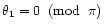 ;
see also Appendix B). Similary in the
case of the gravity description (Eq. (36)),
a wave with a gravity behaviour at the center has a regular solution
if
;
see also Appendix B). Similary in the
case of the gravity description (Eq. (36)),
a wave with a gravity behaviour at the center has a regular solution
if
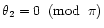 .
It follows that the same boundary conditions
can be presented in both descriptions, given that
.
It follows that the same boundary conditions
can be presented in both descriptions, given that
 .
This relation between phases is illustrated in the next section.
In resume, the boundary condition for the center require
that
.
This relation between phases is illustrated in the next section.
In resume, the boundary condition for the center require
that
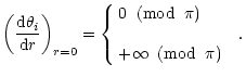 |
|
|
(43) |
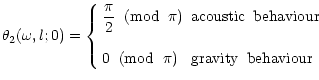
Alternativelly, from the
phase Eqs. (36) and (37)
it follows in the case of the acoustic description,
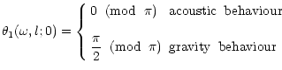 |
|
|
(44) |
for modes with acoustic and gravity behaviour near the centre
of the star, and
in the case of the gravity description,
 |
|
|
(45) |
for modes with acoustic or gravity behaviour.
The outer boundary condition, can be obtained also by a series expansion
around the endpoint r=R.
In the case of polytropic equilibrium structures,
because the sound speed is zero at r=R, the
phase Eqs. (36) and (37) can be singular. It follows that
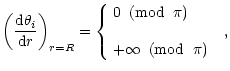 |
|
|
(46) |
then we obtain the following type of conditions for the surface,
 |
|
|
(47) |
and
 |
|
|
(48) |
An approximative solution can be obtain by using the results of Appendix B.
We start bu notice, that the sound speed vanish at the surface, consequently, we have
 and
and
 .
In case of acoustic description if we consider the asymptotic limit,
.
In case of acoustic description if we consider the asymptotic limit,
 ,
then
,
then
 ,
or
,
or
 (mod
(mod  )
and in the case of gravity description if we consider the asymptotic limit
)
and in the case of gravity description if we consider the asymptotic limit
 then
then
 or
or
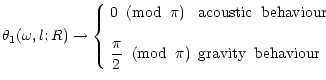
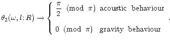
 (mod ). Consequently,
following a similar procedure to study the solution in the center
of the star, we can obtain the expression for the two type of waves in both descriptions.
It follows,
(mod ). Consequently,
following a similar procedure to study the solution in the center
of the star, we can obtain the expression for the two type of waves in both descriptions.
It follows,
 |
|
|
(49) |
and
 |
|
|
(50) |
In real stars this outer boundary condition can be slightly different,
but the main conclusion remains the same.
We observe that with these boundary conditions for the
inner endpoint, in both descriptions both solutions are regular
because the amplitude and the phase have finite values for r=0.
3.4 Simplified phase equations
Ledoux & Walraven (1958) have derived a particular solution,
which presents two asymptotic limits for very high
and very small eigenfrequencies. In this case the system of stellar oscillations under the
Cowling approximation tends toward a Sturm-Liouville type solution.
Here, an analogous situation takes place, when the term with the form
,
in Eqs. (36) and (37) can be neglected.
This is a good approximation in most of the stellar interior,
because this term remains small compared with
the other terms almost everywhere, except near the turning points
(where
or
becomes 0)
and the stellar surface.
In that case,
the nodes of
(or
)
correspond
to extremes of
(or
).
The phase equations take the simple form:
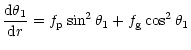 |
|
|
(51) |
and
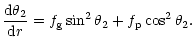 |
|
|
(52) |
In that case the phase between the two prescriptions has
the very simple relation,
 .
It is also important to remark that, in a given representation
when a solution at the initial endpoint is singular,
it is regular at the other phase representation.
This lead us to use a convenient phase repesentation
to avoid this singular behaviour, which is the origin of
the acoustic and gravity description presented in the last
section.
.
It is also important to remark that, in a given representation
when a solution at the initial endpoint is singular,
it is regular at the other phase representation.
This lead us to use a convenient phase repesentation
to avoid this singular behaviour, which is the origin of
the acoustic and gravity description presented in the last
section.
It is important to stress that this is a very good representation for
the phase equations and from that we can say that the difference between the
acoustic and gravity waves presents a shift of  .
In this case, it is very clear the fact that both phase equations are strictly
equivalent.
.
In this case, it is very clear the fact that both phase equations are strictly
equivalent.
For a given l, if  is large this suggests the existence of
a spectrum of indefinitely increasing eigenvalues, corresponding to the eigensolution denoted by
acoustic modes or p-modes.
Conversely, for
very small, this tends to define a Sturm-Liouville problem with
the parameter
is large this suggests the existence of
a spectrum of indefinitely increasing eigenvalues, corresponding to the eigensolution denoted by
acoustic modes or p-modes.
Conversely, for
very small, this tends to define a Sturm-Liouville problem with
the parameter
 ,
which
corresponds to the eigensolutions denoted by gravity modes or g-modes.
,
which
corresponds to the eigensolutions denoted by gravity modes or g-modes.
4 Propagation of acoustic-gravity waves
The stellar oscillations are now described by one or another
phase equations (Eqs. (36) and (37)).
These phase equations with the
respective boundary conditions 44 and 47
or 45 and 48 form a boundary value problem
with
as an eigenvalue.
In this section we start by determining numerically the eigenfrequencies that are solutions
of the eigenvalue problem presented. By the following, we will present a classification
scheme base in the result obtained.
Let's start by observing that the phase function
 (mod ), has the same
number of zeros at the same location as the wave function ,
provided that
the transformations
are made as was indicated previously.
However, the number and location of the zeros of the wave function, ,
(obtained from the equation of motion, Sect. 2), are the same
as ,
only for pure acoustic or gravity modes, due to the fact that the discriminant fas given by Eq. (10)
is strictly positive or negative in all the star.
In the case of mixed modes, another zero occurs for the wave function,
,
at the radius of the star where f=0.
(mod ), has the same
number of zeros at the same location as the wave function ,
provided that
the transformations
are made as was indicated previously.
However, the number and location of the zeros of the wave function, ,
(obtained from the equation of motion, Sect. 2), are the same
as ,
only for pure acoustic or gravity modes, due to the fact that the discriminant fas given by Eq. (10)
is strictly positive or negative in all the star.
In the case of mixed modes, another zero occurs for the wave function,
,
at the radius of the star where f=0.
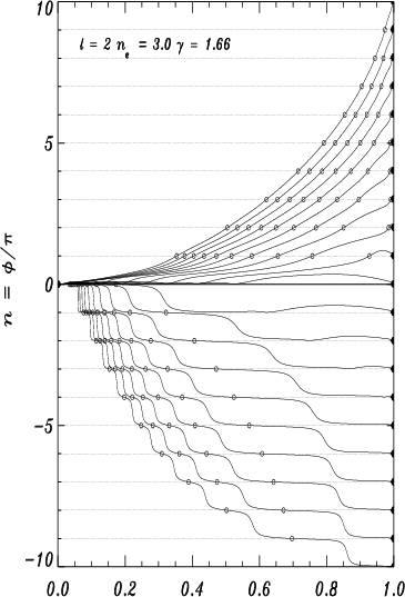
The main properties of the stellar oscillations, can be well defined
in a linear phase diagram (see Fig. 4) that determines the
phase dependence of a given eigenmode with the radius, for a given equilibrium structure.
The construction of the linear phase diagram is made by introduction of
an effective phase,
 .
This effective phase for each eigenmode, of
an eigenvalue
and degree l, is given by
.
This effective phase for each eigenmode, of
an eigenvalue
and degree l, is given by
 |
|
|
(53) |
where ,
is the phase function.
The computation of the linear phase diagram is made using the phase
Eq. (36) in the case of acoustic modes, and
the Eq. (37), with
 ,
in the case of gravity modes. In that case the linear phase diagram
for acoustic and gravity modes is constructed based in the phase
.
This is justified by the simple relation between
acoustic and gravity description when the function
,
in the case of gravity modes. In that case the linear phase diagram
for acoustic and gravity modes is constructed based in the phase
.
This is justified by the simple relation between
acoustic and gravity description when the function  is neglected
in the phase equation.
We remember that an eigenmode is the product of an amplitude function
by a phase function, and the main properties of the eigenmode
can be discussed using the phase equation.
is neglected
in the phase equation.
We remember that an eigenmode is the product of an amplitude function
by a phase function, and the main properties of the eigenmode
can be discussed using the phase equation.
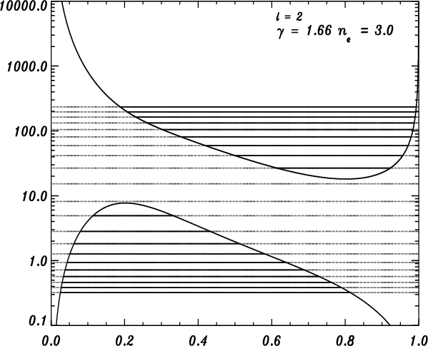
 |
Figure 3:
Propagation diagram
for a polytropic model with index
,
adiabatic index
and modes of degree l=2. The solid curves
represent the critical frequencies
 ,
delimiting the two propagation regions of the stellar oscillations
as it is obtained from the first Cowling approximation motion equation
(see text). The eigenstates
corresponding to the eigenmodes with dimensionless square of the
circular frequency, :
234, 196, 163, 132.4, 104.8, 80.55, 59.42, 41.47,
26.72, 15.26, 8.175, 4.915, 2.828, 1.822, 1.270,
0.9360, 0.7188. ,
delimiting the two propagation regions of the stellar oscillations
as it is obtained from the first Cowling approximation motion equation
(see text). The eigenstates
corresponding to the eigenmodes with dimensionless square of the
circular frequency, :
234, 196, 163, 132.4, 104.8, 80.55, 59.42, 41.47,
26.72, 15.26, 8.175, 4.915, 2.828, 1.822, 1.270,
0.9360, 0.7188. |
| Open with DEXTER |
The nonradial oscillations of a star
can be interpreted as a superposition of stationary waves
generated by the competition between the pressure and the gravity.
These two driving mechanisms, define the two
propagation regions illustrated in the Fig. 3
for a polytropic equilibrium structure of index
.
An eigenstate, can be interpreted heuristically as being
the result of the competition between these two propagative regions,
as it is determined by the phase Eq. (36)
(or Eq. (37)).
The eigenstates corresponding to the acoustic waves of high frequency,
can be determined neglecting the contribution of the
gravity propagation region (which corresponds to neglecting
the second term of Eq. (36),
which case is similar to the Sturm-Liouville problem.
In this case, the modes form a well-ordered sequence,
starting from a given fundamental state.
Conversely, the eigenstates of gravity waves of very low frequency,
can be determined by neglecting the contribution of the acoustic propagation.
A particular state occurs in the star, even in a very simple
equilibrium structure, caused by the fact
that both propagative regions contribute in the same order of magnitude
for this standing wave. This corresponds to the f-mode. Furthermore,
this eigenmode presents a mixed nature and propagates mainly or uniquely
in the evanescent region of the star.
Cowling (1941) was the first to point out
the fundamental difference of nature of the f-mode,
relatively to the p-modes and g-modes.
The f-mode corresponds to the fundamental oscillation of the system for
which no nodes occur on the wavefunction.
Furthermore, for stars where mixing of modes can occur, this
f-mode, as it is defined here, cannot exist.
It is possible to prove that
the modes form a well-ordered sequence when the star is
simple,
given that two different eigenmodes never cross.
However, this can be guaranteed only for modes that propagate locally as an
acoustic type wave or
gravity type wave. The evanescent type mode f is the only exception.
The fact that the phase of two eigenmodes never crosses, is reliable on the topological
properties of the propagation diagram
(see Figs. 1, 2 and 3)
and the properties
of the phase equations. For two waves with frequencies,  and
and  ,
such as
,
such as
 ,
the propagative characteristics
are fixed differently for an acoustic-gravity wave,
in function of the type of propagation.
For a wave that propagates acoustically,
the higher frequency presents always a larger propagative
region.
Conversely, for a wave that propagates by gravity type,
the higher frequency presents always a smaller propagative
region. Furthermore, on the propagative region, we have that
,
the propagative characteristics
are fixed differently for an acoustic-gravity wave,
in function of the type of propagation.
For a wave that propagates acoustically,
the higher frequency presents always a larger propagative
region.
Conversely, for a wave that propagates by gravity type,
the higher frequency presents always a smaller propagative
region. Furthermore, on the propagative region, we have that
 ,
for two waves that propagate acoustically,
and
,
for two waves that propagate acoustically,
and
 ,
on the other cases.
Using the phase equations corresponding
to each one of these descriptions,
we have that
,
on the other cases.
Using the phase equations corresponding
to each one of these descriptions,
we have that
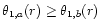 for acoustic type propagation
and
for acoustic type propagation
and
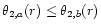 for gravity type propagation, for each point inside the star.
This determines that two eigenmodes can never cross each other,
if they are acoustic waves, gravity waves or mixed waves.
for gravity type propagation, for each point inside the star.
This determines that two eigenmodes can never cross each other,
if they are acoustic waves, gravity waves or mixed waves.
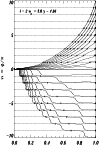 |
Figure 4:
Linear phase diagram for a polytropic
equilibrium model of index,
,
and adiabatic index
.
The curves represent the phase function
 of
eigenmodes of frequency
and degree l=2.
The thin-dashed straight lines represent the number -cycle
that a phase function has developed from the internal endpoint
r=0, until the external endpoint r=R. The inner boundary
condition at r=0 and the outer boundary condition at r=R for
the different cycles of
are represented by a black dot. In
the propagative regions where the eigenmodes behave like an
acoustic wave the phase increases (clockwise direction) and in
propagative regions where the eigenmodes behave like a gravity
wave the phase decreases (anticlockwise direction). The phase
function,
of
eigenmodes of frequency
and degree l=2.
The thin-dashed straight lines represent the number -cycle
that a phase function has developed from the internal endpoint
r=0, until the external endpoint r=R. The inner boundary
condition at r=0 and the outer boundary condition at r=R for
the different cycles of
are represented by a black dot. In
the propagative regions where the eigenmodes behave like an
acoustic wave the phase increases (clockwise direction) and in
propagative regions where the eigenmodes behave like a gravity
wave the phase decreases (anticlockwise direction). The phase
function,  is calculated for a given eigenstate, from the
higher to the lower eigenfrequencies. The radial order number,
is calculated for a given eigenstate, from the
higher to the lower eigenfrequencies. The radial order number,
 ,
takes values from 10 to -10 (see text). ,
takes values from 10 to -10 (see text). |
| Open with DEXTER |
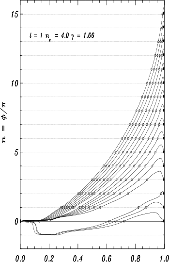
In Figs. 3 and 4
we represent the propagation
diagram and the linear phase diagram for the eigenmodes of degree l,
for a polytropic equilibrium structure of index
and adiabatic index
.
The phase function of acoustic waves and gravity waves,
present important propagative topological differences between them.
However, for the very low frequency acoustic waves and high frequency
gravity waves, the propagation is similar to a f-mode.
The main asymptotic properties can be illustrated in
the planar approximation (see Appendix B).
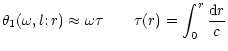
In the case of acoustic modes, corresponding to the higher frequencies
(
 ), the
phase Eq. (36) is dominated by the term
), the
phase Eq. (36) is dominated by the term  ,
through the discriminant
and .
Then the phase, ,
is given approximatively by
,
through the discriminant
and .
Then the phase, ,
is given approximatively by
 |
|
|
(54) |
where  ,
is the so-called acoustic radius.
However, the phase stays practically constant on the evanescent regions.
,
is the so-called acoustic radius.
However, the phase stays practically constant on the evanescent regions.
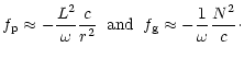
Alternatively, the gravity modes
are given by Eq. (37), corresponding to the smaller frequencies
(
),
the discriminants
and
can be approximated by
 |
|
|
(55) |
In that case, we have a competition between these two terms,
which give the waviness pattern, characteristic of the phase function of gravity waves.
It is possible to demonstrate that the asymptotic leading term,
in this case leads to

 .
.
In the example presented above, mixing of modes does not occur
(no overlap of the propagative region),
but if this happens, the phase function presents
a similar behaviour to the acoustic and gravity modes
for each one of the respective propagation regions (see Fig. 2b).
5 Classification of stellar oscillations
To discuss the differences between the new
classification scheme proposed in this work relatively
to the classification schemes normally used, we present in the following the
original classification proposed by Cowling (1941) and the generalization
of that one made by Eckart (1960), Scuflaire (1974) and Osaki (1975).
The first classification scheme to label
the eigenmodes of oscillations was introduced by T. Cowling (1941).
This is valid
provided that the reduction of the fourth-order system of
nonradial adiabatic stellar oscillations to a second-order
system is obtained under the hypothesis that the Eulerian perturbation of the
gravitational field
can be ignored. This scheme provides a good qualitative description of
higher-order modes for l=0 and l=1 and for all the modes with
 .
.
Formally, the frequency is unbounded below (except when l=0),
and also unbounded above.
Therefore, it is not immediately obvious where to choose the origin
of n. It is possible to choose n such that as
 for a fixed l, |n|-1 is the number of zeros in the eigenfunction,
when
and |n| is the number of zeros in the eigenfunction,
when l = 0.
For spherically symmetrical modes (l=0),
the lowest-frequency mode (fundamental mode) is labeled n=1.
In simple stellar models, modes with n >0 and n <0 have the
characteristics of acoustic and internal gravity waves;
they were designated p-modes and g-modes by Cowling (1940).
Modes with n=0, are fundamental g-modes or f-mode, and
have the property that when
for a fixed l, |n|-1 is the number of zeros in the eigenfunction,
when
and |n| is the number of zeros in the eigenfunction,
when l = 0.
For spherically symmetrical modes (l=0),
the lowest-frequency mode (fundamental mode) is labeled n=1.
In simple stellar models, modes with n >0 and n <0 have the
characteristics of acoustic and internal gravity waves;
they were designated p-modes and g-modes by Cowling (1940).
Modes with n=0, are fundamental g-modes or f-mode, and
have the property that when  ,
they have no zeros in the
eigenfunction.
Under these considerations, the modes of a star can be classified as
p-modes for n>0 and g-modes for n<0, and a (unique) f-mode
for n=0. Then both g and p sequences start from n=1.
The fundamental l=0 mode, was labeled with n=1.
,
they have no zeros in the
eigenfunction.
Under these considerations, the modes of a star can be classified as
p-modes for n>0 and g-modes for n<0, and a (unique) f-mode
for n=0. Then both g and p sequences start from n=1.
The fundamental l=0 mode, was labeled with n=1.
The Cowling classification scheme has been generalized by Eckart (1960),
by taking into account the tunnel effect that can take place when
the competition between the two restoring forces pressure and gravity
is of the same order.
Eckart (1960) discusses how the phase differences between vertical
displacement and pressure fluctuation decreases with height for acoustic modes
and increase for g-modes, so that order n can be computed by first
assigning a signal to each zero in the eigenfunction according to the
direction of variation of the phase difference, and then counting the zeros
algebraically.
Scuflaire (1974) and Osaki (1975) presented the same criterion to classify stellar
oscillations.
Scuflaire (1974) has demonstrated that, for relatively condensed polytropic modes
 (in case of modes of degree l=2) and
,
the mixing of modes (in the Cowling approximation) occurs.
This classification scheme, has been found to work well in most stars for oscillations with
,
when the Cowling approximation is not considered.
The problem remains for l=1.
Another classification scheme was proposed by
Shibahashi & Osaki (1976),
based on the properties of the wave on the main trapping region.
(in case of modes of degree l=2) and
,
the mixing of modes (in the Cowling approximation) occurs.
This classification scheme, has been found to work well in most stars for oscillations with
,
when the Cowling approximation is not considered.
The problem remains for l=1.
Another classification scheme was proposed by
Shibahashi & Osaki (1976),
based on the properties of the wave on the main trapping region.
However, none of these classification schemes
is sufficiently general. This is due to two main reasons.
One, is the fact that the classification scheme is dependent on the eigenfunction
used to determine the order n of the mode, which in the most general case does not
necessarily have the same number of zeros of other eigenfunctions
choosen also to classify the modes of some physical system (Cox 1980).
This means that the classification scheme depends on the properties
of the wave function choosen to define the system,
as it has been illustrated by different authors (Cox 1980 and references there).
The classification scheme does not work for modes with  .
Even if we consider that this hypothesis is acceptable,
there is a second problem which remains.
It is the fact that all the classification scheme
has been done under the Cowling approximation, and the full problem
is just an extension of this case.
.
Even if we consider that this hypothesis is acceptable,
there is a second problem which remains.
It is the fact that all the classification scheme
has been done under the Cowling approximation, and the full problem
is just an extension of this case.
The resonant cavities are clearly defined for all modes of any order,
and not only for modes of high-order and very high degree, as
is normally done in the most classical scheme classifications.
We start by pointing out,
that the phase functions
 ,
only depend on the
structure of the equation of motion, i.e. on the topology of the propagation
diagram.
,
only depend on the
structure of the equation of motion, i.e. on the topology of the propagation
diagram.
The oscillation corresponding to an eigenstate, can be defined
in terms of the boundary conditions, where
is a parameter.
In this sense, an eigenstate occurs when
the difference of phase between the initial phase at r=0and the final phase
at r=R, are a multiple of .
This introduces a natural scheme classification for the eigenmodes,
which determines the order number of the mode, n,
as the integer associated to the total number of
-cycles that the phase function
has developed from the
inner endpoint where the inner boundary condition is fixed until the outer
endpoint where the outer
boundary condition is fixed (see Sect. 4).
The determination of the eigenvalue equation,
similar to the Bohr-Sommerfeld quantization rule, is done in one
particular description given that, as we mentioned previously,
both descriptions are equivalent.
An eigenstate corresponds to the following
condition for each of the wave types:
 |
|
|
(56) |
where
 is the difference between the outer boundary
condition fixed for r=R, given by
is the difference between the outer boundary
condition fixed for r=R, given by
 and the inner boundary condition given by
 .
In our case it is given by the expression 47
(or 48).
n, is a negative or positive integer, starting from 0.
The well-ordered sequence
of eigenfrequencies,
corresponding to the ordering of the integer n, from
.
In our case it is given by the expression 47
(or 48).
n, is a negative or positive integer, starting from 0.
The well-ordered sequence
of eigenfrequencies,
corresponding to the ordering of the integer n, from
 to
to  ,
is guaranteed by the properties of the phase
function discussed in the last section.
The only exception is the unique f-mode.
It will be positive, if
,
is guaranteed by the properties of the phase
function discussed in the last section.
The only exception is the unique f-mode.
It will be positive, if
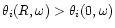 and it will be negative in the opposite case.
The negative integer is reserved for the gravity modes,
and the positive integer for the acoustic modes.
However in the case of mixed modes the sign of n,
determines the dominant character of the propagation mode.
This classification scheme is general and
is fixed by the boundary conditions, and does not depend on the
turning points of the modes, or even on the algebraic counting
of the number of nodes of
the eigenfunction (i.e. the number of
cycles, that the
phase function has developed from the internal endpoint, until
the external endpoint).
and it will be negative in the opposite case.
The negative integer is reserved for the gravity modes,
and the positive integer for the acoustic modes.
However in the case of mixed modes the sign of n,
determines the dominant character of the propagation mode.
This classification scheme is general and
is fixed by the boundary conditions, and does not depend on the
turning points of the modes, or even on the algebraic counting
of the number of nodes of
the eigenfunction (i.e. the number of
cycles, that the
phase function has developed from the internal endpoint, until
the external endpoint).
The more condensed polytropes
(see Fig. 2b)
cannot have the f-mode.
However, the degeneracy of the eigenstates of low
order modes can occur more frequently due to the overlap of the two propagative regions.
In Figs. 3 and 4 we present
the propagation diagram and the linear phase diagram of a polytope
of index
.
The high values of |n| correspond to
pure acoustic waves for positive values of n and
pure gravity waves for negative values of n.
This occurs because these waves present only one propagative region and a well
behaved phase function in each case.
In that case, the main properties are conserved for modes of low radial
order.
However, in the case of condensed polytropes such as polytropes of index
,
for the lower radial order modes,
the wave function presents a mixed character
which is determined by each of the two propagative regions.
In this case the eigenstate can occur by two possible ways:
or the eigenstate is mainly determined in only one of the
propagative regions, or is fixed by both propagative regions when the evanescent region
between them is small compared with the wavelength of the wave, i.e., tunnel effect.
It will be the particular topological nature of the propagation diagram
that will determine the different eigenstates.
In such cases
the previous classification fails for modes
of low degree, particularly those with l=1, in highly condensed
stellar models. In the scheme presented, the dipole modes have a perfect
ordering, even for the lowest orders,
such as  .
This is evident for modes
of a polytrope of index
with
.
This is evident for modes
of a polytrope of index
with  ,
l=1 (see Fig. 5).
The lower-order modes have phase paths quite different from those of
the higher-order modes, because the perturbation to the
gravitational potential in the central region can change the
character, in regions where the mode behaves like a gravity wave.
We believe that this is the reason why previous classification
schemes do not work. This behaviour
is likely to occur in real stars (Lopes 2000).
,
l=1 (see Fig. 5).
The lower-order modes have phase paths quite different from those of
the higher-order modes, because the perturbation to the
gravitational potential in the central region can change the
character, in regions where the mode behaves like a gravity wave.
We believe that this is the reason why previous classification
schemes do not work. This behaviour
is likely to occur in real stars (Lopes 2000).
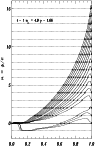 |
Figure 5:
Linear phase diagram of modes of degree l=1,
for a polytropic model of index,
and adiabatic index
.
The representation adopted is the same of the
previous figure. |
| Open with DEXTER |
It is convenient, also to point out the agreement between
this method and the classical method proposed by Cowling (1941) and others,
for the higher order modes of simple stars
(see Fig. 4).
For example, for a polytrope of
the eigenstate of order n=10,
corresponds to an acoustic mode, for which the phase function, presents 11 nodes
(i.e. -cycles of the phase function)
and is classified with n=10 in the classical scheme.
A gravity wave, of order n=6presents 7 nodes and is classified with n=6 in the classical scheme.
Finally, we observe that only in the case of a Sturm-Liouville eigenvalue type problem,
it is guaranteed that the eigenfunction associated to some eigenvalues,
has exactly n zeros (Cowling 1941).
It is just in eigenvalue problems similar to that one that it is possible
to use the counting of the zeros of the eigenfunction to label the order of the eigenstate.
Moreover, the algebraic counting of zeros of the eigenfunction on the
gravity region or the acoustic region can also be used
to label the states of the system (Scuflaire 1974).
This is on the basis of the usual classification schemes,
and it is one of the reasons why they do not work.
6 Summary and conclusion
It has been known since the first classification scheme
proposed by Cowling (1941) and later developed
by Scuflaire (1974) and Osaki (1975), that the
classification of modes for relatively evolved stars is ambiguous.
This problem in the classification
arises from the fact that the complete fourth-order system
of stellar nonradial adiabatic oscillations has been obtained
by a simple extension of the classification scheme
proposed by Cowling (1941) for a second-order system,
obtained by neglecting the Eulerian perturbation of the gravitational
potential in the full problem. Furthermore, any classification scheme depends
on
the wave function choosen to determine the eigenstates of the oscillatory system
and on its number of zeros.
In this work, we have addressed the problem determining a unique
classification scheme for the equation of motion,
independent of the eigenfunction used to characterize
the oscillatory motion and its number of zeros.
The principle consists in determining two self-adjoint forms
of the equation of motion, build by using the
propagation diagram which
is associated with the different types of stellar perturbations,
that overcome from the restoring force due to the
competition between the pressure and the gravity.
All the properties of the eigenmodes depend only on the
topological properties of the propagation diagram.
For each of the self-adjoint forms of the equation of motion,
a phase representation of
the eigenmode is made which consists in describing the oscillatory
motion of adiabatic oscillations by a system of two
first-order nonlinear differential equations for the phase and the
amplitude. The equations are coupled only in the amplitude equation,
leaving a single phase equation to determine the eigenfrequencies.
A convenient phase representation is determined for each
type of propagation, corresponding to each case, whether is
the pressure or the gravity that dominates in the restoring force.
This competition between the pressure and gravity,
can generate 3 types of waves for which the local properties
can be defined on a propagation diagram together
with the respective linear phase diagram,
for which the linear phase properties are distinct from each other.
Furthermore, the linear phase diagram proposed, constitutes a powerful
method to determine an unique radial order number n.
Similarly to the classical methods,
the sign of order number n determines the dominant
nature of the wave.
A possible atempt to classified the eigenvalues of the
linear adiabatic nonradial oscillation system (of the fourth-order problem of nonradial
adiabatic oscillations), is to determine the radial order
n of the eigenmode by using the phase equations Eqs. (36) and
(37) with the
respective boundary conditions given by Eqs. (44) and (47)
or (45) and (48). In that way,
this technique can be used to constrain the linear phase diagram,
which can determine the unique radial order number n. However, it is
expected that this technique will not work in all the cases, once
the second-order system have been obtained by an approximative method.
A more extensive study must be made to identify those
cases that this porcedure can be applied.
Finally, the classical scheme proposed by
Scuflaire (1974) and Osaki (1975) corresponds to a particular case of
this general scheme, for which the order number
n is equal to the algebraic counting of the number of modes in the different
propagative regions, with a positive sign for modes in the acoustic propagative
region and a negative sign for modes in the gravity propagative region.
Acknowledgements
Ilídio Lopes thanks Douglas Gough for stimulating discussions
on the oscillatory properties of acoustic waves and stellar
modelling. He also acknowledges support of a grant from the
Particle Physics and Astronomy Research Council (UK).
Ilídio Lopes would like to thank the referee J. Provost for the careful reading
of the paper as well the valuable comments that have allow me to improve
the original manuscript.
Appendix A: Phase analysis
Here, we introduce a technique which allows to investigate the
properties of the eigen-solutions of a formally self-adjoint
differential equation, which was been developed initially, to
analyze the properties of the solutions of the Sturm-Liouville problem
(Prüfer 1926).
This method is convenient to find out how often
the solution of Eq. (29)
(corresponding to both descriptions),
oscillates in the interval under consideration,
which corresponds to the number of zeros of that solution.
The linear adiabatic wave equation of
stellar oscillations (Eq. (29)),
is written as a system of two differential equations of
first-order. This is accomplished by the transformation
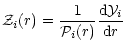 |
|
|
(A.1) |
resulting in the system
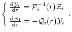 |
|
|
(A.2) |
It is possible
to reduce this system to a new one, where the two equations are
coupled only in the amplitude equation, leaving a single phase equation
to determine the eigenfrequencies.
This is accomplished by using polar coordinates (phase transformation),
 |
|
|
(A.3) |
where
 ,
is the amplitude of the wave function
,
given by
,
is the amplitude of the wave function
,
given by
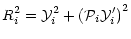 |
|
|
(A.4) |
and
 ,
the phase of the wave function
,
given by
,
the phase of the wave function
,
given by
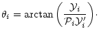 |
|
|
(A.5) |
Solving the system (A.2) for Ri and ,
yields
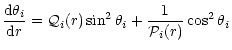 |
|
|
(A.6) |
and
![$\displaystyle R_i
=R_{i,{\rm o}}\exp{\left[
\frac{1}{2}
\int_{r_{\rm o}}^r
\lef...
...r) } - {\cal Q}_i(r) \right)
\sin{\left(2\theta_i\right)} \; {\rm d}r
\right]}.$](/articles/aa/full/2001/27/aah2247/img211.gif) |
|
|
(A.7) |
Equations (A.6) and (A.7) are called the phase associated system.
Each solution of the original self-adjoint differential
Eq. (29) is determined up
by two constants:
the initial amplitude
 and the initial phase
 ,
where
,
where  corresponds to the endpoint
where the boundary condition is applied. The change of the initial phase
,
corresponds to multiply the solution
,
by a constant factor; thus, the zeros of the wave function
can be located by studying the differential Eq. (A.6).
In this sense,
this transformation preserves the zeros of the original wave function,
and their respective location.
The eigenmodes can be determined by the solution of Eq. (A.6)
with the convenient boundary conditions.
We remember that this analysis is applied to the linear adiabatic non-radial
oscillations and consequently the amplitude of waves
can be determined up to an arbitrary constant.
corresponds to the endpoint
where the boundary condition is applied. The change of the initial phase
,
corresponds to multiply the solution
,
by a constant factor; thus, the zeros of the wave function
can be located by studying the differential Eq. (A.6).
In this sense,
this transformation preserves the zeros of the original wave function,
and their respective location.
The eigenmodes can be determined by the solution of Eq. (A.6)
with the convenient boundary conditions.
We remember that this analysis is applied to the linear adiabatic non-radial
oscillations and consequently the amplitude of waves
can be determined up to an arbitrary constant.
We point out that the transformation of the standard
differential equation into a self-adjoint form
does not conserve necessarily the number of zeros or the location of the original
differential equation. The same remains true for all the transformations
between equivalent differential equations.
However, under the two transformations presented previously
to the differential Eq. (4),
the self-adjoint transformation and the phase transformation,
the number and the location of zeros of the wave function are preserved. In the case of the self-adjoint form it is necessary
to take the convenient formulation, for which the function
,
does not presents zeros in the interval, where the self-adjoint form
is applied.
Furthermore, we point out that the number of zeros of a given eigenfunction is not
a unique way to classify modes (see Sect. 5).
In fact, a classification scheme can be determined independent
of that and the number of zeros can be used to classify
the modes only in some particular cases.
A.2 Local phase properties
The properties of the eigenfunction and of the correspondent
eigenfrequencies can be determined from Eq. (A.6),
with the correspondent boundary conditions.
It is possible to build a graph
for each eigenmode of a given eigenfrequency
and degree l,
where
the variation of the phase with the stellar radius is represented.
We call this the linear phase diagram (see Fig. 4), and
we will return later to this point.
A solution
 of the Eq. (29) has a zero at a point
r=r1 if and only if
of the Eq. (29) has a zero at a point
r=r1 if and only if
 ,
where n is always
an integer.
At each of these points
,
where n is always
an integer.
At each of these points
 and
and
 .
On the propagation regions where
,
this means geometrically that each curve
.
On the propagation regions where
,
this means geometrically that each curve
 in the plane
,
corresponding to a solution
of the differential Eq. (29)
(for a given eigenvalue ), can cross the
in the plane
,
corresponding to a solution
of the differential Eq. (29)
(for a given eigenvalue ), can cross the
 axis
(
axis
(
 )
counterclockwise when
)
counterclockwise when
 ,
and
clockwise when
,
and
clockwise when
 .
The solution
of the Eq. (29)
(or equivalently of the Eq. (A.6)) for a
given interval can lead to one of two possible
cases:
If sgn
.
The solution
of the Eq. (29)
(or equivalently of the Eq. (A.6)) for a
given interval can lead to one of two possible
cases:
If sgn
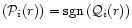 then it has a discrete number of zeros, if any at all.
Alternatively, if
sgn
then it has a discrete number of zeros, if any at all.
Alternatively, if
sgn
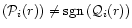 then it has either one zero or no zero at all.
The waves are propagative only, where
sgn
and they are evanescent elsewhere.
In the case of the acoustic propagative region
(
and
)
the phase is increasing with the radius
(
then it has either one zero or no zero at all.
The waves are propagative only, where
sgn
and they are evanescent elsewhere.
In the case of the acoustic propagative region
(
and
)
the phase is increasing with the radius
(
 )
and
in the case of gravity propagative region (
and
)
the phase
is decreasing with the radius (
)
and
in the case of gravity propagative region (
and
)
the phase
is decreasing with the radius (
 ).
In case of pure acoustic modes,
the phase
is always
increasing (
)
in all the interval where the wave is propagative,
and decreasing elsewhere.
This works conversely for the pure gravity modes.
).
In case of pure acoustic modes,
the phase
is always
increasing (
)
in all the interval where the wave is propagative,
and decreasing elsewhere.
This works conversely for the pure gravity modes.
In resume, we can identify a particular phase signature of modes
related with the propagative behavior in a given region. Then
locally a gravity type wave and a acoustic type wave,
propagates
depending upon whether the phase point is
traveling clockwise (gravity or g-modes, where
),
or counterclockwise (acoustic or p-modes, where
),
at points of
,
as r increases.
The global behavior of the eigenmodes is discussed in the Sect. 3.2.
Appendix B: Determination of the boundary conditions in the case of planar approximation
In this section, we present the calculation of the endpoints conditions of
the associated phase system, applied to equations of motion for adiabatic oscillations
when the wavelength is much less than the solar radius, the local effects of spherical
geometry on the dynamic can be ignored (Deubner & Gough 1984,
see also Sect. 2.1.1).
To simplify the determination of the
endpoints of the phase equations, from the
boundary conditions (see Sect. 2.2), we will
consider the phase equations, on the approximation proposed in Sect. 3.4
(Eqs. (51) and (52)).
Furthermore, we will consider only the dominant terms for
and
in the planar approximation, given by Eq. (26),
which are proportional to
 and N2, respectively.
This example is particularly interesting
because the boundary conditions corresponding to that case remain the same
for the other approximations by the fact that the dominant terms
which determine the local behaviour of the phase are
presented in this case. The functions,
and
are given approximately by
and N2, respectively.
This example is particularly interesting
because the boundary conditions corresponding to that case remain the same
for the other approximations by the fact that the dominant terms
which determine the local behaviour of the phase are
presented in this case. The functions,
and
are given approximately by
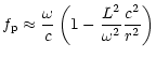 |
|
|
(B.1) |
and
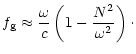 |
|
|
(B.2) |
The boundary condition, of the
function, can be determined
from the boundary conditions of ,
by the Eq. (6)
and the respective boundary conditions for .
The regularity condition in the centre for
is
 |
|
|
(B.3) |
as
.
The boundary condition on the surface, for
is
 |
|
|
(B.4) |
at r=R.
Using the phase transformation (Eq. (A.5)),
![$\displaystyle \cot{\theta_i}
={\rm sgn}({\cal M}_i)\vert{\cal M}_i\vert^{2}\lef...
...r}\ln{\vert{\cal M}_i\vert}
+ \frac{\rm d}{{\rm d}r}\ln{\vert\Psi\vert} \right]$](/articles/aa/full/2001/27/aah2247/img233.gif) |
|
|
(B.5) |
for each one of the descriptions i=1,2.
We observe that for the centre, from the series expansions of equilibrium quantities
we obtain (as
),
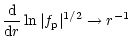 |
|
|
(B.6) |
and
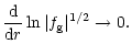 |
|
|
(B.7) |
Under these considerations,
it is possible to determine the initial phase of the associated phase system.
The endpoints for the centre are (
).
In the case of the acoustic description, we obtain
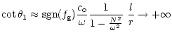 |
|
|
(B.8) |
or
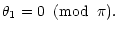 |
|
|
(B.9) |
In the case of the gravity description, we obtain
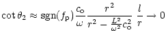 |
|
|
(B.10) |
or
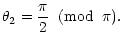 |
|
|
(B.11) |
The endpoints for the surface, can also be calculated for both descriptions.
It is also possible to determine the amplitude boundary conditions,
but they are not interesting to our problem.
At last, it is important to observe that the initial boundary conditions
can be understood in terms of the physical nature of the acoustic
and gravity waves.
-
Cowling, T. G. 1941, MNRAS, 101, 367
In the text
NASA ADS
-
Cox, J. P. 1980, Theory of stellar pulsation (Princeton University Press)
In the text
-
Deubner, F.-L., & Gough, D. O. 1984, ARA&A, 22, 593
In the text
NASA ADS
-
Eckart, C. 1960, Hydrodynamics of Oceans and Atmospheres (Pergamon, London)
In the text
-
Gabriel, M., & Scuflaire, R. 1979, Acta Astron., 29, 135
In the text
NASA ADS
-
Gough, D. O. 1990, Progress of Seismology of the Sun and Stars,
ed. Y. Osaki, & H. Shibahashi (Springer-Verlag, Dordrecht), 283
-
Gough, D. O. 1993, Astrophysical fluid dynamics,
ed. J.-P. Zahn, & J. Zinn-Justin (Elsevier, Amsterdam), 399
In the text
-
Gough, D. O. 1996, The structure of the sun, ed. T. Roca
Cortés (Cambridge University Press), 141
In the text
-
Gough, D. O., & Toomre, J. 1991, ARA&A, 29, 627
NASA ADS
-
Lamb, H. 1932, Hydrodynamics (Cambridge University Press)
In the text
-
Ledoux, P., & Walraven, T. 1958, Handbuch der Physik,
ed. S. Flügge (Springer, New York), 353
In the text
-
Lee, U. 1985, Publ. Astron. Soc. Japan, 37, 262
In the text
-
Lopes, I. P. 2001, MNRAS, 321, 615
In the text
NASA ADS
-
Lopes, I. P. 2000, ApJ, 542, 1071
In the text
NASA ADS
-
Lopes, I. P., & Gough, D. O. 2001, MNRAS, 322, 473
In the text
NASA ADS
-
Lopes, I., Turck-Chiéze, S., Michel, E., & Goupil, M.-J. 1997,
ApJ, 480, 794
In the text
NASA ADS
-
Osaki, Y. 1975, Publ. Astron. Soc. Japan, 27, 237
In the text
NASA ADS
-
Osaki, Y. 1976, Publ. Astron. Soc. Japan, 28, 105
NASA ADS
-
Provost, J., & Berthomieu, G. 1986, A&A, 165, 218
In the text
NASA ADS
-
Prüfer, H. 1926, Mathematische Annalen, 95
In the text
-
Scuflaire, R. 1974, A&A, 36, 107
In the text
NASA ADS
-
Shibahashi, H. 1979, Publ. Astron. Soc. Japan, 31, 87
In the text
NASA ADS
-
Shibahashi, H., & Osaki, Y. 1976a, Publ. Astron. Soc. Japan, 28, 199
In the text
NASA ADS
-
Shibahashi, H., & Osaki, Y. 1976b, Publ. Astron. Soc. Japan, 28, 533
In the text
NASA ADS
-
Smeyers, P., & Tassoul, M. 1988, ApJS, 65, 429
In the text
-
Tassoul, M. 1980, ApJS, 43, 469
In the text
NASA ADS
-
Tassoul, M. 1990, ApJ, 358, 313
In the text
NASA ADS
-
Unno, W., Osaki, Y., Ando, H., Saio, H., & Shibahashi, H. 1989, Nonradial Oscillations of Stars
(University of Tokyo Press)
In the text
-
Vorontsov, S. V. 1991, Sov. Astron. Lett., 35(4), 400
In the text
Copyright ESO 2001
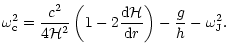
![\begin{figure}
\includegraphics[width=14cm]{2247f1.eps}
\end{figure}](/articles/aa/full/2001/27/aah2247/img69.gif)
![\begin{figure}
\includegraphics[width=14cm]{2247f2.eps}
\end{figure}](/articles/aa/full/2001/27/aah2247/img98.gif)