![[*]](/icons/foot_motif.gif)
A&A 373, 895-898 (2001)
DOI: 10.1051/0004-6361:20010655
Y. Karatas1 - S. Karaali 1 - R. Buser 2
1 - Istanbul University Science Faculty,
Department of Astronomy and Space Sciences,
34452 University-Istanbul, Turkey
2 - Astronomisches Institut der Universität Basel, Venusstr. 7, 4102 Binningen, Switzerland
Received 19 March 2001 / Accepted 2 May 2001
Abstract
The South Galactic pole field SA141 is investigated by using the full calibration tools of RGU photometry. The observed RGU data are reduced to the standard system, and the separation of dwarfs and evolved stars is carried out by an empirical method. Stars are categorized into different metallicity classes and their absolute magnitutes are determined by the corresponding colour-magnitude diagrams. 9 extra-galactic objects have been eliminated from the present stellar statistical treatment.
The local luminosity function agrees with the Gliese (1969) and the partly with the Hipparcos (Jahreiss & Wielen 1997) luminosity function. At the brighter luminosity intervals, the low value of the present observed luminosity function is most probably due to the larger uncertainty in the absolute magnitude determination implied by stars near the main-sequence turnoff. For giants, we found an upper limit,
D*(0) = 6.80, of logarithmic local space density close to the one of Gliese & Jahreiss (1992), i.e.:
 .
.
Key words: Galaxy: structure - stars: luminosity function
The photographic data presented in this paper have been obtained in the context of the re-evaluation program of the Basel RGU three-colour photometric high-latitude survey of the Galaxy, which comprises homogeneous magnitudes and colours for about 20000 stars in a total of fourteen fields distributed along the Galactic meridian through the Galactic center and the sun (Buser & Rong 1995). While the ensemble of the full survey data are being analysed by comprehensive modelling of the density, luminosity, and metallicity distributions of the different Galactic population components (Buser et al. 1998, 1999, henceforth BRK; Rong et al. 2001), the data in each individual field are being used as well for a detailed study of the luminosity function(s) resulting from extensions of the classical three-colour method originally developped by Becker (Ak et al. 1998). In the present paper, recovery of the local luminosity function as given by the Gliese (1969) and/or Hipparcos (Jahreiss & Wielen 1997) data is barely possible, however, because the large scatter in the observed two-colour observations seriously distorts the derivation of the intrinsic properties (such as the dwarf/giant nature, the metallicity, and the absolute magnitude) of the individual stars in this field.
The central coordinates of the field with size 1.92 square-degrees are:

![\begin{figure}
\par\includegraphics[width=8.8cm,clip]{fig1.eps}
\end{figure}](/articles/aa/full/2001/27/aa1273/img19.gif) |
Figure 1: Colour-magnitude diagram for the field SA141 down to the limiting magnitude, G=16.50. |
| Open with DEXTER | |
| Apparent | G | G-R | U-G |
| magnitude interval | |||
| <10 |  0.01
0.01 |
0.01 |
0.01 |
| 10 - 11 | 0.01 | 0.02 | 0.01 |
| 11 - 12 | 0.02 | 0.04 | 0.04 |
| 12 - 13 | 0.02 | 0.02 | 0.04 |
| >13 | 0.02 | 0.02 | 0.04 |
Following standard procedures (Buser 1988), the standard stars are plotted on diagrams  versus
 ,
,
 versus
,
and
versus
,
and  versus
 ,
in order to check on and account for possible colour-equations in bringing the observed data to the standard system. In this notation, ,
,
and
are the differences between standard (i.e., transformed from UBV:
,
in order to check on and account for possible colour-equations in bringing the observed data to the standard system. In this notation, ,
,
and
are the differences between standard (i.e., transformed from UBV:  ,
,
 ,
and
,
and  )
and observed magnitudes (i.e., derived from the characteristic curves:
)
and observed magnitudes (i.e., derived from the characteristic curves:
 ,
,
 ,
and
,
and
 ), and
and
are the observed colour-indices. In fact, Fig. 2 (given in electronic format) shows no indication of a colour-equation. Therefore, all the observed RGU magnitudes and colours used in this paper have been adopted as standard intrinsic data.
), and
and
are the observed colour-indices. In fact, Fig. 2 (given in electronic format) shows no indication of a colour-equation. Therefore, all the observed RGU magnitudes and colours used in this paper have been adopted as standard intrinsic data.
The G-fractioned two-colour diagrams are given in Fig. 3 (in electronic format). The number of stars which occupy the relatively metal-rich region,
![${\rm [M/H]}>-0.25$](/articles/aa/full/2001/27/aa1273/img32.gif) dex, is relatively small, and the opposite is the case for metal-poor stars - which is expected for a pole-field. However, at the same time, it is difficult to explain why a considerable number of stars (even in apparently bright G-intervals) should have metallicities
dex, is relatively small, and the opposite is the case for metal-poor stars - which is expected for a pole-field. However, at the same time, it is difficult to explain why a considerable number of stars (even in apparently bright G-intervals) should have metallicities
![${\rm [M/H]}<-3.00$](/articles/aa/full/2001/27/aa1273/img33.gif) dex.
Comparison of the present field with the Minnesota University survey charts reveals that 9 of these stars are in fact extra-galactic objects (galaxies or quasars), six of which are extremely metal-poor, i.e.:
dex.
These objects have thus been excluded from the present statistical investigation.
dex.
Comparison of the present field with the Minnesota University survey charts reveals that 9 of these stars are in fact extra-galactic objects (galaxies or quasars), six of which are extremely metal-poor, i.e.:
dex.
These objects have thus been excluded from the present statistical investigation.
Following the conclusions of some earlier studies of high-latitude fields (Karaali 1992; Karaali et al. 1997; Ak et al. 1998), the difficult separation of the unevolved and the evolved stars was again attempted by assuming that, for apparent magnitudes brighter than G=16.00 mag, stars which according to their positions in the two-colour diagram could be identified as dwarfs with assigned absolute magnitudes fainter than M(G)=6.0 mag, are however most likely evolved subgiant or giant stars with correspondingly brighter absolute magnitudes.
Within each of these two stellar evolutionary categories,
metallicity and absolute magnitude estimates have then been derived for
each star from its
observed position in the appropriate metallicity-calibrated two-colour
and colour-magnitude
diagrams given by Buser & Fenkart (1990) and by Buser et al.
(2000), respectively. Note that this procedure also
allows each star to be
assigned to one of the Galactic population components, which may be
tentatively
defined by the following approximate metallicity ranges: Population I,
![$-0.25<[{\rm M/H}]\leq+0.50$](/articles/aa/full/2001/27/aa1273/img34.gif) ,
Intermediate Population II,
,
Intermediate Population II,
![$-1.00<[{\rm M/H}]\leq-0.25$](/articles/aa/full/2001/27/aa1273/img35.gif) ,
and
Extreme Population II,
,
and
Extreme Population II,
![$[{\rm M/H}]\leq-1.00$](/articles/aa/full/2001/27/aa1273/img36.gif) dex.
dex.
Finally, stars lying in an area of the two-colour diagram which is outside the
calibration grid and which is suggestive of extremely low metallicity
![$[{\rm M/H}]\leq-3.00$](/articles/aa/full/2001/27/aa1273/img37.gif) dex, are initially all assigned to the Extreme Population II, adopting
dex, are initially all assigned to the Extreme Population II, adopting
![$[{\rm M/H}]=-3.00$](/articles/aa/full/2001/27/aa1273/img38.gif) dex as an upper limit of their metallicity, which then also determines their absolute
magnitudes from the corresponding colour-magnitude diagram.
dex as an upper limit of their metallicity, which then also determines their absolute
magnitudes from the corresponding colour-magnitude diagram.
The logarithmic space densities
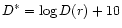 for stars of all populations, i.e.:
Population I, Intermediate Population II, and Extreme Population II are given in Tables 2 and 3 for dwarfs and giants, respectively. Here,
for stars of all populations, i.e.:
Population I, Intermediate Population II, and Extreme Population II are given in Tables 2 and 3 for dwarfs and giants, respectively. Here,
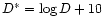
 ,
N being the number of stars, found in the partial volume
,
N being the number of stars, found in the partial volume
 ,
which is determined by the limiting distances r1 and r2, and apparent field-size in square degrees
,
which is determined by the limiting distances r1 and r2, and apparent field-size in square degrees  ,
i.e.:
,
i.e.:
 .
As usual, density functions are then given in the form of histograms,with density plotted as a solid dot at the centroid distance,
.
As usual, density functions are then given in the form of histograms,with density plotted as a solid dot at the centroid distance,
![$\bar{r}=[(r^{3}_{1}+r^{3}_{2})/2]^{1/3}$](/articles/aa/full/2001/27/aa1273/img42.gif) ,
of the corresponding partial volume,
(see, e.g., Del Rio & Fenkart 1987; Fenkart & Karaali 1987).
,
of the corresponding partial volume,
(see, e.g., Del Rio & Fenkart 1987; Fenkart & Karaali 1987).
 |
(2,3] | (3,4] | (4,5] | (5,6] | (6,7] | (7,8] | (8,9] | (9,10] | ||
| r1-r2 |
|
 |
N D* | N D* | N D* | N D* | N D* | N D* | N D* | N D* |
| 0.00-0.40 | 1.23 (4) | 0.32 | 01 5.91 | 07 6.76 | 19 7.19 | 27 7.34 | 55 7.65 | 56 - | 18 - | |
| 0.00-1.58 | 7.76 (5) | 1.26 | 04 4.71 | |||||||
| 0.40-0.63 | 3.67 (4) | 0.54 | 02 5.74 | 02 574 | 15 6.61 | 29 6.90 | 6 - | |||
| 0.40-1.00 | 1.83 (5) | 0.81 | 10 5.74 | |||||||
| 0.63-1.00 | 1.46 (5) | 0.86 | 02 5.14 | 02 5.14 | 33 6.35 | 10 5.84 | ||||
| 1.00-1.58 | 5.81 (5) | 1.36 | 03 4.71 | 13 5.35 | 06 5.01 | |||||
| 1.00-2.51 | 2.96 (6) | 2.04 | 03 4.02 | |||||||
| 1.58-2.51 | 2.31 (6) | 2.15 | 04 4.24 | 02 3.94 | 02 3.94 | |||||
| 2.51-3.98 | 9.21 (6) | 3.40 | 10 4.04 | 03 3.51 | ||||||
| 3.98-6.31 | 3.67 (7) | 5.40 | 03 2.91 |
The comparison of the density functions with the best-fitting model density gradients predicted by BRK are matched to the observed density profiles in order to extrapolate the local stellar space densities. There is a good agreement between the model gradients and the observed density histograms (Fig. 4, in electronic format). However, there are some significant differences when local densities are considered: the luminosity function resulting from comparison of the observed histograms with the best fitting BRK-model gradients agrees with the Gliese (1969) luminosity function only for the absolute
magnitude intervals
 ,
,
 ,
and
,
and
 ,
if a relatively high local logarithmic space density for giants,
D*(0)=6.80, is adopted. For
,
if a relatively high local logarithmic space density for giants,
D*(0)=6.80, is adopted. For
 ,
the observed luminosity function is lower than the Gliese standard (1969), while the opposite is true for
,
the observed luminosity function is lower than the Gliese standard (1969), while the opposite is true for
 (Table 4 and Fig. 5).
| r1-r2 |
|
|
N D* |
| 0.00-2.51 | 3.09 (6) | 1.99 | 06 4.29 |
| 2.51-3.98 | 9.21 (6) | 3.40 | 08 3.94 |
| 3.98-6.31 | 3.67 (7) | 5.40 | 12 3.51 |
| 6.31-10.0 | 1.46 (8) | 8.55 | 21 3.16 |
| 10.00-15.85 | 5.81 (8) | 13.56 | 10 2.24 |
| 15.85-19.95 | 7.72 (8) | 18.13 | 02 1.41 |
| 19.95-25.12 | 1.54 (9) | 22.83 | 03 1.29 |
|
|
(2,3] (3,4] (4,5] (5,6] (6,7] (7,8] |
| All Populations | 6.68 6.43 6.69 7.33 7.65 8.16 |
| s() |
0.27 0.11 0.39 0.54 0.28 0.00 |
| Gliese (1969) | 6.78 7.18 7.41 7.52 7.48 7.42 |
The low value of the present observed luminosity
function at the brighter luminosity intervals is most probably due to the
larger uncertainty in the absolute magnitude determination implied for stars near the main-sequence turnoff at about B-V=0.4 mag, corresponding to
 mag (Gilmore 1984; Fenkart & Karaali 1987), and the high value for the interval
is probably due to the scattering of stars to the metal-poor region in the two-colour diagrams.
mag (Gilmore 1984; Fenkart & Karaali 1987), and the high value for the interval
is probably due to the scattering of stars to the metal-poor region in the two-colour diagrams.
![\begin{figure}
\par\includegraphics[width=8.8cm,clip]{fig5.eps}
\end{figure}](/articles/aa/full/2001/27/aa1273/img52.gif) |
Figure 2:
Luminosity function for SA141 resulting from comparison of
observed combined histograms with best-fitting BRK-model gradient ( ), and confronted to Gliese's (1969) ( ), and confronted to Gliese's (1969) ( ), and Hipparcos' (Jahreiss &
Wielen 1997) (H) local luminosity functions. ), and Hipparcos' (Jahreiss &
Wielen 1997) (H) local luminosity functions. |
| Open with DEXTER | |
We have shown that the observed stellar luminosity function in SA 141 agrees with the local luminosity function as given by the Gliese and/or the Hipparcos catalogs only for three intervals, i.e.:
,
,
and
,
whereas there are significant differences for the other three intervals, i.e.:
 ,
,
 ,
and
.
On the other hand, if the Gliese and/or Hipparcos local luminosity functions are given as input functions for detailed modelling, the best-fitting model calculations of the statistical observed colour-magnitude distribution functions provide resulting density and metallicity structures of the different Galactic components which are in excellent agreement with independent survey results (Buser et al. 1998, 1999; Rong et al. 2001). We thus conclude that, depending on the particular field and on the presence of considerable scatter in the data, the "classical'' derivation of the luminosity function, which proceeds by evaluating the stellar properties on a star-by-star basis, is bound to fall short of properly accounting for the multiple interdependencies between these properties of the stellar individuals in case of significant mix of populations along the line of sight - in perfect agreement with both the prediction made by Buser & Fenkart (1990) and the conclusion found by Ak et al. (1998).
,
and
.
On the other hand, if the Gliese and/or Hipparcos local luminosity functions are given as input functions for detailed modelling, the best-fitting model calculations of the statistical observed colour-magnitude distribution functions provide resulting density and metallicity structures of the different Galactic components which are in excellent agreement with independent survey results (Buser et al. 1998, 1999; Rong et al. 2001). We thus conclude that, depending on the particular field and on the presence of considerable scatter in the data, the "classical'' derivation of the luminosity function, which proceeds by evaluating the stellar properties on a star-by-star basis, is bound to fall short of properly accounting for the multiple interdependencies between these properties of the stellar individuals in case of significant mix of populations along the line of sight - in perfect agreement with both the prediction made by Buser & Fenkart (1990) and the conclusion found by Ak et al. (1998).
Acknowledgements
We would like to thank the Swiss National Science Foundation for financial support, and to the University of Minnesota for providing us with its APS on-line catalogues for the field investigated in this study.
![\begin{figure}
\centering
\includegraphics[width=8.8cm,clip]{ms1273f2.ps}
\end{figure}](/articles/aa/full/2001/27/aa1273/img55.gif) |
Figure 2: Differences between the standard and observed apparent magnitudes versus observed colour indices. There is no indication of any colour equation in the data. |
| Open with DEXTER | |
![\begin{figure}
\includegraphics[width=18cm,clip]{ms1273f3.ps}
\end{figure}](/articles/aa/full/2001/27/aa1273/img56.gif) |
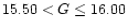
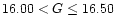
Figure 3:
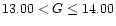
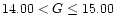
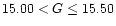
Two-colour diagrams for six consecutive apparent G-magnitude intervals, i.e.:
a)
 ,
b) ,
b)
 ,
c) ,
c)
 ,
d) ,
d)
 ,
e) ,
e)
 ,
and f) ,
and f)
 .
The superposed grid of iso-metallicity lines for dwarf stars is based on theoretical
model atmosphere calculations (Buser & Fenkart 1990), and has been used for
initially classifying the stars into coarse metallicity classes: ()
Population I main sequence,
( .
The superposed grid of iso-metallicity lines for dwarf stars is based on theoretical
model atmosphere calculations (Buser & Fenkart 1990), and has been used for
initially classifying the stars into coarse metallicity classes: ()
Population I main sequence,
( )
Intermediate Population II main sequence, ( )
Intermediate Population II main sequence, ( )
Extreme Population II main sequence,
( )
Extreme Population II main sequence,
( )
late-type giants. 9 extra-galactic objects are marked with plus signs (+). )
late-type giants. 9 extra-galactic objects are marked with plus signs (+). |
| Open with DEXTER | |
![\begin{figure}
\includegraphics[width=13cm,clip]{ms1273f4.ps}
\end{figure}](/articles/aa/full/2001/27/aa1273/img57.gif) |
Figure 4:
Logarithmic space-density histograms for stars of all populations, within the limiting apparent
magnitude of different M(G) intervals. a) (2, 3], b) (3, 4], c) (4, 5], d) (5, 6], e) (6, 7], f)
(7, 8], and g) for giants. ()
centroid-distances within the limits of completeness for
comparison with the BRK model-gradient (thin curve). |
| Open with DEXTER | |
 ,
where
,
where
 ,
N being the number of stars in the partial volume
,
N being the number of stars in the partial volume