A&A 373, 950-959 (2001)
DOI: 10.1051/0004-6361:20010681
R. Gális 1 - L. Hric 2 - P. Niarchos 3
1 - Faculty of Sciences, University of P. J. Safárik,
Moyzesova 16, 041 54 Kosice
The Slovak Republic
2 -
Astronomical Institute of the Slovak Academy of Sciences,
059 60 Tatranská Lomnica,
The Slovak Republic
3 -
Department of Astrophysics, Astronomy and Mechanics, Faculty of Physics, University of Athens, Panepistimiopolis, 15784 Zografos,
Athens, Greece
Received 11 December 2000/ Accepted 12 April 2001
Abstract
An analysis of UBV photoelectric photometry for the eclipsing binary KW Per based on new observational data is presented. The light changes are not only due to eclipses, but also to activity in the system.
The U, B and V light curves are analyzed by the Binary Maker 2.0 and Wilson-Devinney codes to derive the geometrical and physical parameters of the system. Since the O'Connell effect is present on the light curves in the three colours, the unperturbed parts of the light curves are considered to represent the quiet stage of the system, in contrast to the active stage which is represented by the perturbed parts of the light curves.
The discussion about the evolutionary status of the system indicates that the secondary component of the binary system is an evolved star and the primary is a MS star.
Key words: binaries: eclipsing - techniques: photometric - stars: individual: KW Per
A new group, the near-contact binaries, with similar characteristics to the A type of W UMa eclipsing binaries, has been established by Shaw (1990). They have orbital periods less than one day, the components show tidal deformation and the facing surfaces are less than 0.1 orbital radius apart. Most of the systems have one component at or near its Roche lobe. The spectral type of the hot component is A or F, while that of the cooler one is a spectral type or two later. This similarity of features suggests that the near-contact binaries could be the missing link between detached binaries and W UMa systems, at least of A type. Evolutionary possibilities concerning the near-contact binaries have been discussed by Hilditch et al.(1988). While in 1990 the whole group of near-contact binaries consisted of 40 members, in 1994, when Shaw established the subgroup of under-massive stars, besides the existing ones of V1010 Ophiuchi and FO Virginis (Shaw 1994), the list contained 130 systems. A common characteristic in the light curves of near-contact systems is the O'Connell effect. Most of the near contact systems show maximum I (phase 0.25) higher than maximum II (phase 0.75). In such a case, cool interstellar matter absorbing a part of luminosity around the phase 0.75 could be invoked to explain the variations. The supplementary luminosity (close to the phase 0.25) of the mass stream from the hot component is the second possibility to explain the behaviour of the light curve.
KW Per has been included in the list of near-contact binaries by Shaw (1994)
based on its features, but with a note that the existing observational
material does not allow a precise classification of the system. However, only half a dozen papers discuss this interesting star. The first ephemeris was determined by Böhme (1976) on the basis of 208 photographic plates taken in B colour at the Sonneberg Observatory in the years 1967-1974. The data have been extended by published observations (Bamberg Veröff. 5, No. 15, BBSAG-Bull 25, 26 and Brno Publ. 6, 9, 17) and the resulting ephemeris is :
| Star | V = KW Per | S1 | Ch | S2 | S5 |
| HD | 012280 | 232571 | 12089 | 12072 | |
| BD | +52 483 | +51 468 | +52 471 | +52 486 | +52 484 |
|
|
|
|
|
|
|
|
|
|
|
|
|
|
| spectrum | A2 (GCVS) | F5 (GSC) | K2 (GSC) | A0 (GSC) | G5 (GSC) |
| U | 8.64 | 9.77 |
|
|
|
| B | 8.64 |
|
|
||
| V | 8.20 |
|
|
One time of primary minimum of KW Per has been published by Braune et al. (1981) on the basis of visual observations. Two times of minima, derived from photoelectric UBV observations, have been published by Faulkner (1986). Hanzl (1990) published one time of primary minimum based on photoelectric observations. The next, mostly visual, times of minima have been adopted from Supplemento ad Annuario Cracoviense (SAC 69, 70) and from the B.R.N.O. database (Zejda 2000), in total, 246 observations.
The system KW Per is included in the Catalogue of binaries by Giuricin et al. (1983) among the evolved systems with unclear nature. Two other objects (PX Car and EP Aur), recorded in the 8-member subgroup, are in the list of near-contact binaries together with KW Per (Shaw 1994).
The observational material used in this paper was taken at the Observatories
of the Astronomical Institute of the Slovak Academy of Sciences at the Stará Lesná (SL) and Skalnaté Pleso (SP), as well as at the Astronomical Station of the National Observatory of Athens at Kryonerion (KR). The observations were carried out in 25 runs (24 nights) during the period from December 4th 1996 to November 25th 1998 in 112 hours of pure observational time. For the sake of quality for the next light curve analysis only 16 excellent nights were used.
| Julian Date | Date | Obs. | Obsrv. | Duration | Phase int.* | Comp. | Ext.Coeff.** | O.K. |
| Note | ||
| -2400000 | h m s | U | B | V | ||||||||
| 50426 | 08/12/96 | SL | Ga | 6 59 0 | 0.17 - 0.48 | S1(S2,Ch,S5) | 0.66 | 0.36 | 0.21 | No | 68 | 1 |
| 50520 | 12/03/97 | SL | Ga, Hr | 3 49 17 | 0.02 - 0.19 | S2(S5) | 0.74 | 0.42 | 0.26 | Yes | 64 | |
| 50735 | 13/10/97 | SL | Ga | 3 11 57 | 0.84 - 0.98 | S2(S5) | 0.49 | 0.18 | 0.09 | No | 52 | |
| 50745 | 23/10/97 | SL | Ga | 1 41 53 | 0.82 - 0.90 | S2(S5) | - | - | - | No | 10 | 2 |
| 50750 | 28/10/97 | SL | Ga | 4 39 58 | 0.22 - 0.43 | S2(S1,S5) | 0.69 | 0.37 | 0.21 | No | 74 | |
| 50799 | 16/12/97 | SL | Ga | 9 40 37 | 0.57 - 1.00 | S2(S5) | 0.63 | 0.33 | 0.20 | Yes | 146 | |
| 50838 | 24/01/98 | SL | Ga | 0 59 6 | 0.43 - 0.46 | S2(S5) | - | - | - | No | 10 | 2 |
| 50846 | 01/02/98 | SL | Ga | 4 27 5 | 0.03 - 0.21 | S2(S5) | 0.56 | 0.26 | 0.13 | No | 70 | |
| 51095 | 08/10/98 | Kr | Ga,Hr | 3 32 55 | 0.72 - 0.84 | S2(S5) | 0.66 | 0.37 | 0.26 | No | 30 | |
| 51096 | 09/10/98 | Kr | Ga,Hr | 7 37 57 | 0.61 - 0.94 | S2(S5) | 0.69 | 0.42 | 0.28 | Yes | 152 | 3 |
| 51104 | 17/10/98 | Kr | Ga,Hr | 4 31 4 | 0.07 - 0.26 | S2(S5) | 0.80 | 0.47 | 0.29 | No | 101 | |
| 51105 | 18/10/98 | Kr | Ga,Hr | 8 49 18 | 0.23 - 0.62 | S2(S5) | 0.58 | 0.29 | 0.15 | Yes | 197 | 3 |
| 51106 | 19/10/98 | Kr | Ga,Hr | 5 55 22 | 0.43 - 0.68 | S2(S5) | 0.63 | 0.33 | 0.23 | Yes | 129 | 3 |
| 51107 | 20/10/98 | Kr | Ga,Hr | 2 27 4 | 0.45 - 0.55 | S2(S5) | - | - | - | No | 52 | |
| 51142 | 24/11/98 | SL | Ga,Hr | 8 39 2 | 0.92 - 0.29 | S2(S5) | 0.84 | 0.50 | 0.31 | No | 224 | |
| 51143 | 25/11/98 | SL | Ga,Hr | 4 2 53 | 0.93 - 0.11 | S2(S5) | - | - | - | No | 108 | |
| * The phases have been computed according to the ephemeris published in GCVS (Kholopov et al. 1985). | ||||||||||||
| ** The columnO.K.indicates use of the seasonal extinction coefficients(No)or the extinction coefficients for given night(Yes). | ||||||||||||
| Notes: | 1 - the observation consists of two parts, | |||||||||||
| 2 - the observation is too short, | ||||||||||||
| 3 - the observation has been used for the determination of the new seasonal extinction coefficients. | ||||||||||||
Comparison stars were chosen from the electronic catalogue of photometric data GCPD by Mermilliod et al. (1997). The star HD 012280 (Oja 1985) was used as comparison
(S1) and HD 232571 (Scharlach & Craine 1983) as the check one. Since both stars are far from the variable, the stars HD 12089 (S2) and HD 12072
(S5) close to the variable were chosen as the comparisons. The new comparisons had not published UBV magnitudes, therefore we performed the cross measurements of all comparison stars during 4 nights and the resulting values are given in Table 1. This table contains designations, equatorial coordinates, proper motions and spectral types for variable as well as for all comparison stars. The mutual comparison of resulting values suggests that all comparison stars are not variable on a short as well as long-time scale respectively. All observations of comparison stars have been transformed into the international system of magnitudes.
The accuracy of the resulting values is a few hundredths of international UBV magnitudes and the error increases up from V towards B and U colour.
Seasonal extinction coefficients have been used in the reduction of observations except in the case of very good atmospheric conditions, when the coefficients of the running night have been adopted. The individual observations are given in Table 2, which contains Julian date, date of observation, observatory, observers, duration of the observation, phase interval,
comparison stars, resulting extinction coefficients and number of observational
points in each filter. The last column in the table describes the character of
observations. A total of 1196 observational points in U, 1292 in B and 1295 in V filter have been obtained.
The mean error of observations in B and V is the same
(
![]() and
and
![]() ,
and the mean
error in U colour is rather larger (
,
and the mean
error in U colour is rather larger (
![]() ).
).
![\begin{figure}
\par\includegraphics[width=8.7cm,clip]{MS10549f1.eps} \end{figure}](/articles/aa/full/2001/27/aa10549/img25.gif) |
Figure 1: Phase diagram of the light curve of KW Per in U colour. |
| Open with DEXTER | |
![\begin{figure}
\par\includegraphics[width=8.7cm,clip]{MS10549f2.eps} \end{figure}](/articles/aa/full/2001/27/aa10549/img26.gif) |
Figure 2: Phase diagram of the light curve of KW Per in B colour. |
| Open with DEXTER | |
The individual observations are depicted in phase diagrams for each colour
U, B and V, while each night is distinguished by the shift in magnitude and by
Julian date (Figs. 1, 2 and 3).
![\begin{figure}
\par\includegraphics[width=8.7cm,clip]{MS10549f3.eps} \end{figure}](/articles/aa/full/2001/27/aa10549/img27.gif) |
Figure 3: Phase diagram of the light curve of KW Per in V colour. |
| Open with DEXTER | |
The light curves in the phase diagrams are very well covered by observational
points and, for particular phase intervals, about the same number of observational points in each filter (![]() 60 points per 0.05 of phase interval) is secured, which is a prerequisite for accurate analysis of KW Per.
60 points per 0.05 of phase interval) is secured, which is a prerequisite for accurate analysis of KW Per.
The rather homogeneous covering of the light curves in all colours justifies performing the statistical analysis of mean errors of individual observational points.
The whole phase interval was divided into 20 subintervals with a width of
![]() ,
while all intervals were overlapped with the shift in phase
(
,
while all intervals were overlapped with the shift in phase
(
![]() ). Polynomials of higher orders have been used for fitting, while the character and the shape of the light curves have been taken into account.
). Polynomials of higher orders have been used for fitting, while the character and the shape of the light curves have been taken into account.
The graphical representation of the previous statistical analysis is shown in
Fig. 4.
![\begin{figure}
\par\includegraphics[width=8.8cm,clip]{MS10549f4.eps} \end{figure}](/articles/aa/full/2001/27/aa10549/img31.gif) |
Figure 4: The phase dependence of mean error of one observational point. |
| Open with DEXTER | |
The observations of KW Per show that the ephemeris published in the literature does not agree, as it can be seen in the phase diagram in all three colours (Figs. 1, 2 and 3). This behaviour has drawn our attention to the analysis of times of minima.
Two times of primary and three times of secondary minima have been secured from our observations. All the available photoelectric, photographic as well as visual times of primary minima have also been adopted from literature. In this way, 266 times of minima have been collected and are displayed in Fig. 5, while the photoelectric times of minima are enhanced.
![\begin{figure}
\par\includegraphics[width=8.8cm,clip]{MS10549f5.eps} \end{figure}](/articles/aa/full/2001/27/aa10549/img39.gif) |
Figure 5: (O-C) diagram of all available times of minima of KW Per (The ephemeris from GCVS (Kholopov et al. 1985) was used for determination of (O-C) values. |
| Open with DEXTER | |
| Epoch | JDhel. | (O-C) [d] | Type of obs. | Ref. |
| 4243 | 46355.6644 | 0.00114 | pe-BV | Faulkner (1986) |
| 4332 | 46438.5455 | 0.00021 | pe-BV | Faulkner (1996) |
| 5381 | 47415.4410 | 0.00518 | pe-B | Hanzl (1990) |
| 5381 | 47415.4410 | 0.00518 | pe-U | Hanzl (1990) |
| 5381 | 47415.4417 | 0.00588 | pe-V | Hanzl (1990) |
| 9343.5 | 51105.5508 | 0.00184 | pe-U, sec. | this paper |
| 9343.5 | 51105.5520 | 0.00301 | pe-B, sec. | this paper |
| 9343.5 | 51105.5541 | 0.00508 | pe-V, sec. | this paper |
| 9344.5 | 51106.4867 | 0.00643 | pe-U, sec. | this paper |
| 9344.5 | 51106.4863 | 0.00603 | pe-B, sec. | this paper |
| 9344.5 | 51106.4872 | 0.00693 | pe-V, sec. | this paper |
| 9345.5 | 51107.4181 | 0.00662 | pe-U, sec. | this paper |
| 9345.5 | 51107.4235 | 0.01201 | pe-B, sec. | this paper |
| 9345.5 | 51107.4205 | 0.00900 | pe-V, sec. | this paper |
| 9383 | 51142.3411 | 0.00740 | pe-U, prim. | this paper |
| 9383 | 51142.3404 | 0.00668 | pe-B, prim. | this paper |
| 9383 | 51142.3406 | 0.00692 | pe-V, prim. | this paper |
| 9384 | 51143.2728 | 0.00784 | pe-U, prim. | this paper |
| 9384 | 51143.2731 | 0.00815 | pe-B, prim. | this paper |
| 9384 | 51143.2732 | 0.00828 | pe-V, prim. | this paper |
| Type of observation: | ||||
| pe-BV - photoelectric, average value from filters B and V | ||||
| pe-U - photoelectric in filter U | ||||
| pe-B - photoelectric in filter B | ||||
| pe-V - photoelectric in filter V |
One can see that particular values are fraught with large errors due to the huge scatter, mostly in visual data. The relevant sums of the squares of the residuals are very similar for both fits , therefore it is impossible to choose the better one. However, we are not able to decide whether inaccurate
JD
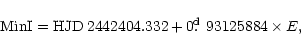
![]() and period P values have been derived or the changes of the orbital period in the system plays some role. We assume that the problem can be solved only by a new period determination. Doing so, a new period
and period P values have been derived or the changes of the orbital period in the system plays some role. We assume that the problem can be solved only by a new period determination. Doing so, a new period
![]() ,
and a new ephemeris is found:
,
and a new ephemeris is found:
Nevertheless the change of orbital period of this system is not excluded. The activity analysis of the system KW Per suggests that mass transfer between components could be present. Such behaviour leads to changes of the orbital period (see Sect. 7).
All observational data in the form of phase and magnitude, are collected in Table 4 (available only in electronic form).
The shape of the light curve does not agree with the
![]() type as was published by Brancewicz & Dworak (1980) and by Kholopov et al. (1985). It seems that a classification of
Algol type is more reliable.
type as was published by Brancewicz & Dworak (1980) and by Kholopov et al. (1985). It seems that a classification of
Algol type is more reliable.
![\begin{figure}
\par\includegraphics[width=8.8cm,clip]{MS10549f6.eps} \end{figure}](/articles/aa/full/2001/27/aa10549/img46.gif) |
Figure 6: The synthetic light curves derived by parameters for mode 2 and 5 with normal points used in light curve analysis with synthetic light curves derived by parameters published by Brancewicz & Dworak (1980). |
| Open with DEXTER | |
In order to determine the physical and geometrical parameters of KW Per, the Binary Maker 2.0 program (Bradstreet 1993) and the 1996 version of the Wilson-Devinney (Wilson 1990) code were used. Before the analysis, a check of the published A2 spectral type of the primary component, on the basis of our observational material, was made. Two methods have been applied.
We have derived intrinsic color indices (U-B)0 and (B-V)0
from the observed ones (
(U-B) = 0.27 and
(B-V) = 0.25) by knowing roughly the interstellar reddening in the direction to KW Per. The charts of colour excess published by FitzGerald (1968) have been used. For the direction around KW Per the colour excess is
(0.2-0.3) for the distance to 500 pc and
(0.3-0.6) to 1000 pc. The published distance of KW Per, 720 pc
(Shaw 1994), yields, by extrapolation, the value of the colour excess
![]() and the intrinsic colour indices
and the intrinsic colour indices
![]() ,
which correspond to spectral types B8-B9 and A1-A2, respectively (Lang 1992).
The two-colour diagram
,
which correspond to spectral types B8-B9 and A1-A2, respectively (Lang 1992).
The two-colour diagram
![]() ,
created by Lang (1992), was used as the second method. In this way the following intrinsic colour indices of KW Per have been established:
,
created by Lang (1992), was used as the second method. In this way the following intrinsic colour indices of KW Per have been established:
![]() ,
which correspond to spectral type A1-A3. This yields the value of the colour excess
E(B-V) = 0.24The methods mentioned above are only a statistical approach and the resulting broad band of spectral types is due to many causes.
,
which correspond to spectral type A1-A3. This yields the value of the colour excess
E(B-V) = 0.24The methods mentioned above are only a statistical approach and the resulting broad band of spectral types is due to many causes.
| Parameter | BM | WD mode 2 | WD mode 5 | |
| inclination | i |
|
|
|
| radii |
|
0.3500 |
|
|
|
|
0.3414 |
|
|
|
|
|
0.3318 |
|
|
|
|
|
0.3567 |
|
|
|
|
|
0.3403 |
|
|
|
|
|
0.3077 |
|
|
|
|
|
0.2949 |
|
|
|
|
|
0.4229 |
|
|
|
| volumes | V1 | 0.1600 | 0.1565 | |
| V2 | 0.1168 | 0.1211 | ||
| mass-ratio | q | 0.47 |
|
|
| potentials |
|
3.4598 |
|
|
|
|
|
|
|
|
|
|
|
|
|
|
| temperatures | T1 |
|
|
|
| T2 | 5 100K |
|
|
|
| gravity-dark. coeffs. | g1 |
|
|
|
| g2 |
|
|
|
|
| albedos | A1 |
|
|
|
| A2 |
|
|
|
|
| limb-dark. coeffs. |
|
|
|
|
|
|
|
|
|
|
| X1(U) |
|
|
|
|
| X1(B) |
|
|
|
|
| X1(V) |
|
|
|
|
| X2(U) |
|
|
|
|
| X2(B) |
|
|
|
|
| X2(V) |
|
|
|
|
| luminosities | L1U/(L1U+L2U) | 0.9809 |
|
|
| L1B/(L1B+L2B) | 0.9662 |
|
|
|
| L1V/(L1V+L2V) | 0.9399 |
|
|
|
| L2U/(L1U+L2U) | 0.0191 |
|
|
|
| L2B/(L1B+L2B) | 0.0338 |
|
|
|
| L2V/(L1V+L2V) | 0.0601 |
|
|
|
|
|
- | 0.05507 | 0.05583 | |
| BM - Binary Maker 2.0 (Bradstreet 1993) | a - computed from Roche geometry (Wilson 1992) | |||
| WD - Wilson-Devinney | b - fixed, adopted from literature | |||
| c - computed from the other parameters | ||||
The next independent test of the spectral type of the primary component of KW Per was the determination of its temperature by the minimization of sum of the squares of the residuals in the light curve analysis. Five light curve solutions was performed
(the detail explanation see below) for spectral type interval A3-B9 which corresponds to interval of temperatures (8720-10500)K (Lang 1992). Our analysis clearly shown that the sum of the squares of the residuals falls to minimum for the temperature
![]() ,
which corresponds to spectral type A1 (interval A0-A2). This value of the temperature of the primary component of KW Per was used in the next light curve analysis.
,
which corresponds to spectral type A1 (interval A0-A2). This value of the temperature of the primary component of KW Per was used in the next light curve analysis.
As a preliminary step in the light curve analysis, the Binary Maker 2.0 program (Bradstreet 1993) was used. The results showed that the secondary component
![]() fills its Roche lobe, the mass ratio is
M2/M1 = 0.47 and the inclination of the system is
fills its Roche lobe, the mass ratio is
M2/M1 = 0.47 and the inclination of the system is
![]() .
All parameters obtained by Binary Maker 2.0 were used as input parameters into the Wilson-Devinney code (Wilson 1990).
.
All parameters obtained by Binary Maker 2.0 were used as input parameters into the Wilson-Devinney code (Wilson 1990).
The normal points were constructed as the average of observational points by the code ASUSPR prepared by one of us (L.H.), which applies the procedure of running averages. This way 340 normal points in U, 344 in B and 358 in V were formed. They cover rather well the entire phase diagram (see Fig. 6). In the next step, the magnitudes have been converted into light intensities.
With respect to the light behaviour of KW Per, the weights of the normal point have not been produced on the basis of number of observational points. Such a procedure could not take into account real changes of brightness in light curves with respect to the homogeneous covering of light curves in each colour. It seems better to use the results from the statistical analysis of mean errors of individual observational points with phase dependence. The weights of normal points have been computed by the equation
![]() as the integers, while the normalization constant has been
chosen to keep the resulting weights in the interval
as the integers, while the normalization constant has been
chosen to keep the resulting weights in the interval
![]() .
The weights of particular light curves have been determined on the basis of the mean errors of individual observational points in each filter. All three light curves were analysed simultaneously.
.
The weights of particular light curves have been determined on the basis of the mean errors of individual observational points in each filter. All three light curves were analysed simultaneously.
In respect to the uncertainty concerning the classification of the object into the near-contact binaries, three modes have been chosen for the analysis: mode 2 for detached systems, mode 4 for semidetached systems with the primary component filling its Roche lobe and mode 5 for semidetached systems with the secondary component filling its Roche lobe. The spot modeling was not considered during the solution of mean light curves, neither was the third light (l3). The circular orbit and the synchronous rotation of the components have been considered in the final solution. The bolometric albedos, the gravity darkening coefficients as well as limb darkening coefficients
have been fixed in the final solution. The limb darkening coefficients have been interpolated for the given temperature, gravity and colour by using van Hamme (1993) tables. The potentials of primary
![]() and secondary
and secondary
![]() components, the mass ratio (q), the inclination of the orbit (i), the effective temperature of the secondary component (T2) as well as the luminosity of the primary component
(L1U, L1B, L1V) have been adjusted.
components, the mass ratio (q), the inclination of the orbit (i), the effective temperature of the secondary component (T2) as well as the luminosity of the primary component
(L1U, L1B, L1V) have been adjusted.
The final solution yields the following results: for the mode 4 (the primary component fills its Roche lobe) the differential corrections lead to an irrelevant physical solution, while for the mode 2 the solution is very close to the semidetached configuration of the components (mode 5).
The synthetic light curves of KW Per produced by using the parameters for
the modes 2 and 5 respectively, as well as the normal points, are depicted in
Fig. 6. It is worth noting that the synthetic light curves produced by different modes are indistinguishable due to their similarity. All derived physical and geometrical parameters of KW Per with errors, for the modes 2 and 5, are given
in Table 5.
The input parameters produced by the Binary Maker 2.0 code appear in the same Table for comparison. Unfortunately, it is impossible to choose the best solution and both sets of parameters are very close to each other. It is clear that the secondary component fills
![]() % its Roche lobe, which means that the solution of the model converges to a semidetached configuration. We adopted the parameters of mode 5 as a final solution for the subsequent study.
% its Roche lobe, which means that the solution of the model converges to a semidetached configuration. We adopted the parameters of mode 5 as a final solution for the subsequent study.
The majority of the properties as well as the evolutionary status (see below) of KW Per suggest the classification of this system as the near-contact binary. The secondary component fills or is near to its Roche lobe, therefore KW Per can be classified as a member of the FO Vir subgroup. Only the distance of facing surfaces of the components is larger than 0.1 orbital radius. It is important to note that some systems from the list of near-contact binaries (Shaw 1994) do not match this criterion too (for example FO Vir with a distance of facing surfaces of the components of 0.18). It will be probably necessary to establish more exact criteria for including the systems into this class. Therefore the question of classification of KW Per as a near-contact binary is still open.
It is necessary to find the absolute parameters of the components of a binary system in order to establish its evolutionary status. Since no spectroscopic mass-ratio is known, an assumption about the mass of the primary component must be made. The MS star of the effective temperature 9340 K has a mass
![]() (Lang 1992). The resulting absolute parameters of KW Per are given in Table 6.
(Lang 1992). The resulting absolute parameters of KW Per are given in Table 6.
The absolute luminosities can be used to produce absolute bolometric magnitudes
of both components
![]() .
The distance of the object can be derived using the apparent magnitudes. During the time of secondary minimum, the secondary component is practicaly completely eclipsed and we can observe only the primary with a magnitude in V = 10.34. Adopting the bolometric correction for a MS star of the effective temperature
.
The distance of the object can be derived using the apparent magnitudes. During the time of secondary minimum, the secondary component is practicaly completely eclipsed and we can observe only the primary with a magnitude in V = 10.34. Adopting the bolometric correction for a MS star of the effective temperature ![]() (Lang 1992)
BC = - 0.26 and taking into account interstellar absorbtion
AV = 0.79 the resulting distance of KW Per is
(Lang 1992)
BC = - 0.26 and taking into account interstellar absorbtion
AV = 0.79 the resulting distance of KW Per is
![]() ,
which is not in agreement with the published value of 720 pc by Shaw (1990).
,
which is not in agreement with the published value of 720 pc by Shaw (1990).
![\begin{figure}
\par\includegraphics[width=8.6cm,clip]{MS10549f7.eps} \end{figure}](/articles/aa/full/2001/27/aa10549/img137.gif) |
Figure 7: HR diagram (Hilditch et al. 1988) and the position of primary and secondary components of KW Per. |
| Open with DEXTER | |
By comparing our parameters with the average published values we can conclude that the radius and luminosity of the primary agrees with those of a MS star, unlike the secondary component, which has a radius 2 times larger and rather larger luminosity and mass. The secondary component is more evolved and the gained parameters fit well with a giant star of spectral type G4 (Lang 1992). The resulting absolute parameters of both components can be used to understand the evolutionary status of KW Per.
A study of the evolutionary status of near-contact and W UMa-type binaries has been given by Hilditch et al. (1988). In this study the mass-radius, mass-luminosity, total orbital angular momenta J/M5/3 versus mass ratios and HR diagrams have been utilized. The position of the primary as well as the secondary component of KW Per depicted in Fig 7. is in good agreement with our previous suggestions that the primary is a MS star and the secondary is an evolved star. KW Per lies in the angular momentum mass ratio diagram in its upper part, which indicates that the angular momentum loss has not yet been activated and hence the system is still not in contact. The positions of KW Per (mainly of its secondary component) on the diagrams mentioned above are similar to those of the system YY Cet.
The binary system KW Per is in the stage of evolution when mass exchange continues in spite of the growing of the Roche lobe of the secondary component. The star has already left the MS and it is expanding. This results in filling or near-filling of the Roche lobe and mass transfer can continue. The mass transfer cannot be continuous, which can be seen as brightness and spectrum variations. Minor light variations are indeed observed in all three colours.
The statistical analysis of the mean errors of individual observational points
![]() with orbital phase dependence have clearly shown that there are parts of light curves with variability, mostly around phase intervals
with orbital phase dependence have clearly shown that there are parts of light curves with variability, mostly around phase intervals
![]() and
and
![]() .
During these periods, the mean errors of individual observational points exceed the mean error of all observations
.
During these periods, the mean errors of individual observational points exceed the mean error of all observations
![]() in particular filters. We consider such behaviour as activity in the system. In Fig. 8 the phase diagrams of the light curves of KW Per are depicted in such a way that particular nights are
distinguished by gray scale.
It is clearly seen that small variations are present not only during the season but even on very short time-scales (1 night). The fast variations of brightness are evident on the nights of JD 2451105, 2451106 and 2451107, while the variations are most pronounced in the U filter. The largest differences are observed in phase interval
in particular filters. We consider such behaviour as activity in the system. In Fig. 8 the phase diagrams of the light curves of KW Per are depicted in such a way that particular nights are
distinguished by gray scale.
It is clearly seen that small variations are present not only during the season but even on very short time-scales (1 night). The fast variations of brightness are evident on the nights of JD 2451105, 2451106 and 2451107, while the variations are most pronounced in the U filter. The largest differences are observed in phase interval
![]() with amplitude 0.1 mag in U and 0.05 in B and V colours. Moreover, sometimes the light curve is not symmetric, while the maximum in phase 0.25 is higher than the one in phase 0.75. In the following analysis we have tried to explain such peculiar behaviour.
with amplitude 0.1 mag in U and 0.05 in B and V colours. Moreover, sometimes the light curve is not symmetric, while the maximum in phase 0.25 is higher than the one in phase 0.75. In the following analysis we have tried to explain such peculiar behaviour.
![\begin{figure}
\par\includegraphics[width=14.1cm,clip]{MS10549f8.eps} \end{figure}](/articles/aa/full/2001/27/aa10549/img138.gif) |
Figure 8: Phase diagram of light curve of KW Per in U, B and V colours. |
| Open with DEXTER | |
The secondary component of KW Per is a good candidate for a star with spots; nevertheless its contribution to the whole brightness of the system is only 3% in U, 5% in B and 8% in V, therefore the spot model is not adequate to explain the light behaviour. Moreover the amplitude of variations is larger in short wavelengths, which also does not fit the spot idea. The primary component, on the other hand, is too hot to keep cool spots on the surface for a long time.
The best explanation of this behaviour seems to be the existence of circumstellar matter in the system. The darkness of the posterior hemisphere (in the sense of orbital motion) of the primary component or brightness of the posterior hemisphere of the secondary, is due to this matter. An accretion luminosity is a well known phenomenon in eclipsing binaries of Algol type, which can explain very well the asymmetry of light curves of near contact binaries, too (Hilditch 1989; Shaw 1990). In the system of KW Per, the hotter component is inside its Roche lobe, therefore the origin of a spot on the surface of the secondary component is not probable. On the other hand, the solution of the mean light curves has shown that the secondary component fills or almost fills its Roche lobe and mass can be transferred through the Lagrangian point L1 to the surroundings of the primary component. This idea is supported by our results from the analysis of the times of minima. When we assume that the behaviour of the (O-C) diagram is due to the lengthening of the orbital period, then the resulting value is
![]() ,
which is in good agreement with values for other near-contact binaries (Shaw 1990). This change of period corresponds to an accretion rate of
,
which is in good agreement with values for other near-contact binaries (Shaw 1990). This change of period corresponds to an accretion rate of
![]() /year. The mass transfered onto the primary component region can create blobs, clumps and other inhomogeneities which may be responsible for minor light variations in the system. These inhomogeneities look like cool regions around the hot component. This assumption has been used in the quantitative analysis of KW Per.
/year. The mass transfered onto the primary component region can create blobs, clumps and other inhomogeneities which may be responsible for minor light variations in the system. These inhomogeneities look like cool regions around the hot component. This assumption has been used in the quantitative analysis of KW Per.
Due to the fact that it is impossible to get the whole light curve of one cycle
from one observatory, we are not able to study the shape of the real light curve. We have established the extreme light curves in such a way that our observed light curves fall in the interval between both extremes. The extreme light curves have been formed from the observed ones and were been used to study the activity stages of the system. The upper extreme curve (quiet stage) was created from the observations of the following dates: JD 2451096, 2451104, 2451105, 2451143 and the lower one (active stage) from the observations at:
JD 2450735, 2450750, 2450799, 2451106 and 2451142. During the active stage a larger amount of mass than in the quiet stage is transferred to the region around the primary component and this results in a drop of brightness in the light curves, mostly in the U colour. Normal points of the extreme light curves have been produced in the same way as mentioned above and the analysis performed by the Binary Maker 2.0 code (Bradstreet 1993). As input parameters we used those from the solution by the Wilson-Devinney code (Wilson 1992) in
semidetached mode (Mode 5). The regions with lower temperature have been
optimized interactively and the derived parameters are listed in Table 7 for both
quiet and active stages respectively.
| Region | quiescence stage | active stage | ||||||
| No. | b | l | R | T | b | l | R | T |
| 1 |
|
|
|
8593 |
|
|
|
7285 |
| 2 |
|
|
|
8873 |
|
|
|
7472 |
| 3 |
|
|
|
8406 |
|
|
|
7472 |
|
b - latitude, l - longitude, R - angular radius, T - temperature. |
In Fig. 9, the model of KW Per is presented for quiescence as well as for the active stage and for phase 0.15 and 0.90, respectively.
In Fig. 10 the corresponding light curves are shown in U, B and V and for quiet and active stages, respectively. We can conclude that the resulting synthetic light curves fit very well the normal points in both quiet and active stages in each filter. The proposed model of KW Per describes rather well the circumstellar matter in the system.
![\begin{figure}
\par\includegraphics[width=5.7cm,clip]{MS10549f9a.eps}\hspace*{3....
...\hspace*{3.5cm}
\includegraphics[width=5.7cm,clip]{MS10549f9d.eps} \end{figure}](/articles/aa/full/2001/27/aa10549/img151.gif) |
Figure 9: The model of KW Per in quiescence (left) and active stage (right) in phase 0.15 (top) and 0.90 (bottom). |
| Open with DEXTER | |
The results achieved by the quantitative analysis of the activity of KW Per can be summarized as follows: (a) The quantitative analysis confirmed the presence of circumstellar matter around the primary component; (b) during the active stage the individual parts of the circumstellar matter have lower temperatures and larger sizes than in the quiet stage and this is very probably due to a higher rate of transferred matter from the secondary component; (c) the mass transfer rate changes very fast on time scales comparable with the orbital cycle of the system.
In Fig. 11 the new model of KW Per is drawn, together with the inner and outer
Lagrangian surfaces.
![\begin{figure}
\par\includegraphics[width=8.8cm,clip]{MS10549f10.eps} \end{figure}](/articles/aa/full/2001/27/aa10549/img152.gif) |
Figure 10: The synthetic light curves of KW Per for quiescence and active stage with corresponding normal points. |
| Open with DEXTER | |
![\begin{figure}
\vspace*{2mm}
\par\includegraphics[width=8.8cm,clip]{MS10549f11.eps} \end{figure}](/articles/aa/full/2001/27/aa10549/img153.gif) |
Figure 11: The model of KW Per. |
The light curve analysis offered some new results: (a) A new photometric ephemeris has been determined; (b) new physical and geometrical parameters of components of the system have been derived; (c) KW Per is a semidetached binary with the secondary component filling its Roche lobe by 97%; (d) the KW Per belongs(?) to the near-contact binaries of FO Vir type; (e) with respect to the evolutionary status, the system of KW Per is in the stage of mass transfer from the secondary component to the primary; (f) unstable mass transfer from the secondary produces the light variations on time scales comparable with the orbital period of the binary system.
Acknowledgements
It is our pleasure to express the sincerest thanks to the National Observatory of Athens for the hospitality shown during the stay of two of us (L. H. and R. G.) at the Kryonerion Observatory. This work has been supported through the Slovak Academy of Sciences Grant No. 1008/21.
![\begin{displaymath}
({\rm O{-}C})= \begin{array}[t]{r}6.86 \times 10^{-7} \\
\...
...}1.77 \times 10^{-4} \\
\pm 5.91 \times 10^{-4}
\end{array}\end{displaymath}](/articles/aa/full/2001/27/aa10549/img40.gif)
![\begin{displaymath}
({\rm O{-}C}) = \begin{array}[t]{r}
9.29 \times 10^{-11} \\ ...
...6.20 \times 10^{-4} \\
\pm 6.39 \times 10^{-4}.
\end{array}\end{displaymath}](/articles/aa/full/2001/27/aa10549/img41.gif)
![\begin{displaymath}
{\rm Min I} = {\rm HJD} \begin{array}[t]{r} 2 451 143.27313 ...
...gin{array}[t]{r} 0.93125953 \\
\pm 14
\end{array}\times E.
\end{displaymath}](/articles/aa/full/2001/27/aa10549/img44.gif)