We solve the stationary, one-dimensional, two-fluid hydrodynamic
equations simultaneous with the frequency and angle-dependent
radiative transfer, closely following the approach of WB96.
We deviate from WB96 in the treatment of the shock itself. Instead of
integrating the flow through the shock with an artificial viscosity,
we adopt the presence of a strong ion shock and start the integration
with adopted values of the ion and electron temperatures (see below).
Of course, the solution now fails to reproduce the rapid rise in ion
temperature across the shock, but otherwise the results are
practically identical except for small differences at low velocities
where the flow connects to the atmosphere of the star and large
gradients revive the viscous terms again. The set of differential
equations then reads (compare Eqs. (1) to (4), (7), and (8) of WB96)
The connecting link between the hydrodynamics (Eqs. (1) to (4)) and the
radiative transfer (Eqs. (5) and (6)) is
![]() :
the electron gas
cools by radiation and is heated by Coulomb interactions with the
ions, described by the non-relativistic electron ion energy exchange
rate
:
the electron gas
cools by radiation and is heated by Coulomb interactions with the
ions, described by the non-relativistic electron ion energy exchange
rate
![]() (Spitzer 1956, see also WB96, their Eqs. (5) and (6)). The fully angle and frequency-dependent radiative transfer
accounts for cyclotron absorption, free-free absorption, and coherent
electron scattering. Our emphasis is on the largely correct treatment
of the cyclotron spectra and we accept inaccuracies of the hard X-ray
spectra caused by the neglect of Compton scattering. This still rather
general treatment ensures that our results are relevant for a wide
range of
(Spitzer 1956, see also WB96, their Eqs. (5) and (6)). The fully angle and frequency-dependent radiative transfer
accounts for cyclotron absorption, free-free absorption, and coherent
electron scattering. Our emphasis is on the largely correct treatment
of the cyclotron spectra and we accept inaccuracies of the hard X-ray
spectra caused by the neglect of Compton scattering. This still rather
general treatment ensures that our results are relevant for a wide
range of ![]() including the low-
including the low-![]() regime where radiative
losses by optically thick cyclotron radiation dominate.The cyclotron
absorption coefficients used here are the added coefficients for the
ordinary and the extraordinary rays (WB92). This limitation is dropped
in Sect. 3.1, below.
regime where radiative
losses by optically thick cyclotron radiation dominate.The cyclotron
absorption coefficients used here are the added coefficients for the
ordinary and the extraordinary rays (WB92). This limitation is dropped
in Sect. 3.1, below.
We use a Rybicki code for the LTE radiative transfer and integrate the set of equations implicitly, using a Newton scheme to iterate between hydrodynamics and radiation transport. For more details see WB96. Our solution is strictly valid only for an infinite plane parallel layer. A first-order correction to the peak electron temperature for emission regions of finite lateral extent D (Fig. 1) is discussed in Sects. 3.2 and 3.3 below.
Equation (2) accounts for post-shock acceleration and heating of the flow
by the constant gravity term ![]() G
G
![]() /
/
![]() 2. Within our
one-dimensional approximation which disregards the convergence of the
polar field lines, considering the variation of gravity with radius
would not be appropriate. Our approach is, therefore, limited to stand-off
distances of the shock
2. Within our
one-dimensional approximation which disregards the convergence of the
polar field lines, considering the variation of gravity with radius
would not be appropriate. Our approach is, therefore, limited to stand-off
distances of the shock
![]()
![]()
![]() .
Settling solutions with
.
Settling solutions with
![]()
![]()
![]() are not considered.
are not considered.
As in WB96, we assume that the pre-shock flow is fully ionized, but
cold. Soft X-rays will photoionize the infalling matter and create a
Strömgren region with a temperature typical of planetary nebulae,
but for our purposes this is cold. Heating of the pre-shock electrons
by thermal conduction may be more important. Equilibrium between
diffusion and convection defines an electron precursor with a radial
extent
![]() cm, where
cm, where
![]() is the electron temperature
at the shock in K (Imamura et al. 1987) and
is the electron temperature
at the shock in K (Imamura et al. 1987) and ![]() is in gcm-2s-1. Near
the one-fluid limit, electron and ion shock temperatures are similar,
is in gcm-2s-1. Near
the one-fluid limit, electron and ion shock temperatures are similar,
![]() ,
and the precursor extends to
,
and the precursor extends to
![]()
![]() .
In a cyclotron-dominated
plane-parallel flow, however, two effects cause the precursor to be
less important: (i) the electrons never reach the peak temperature
expected from one-fluid theory and (ii) the optically thick radiative
transfer in the plane-parallel geometry sets up a radial temperature
gradient which further depresses the electron temperature at the
shock. In this paper, we do not consider thermal conduction, neglect
the presence of the electron precursor, and opt to set
.
In a cyclotron-dominated
plane-parallel flow, however, two effects cause the precursor to be
less important: (i) the electrons never reach the peak temperature
expected from one-fluid theory and (ii) the optically thick radiative
transfer in the plane-parallel geometry sets up a radial temperature
gradient which further depresses the electron temperature at the
shock. In this paper, we do not consider thermal conduction, neglect
the presence of the electron precursor, and opt to set
![]() = 0.
= 0.
At x = 0, we adopt the Rankine-Hugoniot jump conditions for a gas
with adiabatic index 5/3, i.e. we set the post-shock density to
4
![]() ,
the bulk velocity to
,
the bulk velocity to
![]() /4, and the pressure to
(3/4)
/4, and the pressure to
(3/4)
![]()
![]() 2, with
2, with
![]() and
and
![]() the density and bulk
velocity in the pre-shock flow. With
the density and bulk
velocity in the pre-shock flow. With
![]() = 0, the ion shock
temperature is
= 0, the ion shock
temperature is
All numerical calculations are performed for a hydrogen plasma with
![]() and
and
![]() ,
where
,
where
![]() is the number of nucleons per electron,
is the number of nucleons per electron, ![]() is the
molecular weight of all particles, and
is the
molecular weight of all particles, and ![]() the molecular
weight of the ions weighted with
the molecular
weight of the ions weighted with
![]() .
We include the
molecular weight dependence in our equations in order to allow
conversion to other compositions, e.g., a fully ionized plasma of
solar composition with
.
We include the
molecular weight dependence in our equations in order to allow
conversion to other compositions, e.g., a fully ionized plasma of
solar composition with
![]() ,
,
![]() ,
,
![]() ,
and
,
and
![]() .
.
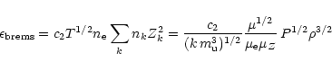
The frequency-integrated volume emissivity for brems- strahlung is
![\begin{figure}
\par\includegraphics[width=8.8cm]{MS10518f1.eps}
\end{figure}](/articles/aa/full/2001/25/aa10518/img77.gif) |
Figure 1: Schematics of the emission region. The region is bounded at the top by the shock front and at the bottom by the white dwarf. |
Figure 1 shows the schematic of an emission region with finite lateral
extent D. The shock is located at ![]()
![]() above the white
dwarf surface. The downstream column density is x = 0 at the shock
and and
above the white
dwarf surface. The downstream column density is x = 0 at the shock
and and ![]()
![]() at the surface of the star, with x and hbeing related by d
at the surface of the star, with x and hbeing related by d![]() dh. The gravity vector
dh. The gravity vector ![]() and
the magnetic field vector
and
the magnetic field vector ![]() are taken parallel to the flow
lines. The radiation-hydrodynamic equations are solved for layers of
infinite D to yield the run of electron temperature and mass
density,
are taken parallel to the flow
lines. The radiation-hydrodynamic equations are solved for layers of
infinite D to yield the run of electron temperature and mass
density,
![]() and
and ![]() .
These profiles are later
employed to calculate the outgoing spectra for emission regions with
finite D by ray tracing, i.e. by adding the contributions from an
appropriate number of rays (Fig. 1 and Sect. 3.1). This
procedure is not self-consistent if optically thick radiative losses
occur from the sides of the column. An appropriate first-order
correction to the temperature structure derived for the infinite layer
is discussed in Sects. 3.2 and 3.3, below.
The treatment of really tall columns requires a different approach
which specifically allows for the emission from the sides of the
column (Wu et al. 1994).
.
These profiles are later
employed to calculate the outgoing spectra for emission regions with
finite D by ray tracing, i.e. by adding the contributions from an
appropriate number of rays (Fig. 1 and Sect. 3.1). This
procedure is not self-consistent if optically thick radiative losses
occur from the sides of the column. An appropriate first-order
correction to the temperature structure derived for the infinite layer
is discussed in Sects. 3.2 and 3.3, below.
The treatment of really tall columns requires a different approach
which specifically allows for the emission from the sides of the
column (Wu et al. 1994).
Radiation intercepted by the white dwarf is either reflected or
absorbed and reemitted by its locally heated atmosphere. We assume
coherent scattering of hard X-rays using the frequency-dependent
reflection albedo ![]() of van Teeseling et al. (1994). The
fraction
of van Teeseling et al. (1994). The
fraction
![]() of the energy is re-emitted in the UV and soft
X-ray regime and is not considered in this paper.
of the energy is re-emitted in the UV and soft
X-ray regime and is not considered in this paper.
Here, we consider simple limiting cases which can, in part, be solved
analytically. Below, we shall discuss our numerical results in terms
of these limiting solutions. The high ![]() ,
low B limit is the
bremsstrahlung-dominated one-fluid solution. In the opposite limit of
low
,
low B limit is the
bremsstrahlung-dominated one-fluid solution. In the opposite limit of
low ![]() ,
high B one enters the non-hydrodynamic regime (Lamb &
Masters 1977). Here, the bombardment solution of a static atmosphere
heated by a stream of fast ions and cooling by cyclotron emission is
an appropriate approximation (Kuijpers & Pringle 1982, WB92, WB93).
,
high B one enters the non-hydrodynamic regime (Lamb &
Masters 1977). Here, the bombardment solution of a static atmosphere
heated by a stream of fast ions and cooling by cyclotron emission is
an appropriate approximation (Kuijpers & Pringle 1982, WB92, WB93).
The one-dimensional, one-fluid hydrodynamic equations with simple
terms for optically thin cooling can be solved analytically (Aizu
1973; Chevalier & Imamura 1982). Integration of Eq. (2) with Eq. (1),
![]() ,
and g = 0 yields
,
and g = 0 yields
![]() which allows to express the
emissivities of Sect. 2.2 as
which allows to express the
emissivities of Sect. 2.2 as
![]() and
and
![]() ,
with f and g being functions of the flow
velocity
,
with f and g being functions of the flow
velocity ![]() and with additional dependencies on the
and with additional dependencies on the ![]() 's
and B contained in the proportionality factors. Integration of the
energy equation over
's
and B contained in the proportionality factors. Integration of the
energy equation over ![]() yields expressions for the column
density
yields expressions for the column
density ![]() and the geometrical shock height
and the geometrical shock height
![]() which reflect the
parameter dependence of
which reflect the
parameter dependence of ![]() ,
,
![\begin{figure}
\par\includegraphics[width=7.2cm,angle=270]{MS10518f2r.eps}
\end{figure}](/articles/aa/full/2001/25/aa10518/img98.gif) |
Figure 2:
Temperature profiles for the ions (dashed
curves) and electrons (solid curves) as functions of column density
x for
|
For a strong shock in a one-fluid plasma with adiabatic index 5/3, the
normalized post-shock velocity
![]()
![]() varies between
1 and 0. The column density x measured from the shock is related to
varies between
1 and 0. The column density x measured from the shock is related to
![]() by (Aizu 1973; Chevalier & Imamura 1982)
by (Aizu 1973; Chevalier & Imamura 1982)
The bombardment solution involves by nature a two-fluid approach. WB92
solved this case using a Fokker-Planck formalism to calculate the
stopping length of the ions and a Feautrier code for the radiative
transfer. WB93 (their Eqs. (8), (9)) provided power law fits to their
numerical results for the column density and the peak electron
temperature. Since the ions are slowed down by collisions with
atmospheric electrons, a factor
![]() appears in
appears in ![]() :
:
With increasing ![]() ,
a shock develops which is initially
cyclotron-dominated and ultimately bremsstrahlung-dominated. Since
,
a shock develops which is initially
cyclotron-dominated and ultimately bremsstrahlung-dominated. Since
![]() reaches
reaches
![]() at some intermediate
at some intermediate ![]() ,
we
expect a smooth transition in peak temperature between these cases.
The situation is quite different for
,
we
expect a smooth transition in peak temperature between these cases.
The situation is quite different for ![]() ,
however. At the
,
however. At the ![]() where
where
![]() equals
equals
![]() ,
,
![]() and
and
![]() differ by more
than two orders of magnitude. The run of
differ by more
than two orders of magnitude. The run of ![]() (
(![]() )
between these
two limiting cases can be determined only with a
radiation-hydrodynamical approach.
)
between these
two limiting cases can be determined only with a
radiation-hydrodynamical approach.
The bombardment solution does not predict the geometrical scale height
of the heated atmosphere which we expect to lie between that of a
corona with an external pressure P = 0 and that of a layer
compressed by the ram pressure ![]()
![]()
![]() 2.
2.
![\begin{figure}
\par\includegraphics[angle=270,width=8.5cm]{MS10518f3r.eps}
\end{figure}](/articles/aa/full/2001/25/aa10518/img119.gif) |
Figure 3:
Normalized electron temperature distributions for
|
In the bombardment solution (Eqs. (17), (18)), the dependence of ![]() and
and
![]() on
on
![]() is obtained from the equilibrium between the
energy gain by accretion,
is obtained from the equilibrium between the
energy gain by accretion,
![]() ,
and the
energy loss by optically thick cyclotron radiation,
,
and the
energy loss by optically thick cyclotron radiation,
![]() ,
where
,
where
![]() is the high-frequency cutoff of the cyclotron spectrum and
is the high-frequency cutoff of the cyclotron spectrum and
![]() the cyclotron frequency. We determine the
limiting harmonic number m* from the cyclotron calculations of
Chanmugam & Langer (1991; their Fig. 5) as
the cyclotron frequency. We determine the
limiting harmonic number m* from the cyclotron calculations of
Chanmugam & Langer (1991; their Fig. 5) as
![]() with
with
![]() and
and
![]() .
This approximation is valid near depth parameters
.
This approximation is valid near depth parameters
![]() and temperatures
and temperatures
![]() and is more adequate for the
cyclotron-dominated emission regions on polars than the frequently
quoted formula of Wada et al. (1980). Replacing
and is more adequate for the
cyclotron-dominated emission regions on polars than the frequently
quoted formula of Wada et al. (1980). Replacing ![]() with
with
![]() in
in
![]() and equating the
accretion and radiative energy fluxes yields the result that a
power of
and equating the
accretion and radiative energy fluxes yields the result that a
power of ![]() is proportional to
is proportional to
![]()
![]() .
The same holds for
.
The same holds for ![]() .
.
We find that the cyclotron-dominated shocks at low ![]() behave
similarly to bombarded atmospheres in that their thermal properties,
too, depend on
behave
similarly to bombarded atmospheres in that their thermal properties,
too, depend on
![]() .
The individual temperature profiles
.
The individual temperature profiles
![]() for different
for different ![]() with the same
with the same
![]() coincide only
in an approximate way, but the dependency on
coincide only
in an approximate way, but the dependency on
![]() holds quite well
for the two characteristic values of each profile,
holds quite well
for the two characteristic values of each profile, ![]() and
and ![]() .
If we
leave the exponent
.
If we
leave the exponent ![]() in
in
![]() as a fit variable,
the smallest scatter in
as a fit variable,
the smallest scatter in ![]() and
and ![]() as functions of
as functions of
![]() is, in fact, obtained for
is, in fact, obtained for
![]() .
.
![\begin{figure}
\par\includegraphics[angle=270,width=8.5cm]{MS10518f4r.eps}
\end{figure}](/articles/aa/full/2001/25/aa10518/img138.gif) |
Figure 4:
Normalized velocity |
Figure 2 shows the temperature profiles ![]() (x) and
(x) and
![]() (x) for
(x) for
![]() = 0.6
= 0.6 ![]() and several
and several ![]() -Bcombinations on a logarithmic depth scale which emphasizes the initial
rise of the profiles. These profiles display a substantial spread in
-Bcombinations on a logarithmic depth scale which emphasizes the initial
rise of the profiles. These profiles display a substantial spread in
![]() and in
and in ![]() ,
reflecting the influence of cyclotron cooling. At
10-2gcm-2s-1, 100MG, cyclotron cooling has reduced
,
reflecting the influence of cyclotron cooling. At
10-2gcm-2s-1, 100MG, cyclotron cooling has reduced ![]() to 6%
and
to 6%
and ![]() to 0.3% of the respective values for the pure bremsstrahlung
solution. We have confidence in our numerical results because they
accurately reproduce the analytic bremsstrahlung solution (see above).
to 0.3% of the respective values for the pure bremsstrahlung
solution. We have confidence in our numerical results because they
accurately reproduce the analytic bremsstrahlung solution (see above).
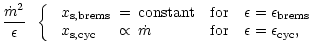
|
|
B |
|
T/ |
||||||||||||||||
| x/ |
10-3 | 0.01 | 0.02 | 0.05 | 0.10 | 0.20 | 0.30 | 0.40 | 0.50 | 0.60 | 0.70 | 0.80 | 0.90 | 0.95 | 0.98 | 0.99 | |||
| 1.000 | 0.999 | 0.995 | 0.989 | 0.973 | 0.945 | 0.886 | 0.821 | 0.751 | 0.674 | 0.589 | 0.494 | 0.382 | 0.245 | 0.156 | 0.085 | 0.054 | |||
| 100 | 10 | 100 | 0.230 | 0.515 | 0.916 | 0.984 | 0.995 | 0.967 | 0.905 | 0.840 | 0.770 | 0.691 | 0.603 | 0.505 | 0.392 | 0.250 | 0.158 | 0.085 | 0.053 |
| 10 | 10 | 10 | 0.230 | 0.515 | 0.915 | 0.984 | 0.996 | 0.968 | 0.906 | 0.842 | 0.770 | 0.692 | 0.604 | 0.506 | 0.393 | 0.250 | 0.159 | 0.082 | 0.048 |
| 1 | 10 | 1 | 0.219 | 0.499 | 0.898 | 0.977 | 0.998 | 0.973 | 0.914 | 0.850 | 0.782 | 0.710 | 0.629 | 0.536 | 0.426 | 0.281 | 0.176 | 0.085 | 0.047 |
| 0.1 | 10 | 0.1 | 0.191 | 0.434 | 0.822 | 0.927 | 0.999 | 0.980 | 0.916 | 0.849 | 0.779 | 0.706 | 0.622 | 0.522 | 0.400 | 0.239 | 0.127 | 0.047 | 0.022 |
| 0.01 | 10 | 0.01 | 0.175 | 0.395 | 0.743 | 0.861 | 0.981 | 0.991 | 0.860 | 0.743 | 0.650 | 0.565 | 0.476 | 0.384 | 0.285 | 0.165 | 0.092 | 0.039 | 0.021 |
| 100 | 30 | 5.75 | 0.228 | 0.512 | 0.914 | 0.984 | 0.994 | 0.966 | 0.903 | 0.836 | 0.766 | 0.686 | 0.598 | 0.499 | 0.388 | 0.247 | 0.153 | 0.080 | 0.046 |
| 10 | 30 | 0.58 | 0.224 | 0.504 | 0.909 | 0.981 | 0.994 | 0.958 | 0.888 | 0.813 | 0.738 | 0.657 | 0.569 | 0.473 | 0.361 | 0.225 | 0.134 | 0.065 | 0.035 |
| 1 | 30 | 0.058 | 0.209 | 0.468 | 0.865 | 0.958 | 0.997 | 0.937 | 0.815 | 0.717 | 0.629 | 0.546 | 0.460 | 0.372 | 0.272 | 0.162 | 0.091 | 0.042 | 0.025 |
| 0.1 | 30 | 0.0058 | 0.185 | 0.408 | 0.738 | 0.849 | 0.971 | 0.997 | 0.833 | 0.657 | 0.548 | 0.468 | 0.401 | 0.336 | 0.274 | 0.197 | 0.145 | 0.085 | 0.045 |
| 0.01 | 30 | 0.00058 | 0.178 | 0.390 | 0.710 | 0.802 | 0.922 | 0.994 | 0.878 | 0.652 | 0.484 | 0.362 | 0.292 | 0.245 | 0.196 | 0.119 | 0.074 | 0.038 | 0.022 |
| 100 | 100 | 0.25 | 0.222 | 0.497 | 0.898 | 0.979 | 0.992 | 0.942 | 0.849 | 0.766 | 0.685 | 0.603 | 0.517 | 0.424 | 0.317 | 0.188 | 0.104 | 0.044 | 0.020 |
| 10 | 100 | 0.025 | 0.206 | 0.468 | 0.839 | 0.940 | 0.999 | 0.927 | 0.756 | 0.639 | 0.541 | 0.450 | 0.367 | 0.289 | 0.201 | 0.103 | 0.043 | 0.011 | 0.006 |
| 1 | 100 | 0.0025 | 0.199 | 0.440 | 0.795 | 0.903 | 0.997 | 0.921 | 0.564 | 0.458 | 0.375 | 0.302 | 0.237 | 0.193 | 0.129 | 0.058 | 0.027 | 0.013 | 0.007 |
| 0.1 | 100 | 0.00025 | 0.180 | 0.354 | 0.626 | 0.727 | 0.880 | 0.976 | 0.966 | 0.600 | 0.131 | 0.097 | 0.084 | 0.077 | 0.063 | 0.047 | 0.038 | 0.030 | 0.022 |
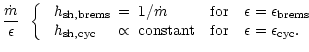
|
| B |
| w = 4v/
|
||||||||||||||||
| x/ | 10-3 | 0.01 | 0.02 | 0.05 | 0.10 | 0.20 | 0.30 | 0.40 | 0.50 | 0.60 | 0.70 | 0.80 | 0.90 | 0.95 | 0.98 | 0.99 | |||
| 1.000 | 0.999 | 0.992 | 0.984 | 0.960 | 0.921 | 0.841 | 0.761 | 0.678 | 0.594 | 0.506 | 0.413 | 0.311 | 0.193 | 0.121 | 0.065 | 0.041 | |||
| 100 | 10 | 100 | 1.000 | 0.999 | 0.992 | 0.985 | 0.961 | 0.920 | 0.840 | 0.760 | 0.676 | 0.593 | 0.504 | 0.411 | 0.310 | 0.191 | 0.119 | 0.064 | 0.039 |
| 10 | 10 | 10 | 1.000 | 0.999 | 0.991 | 0.983 | 0.958 | 0.915 | 0.834 | 0.755 | 0.670 | 0.586 | 0.496 | 0.405 | 0.304 | 0.187 | 0.115 | 0.060 | 0.035 |
| 1 | 10 | 1 | 1.000 | 0.998 | 0.983 | 0.969 | 0.932 | 0.882 | 0.788 | 0.700 | 0.618 | 0.538 | 0.459 | 0.376 | 0.289 | 0.182 | 0.112 | 0.053 | 0.029 |
| 0.1 | 10 | 0.1 | 1.000 | 0.993 | 0.934 | 0.888 | 0.794 | 0.696 | 0.571 | 0.480 | 0.404 | 0.336 | 0.279 | 0.218 | 0.158 | 0.089 | 0.046 | 0.017 | 0.008 |
| 0.01 | 10 | 0.01 | 1.000 | 0.989 | 0.892 | 0.811 | 0.635 | 0.440 | 0.266 | 0.193 | 0.150 | 0.116 | 0.090 | 0.066 | 0.045 | 0.024 | 0.013 | 0.005 | 0.003 |
| 100 | 30 | 5.75 | 1.000 | 0.999 | 0.990 | 0.981 | 0.953 | 0.913 | 0.831 | 0.751 | 0.667 | 0.584 | 0.497 | 0.402 | 0.303 | 0.186 | 0.115 | 0.059 | 0.033 |
| 10 | 30 | 0.58 | 1.000 | 0.996 | 0.972 | 0.948 | 0.902 | 0.947 | 0.758 | 0.676 | 0.597 | 0.517 | 0.437 | 0.352 | 0.264 | 0.159 | 0.094 | 0.044 | 0.022 |
| 1 | 30 | 0.058 | 1.000 | 0.990 | 0.914 | 0.852 | 0.726 | 0.614 | 0.499 | 0.425 | 0.363 | 0.307 | 0.254 | 0.199 | 0.144 | 0.084 | 0.047 | 0.019 | 0.009 |
| 0.1 | 30 | 0.0058 | 1.000 | 0.990 | 0.902 | 0.829 | 0.664 | 0.480 | 0.286 | 0.206 | 0.167 | 0.140 | 0.117 | 0.097 | 0.078 | 0.055 | 0.040 | 0.021 | 0.011 |
| 0.01 | 30 | 0.00058 | 0.999 | 0.982 | 0.895 | 0.824 | 0.653 | 0.435 | 0.148 | 0.087 | 0.062 | 0.045 | 0.036 | 0.029 | 0.023 | 0.013 | 0.008 | 0.004 | 0.003 |
| 100 | 100 | 0.25 | 1.000 | 0.995 | 0.948 | 0.909 | 0.835 | 0.760 | 0.660 | 0.579 | 0.506 | 0.437 | 0.367 | 0.294 | 0.215 | 0.124 | 0.068 | 0.029 | 0.013 |
| 10 | 100 | 0.025 | 1.000 | 0.989 | 0.886 | 0.807 | 0.643 | 0.494 | 0.367 | 0.302 | 0.251 | 0.206 | 0.167 | 0.128 | 0.089 | 0.045 | 0.019 | 0.005 | 0.002 |
| 1 | 100 | 0.0025 | 1.000 | 0.982 | 0.860 | 0.758 | 0.535 | 0.282 | 0.124 | 0.099 | 0.081 | 0.065 | 0.051 | 0.040 | 0.028 | 0.013 | 0.006 | 0.002 | 0.001 |
| 0.1 | 100 | 0.00025 | 0.999 | 0.985 | 0.885 | 0.827 | 0.707 | 0.552 | 0.293 | 0.069 | 0.012 | 0.009 | 0.008 | 0.007 | 0.006 | 0.004 | 0.003 | 0.003 | 0.002 |
Figure 3 displays the normalized profiles of the electron
temperature, ![]() /
/![]() vs. x/
vs. x/![]() ,
for different
,
for different ![]() combinations, covering the range from a bremsstrahlung-dominated flow
with 100gcm-2s-1, 30MG (fat solid curve) to 10-2gcm-2s-1, 100MG
near the non-hydrodynamic limit (dotted curce). They represent an
approximate sequence in
combinations, covering the range from a bremsstrahlung-dominated flow
with 100gcm-2s-1, 30MG (fat solid curve) to 10-2gcm-2s-1, 100MG
near the non-hydrodynamic limit (dotted curce). They represent an
approximate sequence in
![]() ,
but not surprisingly, the shapes
differ somewhat for different
,
but not surprisingly, the shapes
differ somewhat for different ![]() and B combinations
with the same value of
and B combinations
with the same value of
![]() (not shown in Fig. 3).
(not shown in Fig. 3).
Equilibration between electron and ion temperatures is reached at
column densities of ![]() 10
10
![]() gcm-2s-1 depending on
gcm-2s-1 depending on
![]() and B (Fig. 2). At 100gcm-2s-1, 10MG, electrons and ions
equilibrate as early as
and B (Fig. 2). At 100gcm-2s-1, 10MG, electrons and ions
equilibrate as early as ![]()
![]() ,
while at 10-2gcm-2s-1,
100MG, equilibration length and
,
while at 10-2gcm-2s-1,
100MG, equilibration length and ![]() are of the same order,
indicating the approach to the non-hydrodynamic regime. A peculiar
feature of the latter profile is the extended low-temperature tail
which was not adequately resolved by WB96. This tail appears when
equilibration occurs near the temperature at which cyclotron cooling
becomes ineffective and the density is sufficiently high for
bremsstrahlung to take over. It is hydrodynamic in origin. Apart from
the tail, the temperature profile at 10-2gcm-2s-1, 100MG is very
close to that obtained by the non-hydrodynamic approach of WB92,
WB93. The low-temperature tail is responsible for a low-temperature
thermal emission component with
are of the same order,
indicating the approach to the non-hydrodynamic regime. A peculiar
feature of the latter profile is the extended low-temperature tail
which was not adequately resolved by WB96. This tail appears when
equilibration occurs near the temperature at which cyclotron cooling
becomes ineffective and the density is sufficiently high for
bremsstrahlung to take over. It is hydrodynamic in origin. Apart from
the tail, the temperature profile at 10-2gcm-2s-1, 100MG is very
close to that obtained by the non-hydrodynamic approach of WB92,
WB93. The low-temperature tail is responsible for a low-temperature
thermal emission component with
![]() keV.
keV.
The initial rise of the individual temperature profiles is similar and
is very rapid following approximately ![]()
![]() (Fig.2). One half of
(Fig.2). One half of ![]() is reached at 0.001
is reached at 0.001![]() in
the bremsstrahlung-dominated case and at 0.006
in
the bremsstrahlung-dominated case and at 0.006![]() near the
non-hydrodynamic limit. Further downstream the profiles differ
substantially. In the bremsstrahlung-dominated case, the peak electron
temperature is reached quickly, while in the cyclotron-dominated flow
it occurs at the same x at which half of the accretion energy has
been radiated away. The reason is that a temperature gradient is
needed to drive about one half of the radiative flux across the shock
front, while the other half enters the white dwarf atmosphere. In
the plane-parallel geometry, the optically thick radiative transfer
requires the electron temperature at the shock front to stay below the
peak electron temperature :
near the
non-hydrodynamic limit. Further downstream the profiles differ
substantially. In the bremsstrahlung-dominated case, the peak electron
temperature is reached quickly, while in the cyclotron-dominated flow
it occurs at the same x at which half of the accretion energy has
been radiated away. The reason is that a temperature gradient is
needed to drive about one half of the radiative flux across the shock
front, while the other half enters the white dwarf atmosphere. In
the plane-parallel geometry, the optically thick radiative transfer
requires the electron temperature at the shock front to stay below the
peak electron temperature :
![]() .
This is why we opted to start the
integration with the initial values
.
This is why we opted to start the
integration with the initial values
![]() = 0 and
= 0 and
![]() as given by
Eq.(7). Because of the rapid initial rise in T(x), our
results would have been practically the same had we set
as given by
Eq.(7). Because of the rapid initial rise in T(x), our
results would have been practically the same had we set
![]() =
0.5
=
0.5![]() .
.
To facilitate the modeling of specific geometries, we provide the
normalized temperature and density profiles for a sequence of ![]() combinations in Table 1. We also provide best fits to
combinations in Table 1. We also provide best fits to ![]() /
/
![]() and
and ![]() as functions of
as functions of
![]() .
.
![\begin{figure}
\par\includegraphics[angle=270,width=8.7cm]{MS10518f5r.eps}
\par\end{figure}](/articles/aa/full/2001/25/aa10518/img150.gif) |
Figure 5:
Maximum electron temperature |
![\begin{figure}
\par\includegraphics[angle=270,width=8.8cm]{MS10518f6r.eps}
\end{figure}](/articles/aa/full/2001/25/aa10518/img151.gif) |
Figure 6:
Column density |
![\begin{figure}
\par\includegraphics[angle=270,width=8.8cm]{MS10518f7r.eps}
\end{figure}](/articles/aa/full/2001/25/aa10518/img152.gif) |
Figure 7:
Same as Fig. 6 but for geometrical
shock height
|
For calculations of the bremsstrahlung emission, we need the profiles
of the mass density which varies as
![]() .
Figure 4 shows the normalized velocity profiles for
.
Figure 4 shows the normalized velocity profiles for
![]() =
0.6
=
0.6 ![]() and the same
and the same ![]() combinations as in
Fig. 3. In the limit of pure bremsstrahlung cooling, the
velocity profile is indistinguishable from that given by the inversion
of Eq. (12). Increased cyclotron cooling causes a similar
depression at intermediate x as seen in the temperature
profiles. Table 1 (bottom) provides the velocity profiles in numerical
form for the same parameters as above.
combinations as in
Fig. 3. In the limit of pure bremsstrahlung cooling, the
velocity profile is indistinguishable from that given by the inversion
of Eq. (12). Increased cyclotron cooling causes a similar
depression at intermediate x as seen in the temperature
profiles. Table 1 (bottom) provides the velocity profiles in numerical
form for the same parameters as above.
In what follows, each model is represented by one "data point''.
Figure 5 shows ![]() /
/
![]() vs.
vs.
![]() for
for
![]() =0.6
=0.6 ![]() and
B = 10-100MG. The dependence of
and
B = 10-100MG. The dependence of ![]() on
on
![]() is equally well
documented for
is equally well
documented for
![]() =0.8 and 1.0
=0.8 and 1.0 ![]() ,
but for clarity we do not
show these data. The 0.6
,
but for clarity we do not
show these data. The 0.6 ![]() results can be fitted by
results can be fitted by
| M | a0 | a1 | b0 | c0 | |||
| ( |
(s) | (108cm) | |||||
| 0.6 | 0.91 | 0.968 | 1.67 | 6.5 | 0.70 | 0.95 | 1.0 |
| 0.8 | 0.86 | 0.954 | 1.54 | 7.5 | 0.54 | 1.30 | 0.7 |
| 1.0 | 0.90 | 0.934 | 1.25 | 8.0 | 0.45 | 1.75 | 0.5 |
The transition of ![]() between the bombardment and the bremsstrahlung
solutions (Eqs. (17) and (13)) is more complicated
than that of
between the bombardment and the bremsstrahlung
solutions (Eqs. (17) and (13)) is more complicated
than that of ![]() .
Figure 6 shows
.
Figure 6 shows ![]() as a function of
as a function of
![]() for
for
![]() = 0.6
= 0.6 ![]() and
B = 10 - 100MG. Again, the data points for
0.8 and 1.0
and
B = 10 - 100MG. Again, the data points for
0.8 and 1.0 ![]() are not shown for clarity. We fit
are not shown for clarity. We fit ![]() by
by
![\begin{figure}
\par\includegraphics[angle=270,width=8.8cm]{MS10518f9r.eps}
\end{figure}](/articles/aa/full/2001/25/aa10518/img167.gif) |
Figure 9:
Cyclotron section of the spectral energy
distributions for the same set of parameters as in Fig. 8, except
|
Figure 7 shows the quantity
![]() B72.6 for
B72.6 for
![]() =
0.6
=
0.6 ![]() and for field strengths between 10 and 100MG. We fit
the data by
and for field strengths between 10 and 100MG. We fit
the data by
Copyright ESO 2001
![\begin{displaymath}x=c_1\upsilon_{\rm o}^2\left[\sqrt{3}{-}\frac{\pi}{3}{-}\frac...
...2}
{+}{\rm cos}^{-1}\left(1{-}\frac{\omega }{2}\right)\right].
\end{displaymath}](/articles/aa/full/2001/25/aa10518/img101.gif)
![\begin{figure}
\par\includegraphics[angle=270,width=8.8cm]{MS10518f8r.eps}
\end{figure}](/articles/aa/full/2001/25/aa10518/img155.gif)
![\begin{displaymath}\frac{1}{T_{\rm max}} = \left[\left(\frac{1}{a_0\,T_{\rm
max,...
...c{1}{a_1\,T_{\rm
max,brems}}\right)^\alpha ~\right]^{1/\alpha}
\end{displaymath}](/articles/aa/full/2001/25/aa10518/img158.gif)
![\begin{displaymath}\frac{1}{x_{\rm s}} = \left[\left(\frac{\mu}{b_0\,\mu_{\rm e}...
... \left(\frac{1}{x_{\rm
s,brems}}\right)^\beta\right]^{1/\beta}
\end{displaymath}](/articles/aa/full/2001/25/aa10518/img164.gif)
![\begin{displaymath}\frac{1}{h_{\rm sh}B_7^{2.6}} = \left[\left(\frac{\mu}{c_0\,\...
..._7^{-2.6}}{h_{\rm sh,brems}}\right)
^\gamma~\right]^{1/\gamma}
\end{displaymath}](/articles/aa/full/2001/25/aa10518/img169.gif)