The Sedov (1959) model does not give a centrally-concentrated morphology due to geometrical properties of self-similar solutions. The solutions are 1-D and give a specific internal profile of the flow gas density: most of the mass is concentrated near the shock front. These factors and cumulation of the emission along the line of sight cause a shell-like morphology. If we consider a more complicated nonuniform ISM, we get beyond one dimension and need to consider additional parameters responsible for nonuniformity of the medium and orientation of a 3-D object.
Projection effects may essentially change the morphology of SNRs (Hnatyk & Petruk 1999). Densities over the surface of a nonspherical SNR may essentially differ in various regions. If the ambient density distribution provides a high density in one of the regions across the shell of SNR and is high enough to exceed the internal column density near the edge of the projection, we will see a centrally-filled projection of a really shell-like SNR. Such density distribution may be ensured e.g. by a molecular cloud located near the object.
What is a really shell-like 3-D SNR? We suggest that such a remnant has internal density profiles similar to those in the Sedov (1959) solutions. Thus, we separate a shell-like SNR (as an intrinsic property of a 3-D object) from its limb brightened projection (as a morphological property of the projection). Let us call shell-like SNRs with centrally-filled projections "projected composites''.
For simplicity, let us consider the case of a 2-D SNR
and the characteristics
of SNR and the surrounding medium which could be possible
on smoothed boundaries of
molecular clouds. Thus, SNR evolves in the ambient medium with
hydrogen number density n distributed according to
| Parameter | Model | |||||
| a | b | c | d | e | f | |
|
|
2.5 | 2.5 | 2.5 | 5 | 10 | 40 |
|
|
1.0 | 6.8 | 17.7 | 6.8 | 6.8 | 6.8 |
|
|
8 | 7 | 6.5 | 7 | 7 | 7 |
|
|
9.5 | 94 | 280 | 98 | 95 | 94 |
|
|
1.4 | 1.8 | 2.1 | 1.4 | 1.2 | 1.1 |
|
|
1.9 | 2.8 | 3.1 | 1.9 | 1.5 | 1.1 |
|
|
3.5 | 7.9 | 9.8 | 3.7 | 2.2 | 1.2 |
|
|
9.5 | 45 | 84 | 11 | 3.9 | 1.4 |
|
|
34.1 | 36.7 | 37.3 | 36.4 | 36.2 | 36.1 |
|
|
0.98 | 3.2 | 3.1 | 3.9 | 4.1 | 4.2 |
|
|
0.43 | 2.1 | 2.3 | 0.72 | -0.10 | -0.54 |
|
|
1.6 | 1.8 | 3.6 | 1.3 | 1.2 | 1.3 |
Gas density n and temperature T distributions inside the volume of a nonspherical SNR are obtained with the method of Hnatyk & Petruk (1999).
The equilibrium thermal X-ray emissivities are taken from Raymond & Smith (1977).
We make simple estimations of the radio morphology of SNR in a nonuniform medium as described below, on the basis of a model for synchrotron emission from SNRs developed by Reynolds (1998, hereafter R98) and Reynolds & Chevalier (1981).
The volume emissivity in the radio band at some frequency ![]() is
is
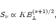 |
(2) |
The ambient field is assumed to be uniform
(polarization observations
support the assumption that the magnetic fields
in molecular clouds may be ordered over large scales,
e.g. Goodman et al. 1990;
Messinger et al. 1997;
Matthews & Wilson 2000 and others).
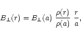
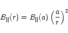
Component
![]() is not modified by the shock:
is not modified by the shock:
![]() (indices "s" and "o" refer to the values at the shock and to the
surrounding medium, respectively).
Component
(indices "s" and "o" refer to the values at the shock and to the
surrounding medium, respectively).
Component ![]() rises everywhere at the shock by the factor of
rises everywhere at the shock by the factor of
![]() .
No further turbulent amplification of the magnetic field is assumed.
Components
.
No further turbulent amplification of the magnetic field is assumed.
Components
![]() and
and ![]() evolve differently behind the
shock front (R98; Reynolds & Chevalier 1981).
Since the magnetic field is flux-frozen,
evolve differently behind the
shock front (R98; Reynolds & Chevalier 1981).
Since the magnetic field is flux-frozen,
![]() ,
the tangential component in each 1-D sector of the remnant is
,
the tangential component in each 1-D sector of the remnant is
 |
(3) |
 |
(4) |
In each fluid element, energy density ![]() of relativistic
particles is proportional to the energy density of the magnetic field
of relativistic
particles is proportional to the energy density of the magnetic field
 |
(5) |
Each individual electron loses its energy due to the adiabatic expansion:
 |
(7) |
Figures 1a,b demonstrate the influence of the projection on a
thermal X-ray morphology of SNR. The X-ray brightness maximum
located near the shock
front in the shell-like projection (
![]() )
moves towards
the centre of the projection with the increase of
)
moves towards
the centre of the projection with the increase of ![]() from
from
![]() to
to
![]() .
For clarity we only consider here the most emphatic limit case
.
For clarity we only consider here the most emphatic limit case
![]() .
Radio images (Figs. 1c,d)
show that the radio limb-brightened morphology
clearly appears at
.
Radio images (Figs. 1c,d)
show that the radio limb-brightened morphology
clearly appears at
![]() ,
i.e. if both the density
gradient and the magnetic field are nearly aligned.
,
i.e. if both the density
gradient and the magnetic field are nearly aligned.
Variation of the magnetic field orientation changes the
radio morphology from shell-like to barrel-like
(Kesteven & Caswell 1987; Gaensler 1998).
Contrast
![]() in the radio surface brightness decreases with increasing
in the radio surface brightness decreases with increasing
![]() ,
from 2.7 (
,
from 2.7 (
![]() )
to 1.8 (
)
to 1.8 (
![]() ).
Such behaviour of the radio morphology
may be used for testing orientation of the
magnetic field.
).
Such behaviour of the radio morphology
may be used for testing orientation of the
magnetic field.
Thus, we found that the morphological properties of the projected composites match the basic features of the TXC class: centrally-peaked distribution of the thermal X-ray surface brightness is within the area of the radio shell; emission arises from the swept-up ISM material.
Let us consider physical properties of TXCs.
a) The column number density increases from the edge towards
the centre of the projection (e.g., for model b from
![]() to
to
![]() ).
b) The diffuse optical nebulosity over the
internal region of the projection may naturally take place in such a
model. c) Emission measure
).
b) The diffuse optical nebulosity over the
internal region of the projection may naturally take place in such a
model. c) Emission measure
![]() (
(![]() is the electron number density,
l is the length within SNR)
is the highest in the X-ray peak
because both
is the electron number density,
l is the length within SNR)
is the highest in the X-ray peak
because both ![]() and l are maximum there
(Fig. 2).
and l are maximum there
(Fig. 2).
As Fig. 3 demonstrates, the distribution of X-ray surface
brightness has strong maximum ![]() around the centre and
a weaker shell with second maximum
around the centre and
a weaker shell with second maximum
![]() just behind the
forward shock.
It is essential that such a morphology takes place in different X-ray bands
(lines b, 1, 2).
The contrasts
just behind the
forward shock.
It is essential that such a morphology takes place in different X-ray bands
(lines b, 1, 2).
The contrasts
![]() in X-ray surface brightness
depend on the photon energy band and may lie
within a wide range: in our models from 3 to 200
for
in X-ray surface brightness
depend on the photon energy band and may lie
within a wide range: in our models from 3 to 200
for
![]() (Table 1).
The ratios of X-ray luminosity
(Table 1).
The ratios of X-ray luminosity
![]() of central region
of central region
![]() to the luminosity
beyond
to the luminosity
beyond
![]() are 0.16, 5.2 and 16 in models
a, b and c, respectively.
Thus, observational property d of TXCs takes place
just at the adiabatic stage.
are 0.16, 5.2 and 16 in models
a, b and c, respectively.
Thus, observational property d of TXCs takes place
just at the adiabatic stage.
![\begin{figure}
\par\includegraphics[width=8.8cm,clip]{h24562.eps}
\end{figure}](/articles/aa/full/2001/19/aah2456/img128.gif) |
Figure 3:
a and b. Evolution of the distribution of thermal X-ray
surface brightness a) and spectral index b).
Solid curves are labelled with the model codes according to
Table 1; they represent |
Surface distribution of spectral index
![]()
![]() ,
of the thermal X-ray emission
where
,
of the thermal X-ray emission
where ![]() is the continuum emissivity
and
is the continuum emissivity
and
![]() is the photon energy,
gives us profiles of
effective temperature T of the column of emitting gas
(
is the photon energy,
gives us profiles of
effective temperature T of the column of emitting gas
(
![]() ,
if the Gaunt factor is assumed to be constant).
Figure 3 shows that the temperature may either increase or decrease towards the
centre. Decreasing takes place early in the adiabatic phase.
Variation of the spectral index lies within factors 1.6 to 3.6
at the adiabatic stage (Table 1); the contrast
in the spectral index distribution increases with age. Such
values correspond to the possible range of temperature variation
over the projection of thermal X-ray composites.
,
if the Gaunt factor is assumed to be constant).
Figure 3 shows that the temperature may either increase or decrease towards the
centre. Decreasing takes place early in the adiabatic phase.
Variation of the spectral index lies within factors 1.6 to 3.6
at the adiabatic stage (Table 1); the contrast
in the spectral index distribution increases with age. Such
values correspond to the possible range of temperature variation
over the projection of thermal X-ray composites.
In order to reveal the dependence of the distributions of S and ![]() on the ISM density gradient,
a number of models with different h were calculated (Fig. 4
and Table 1).
The surface brightness distribution has a stronger peak for a stronger gradient.
With increasing h, the outer shell becomes more prominent in the projection.
Only a scale-height of order
on the ISM density gradient,
a number of models with different h were calculated (Fig. 4
and Table 1).
The surface brightness distribution has a stronger peak for a stronger gradient.
With increasing h, the outer shell becomes more prominent in the projection.
Only a scale-height of order
![]() can cause projected
composites. A less strong gradient of the ambient density makes
effective temperature T
more uniformly distributed in the internal part of the projection.
can cause projected
composites. A less strong gradient of the ambient density makes
effective temperature T
more uniformly distributed in the internal part of the projection.
Copyright ESO 2001
![\begin{figure}
\par\includegraphics[width=8.8cm,clip]{h24561.eps}
\end{figure}](/articles/aa/full/2001/19/aah2456/img105.gif)

![\begin{figure}
\par\includegraphics[width=8.8cm,clip]{h2456add.eps}
\end{figure}](/articles/aa/full/2001/19/aah2456/img118.gif)