1 - Departament d'Astronomia i Meteorologia, Universitat de Barcelona, Martí i Franquès 1, 08028 Barcelona, Spain
2 - Institut d'Estudis Espacials de Catalunya, Edifici Nexus, Gran Capità 2-4, 08034 Barcelona, Spain

Abstract
We have developed a detailed standard chemical evolution model to study the evolution of all the chemical elements up to the iron peak in the solar vicinity. We consider that the Galaxy was formed through two episodes of exponentially decreasing infall, out of extragalactic gas. In a first infall episode, with a duration of $\sim$ 1 Gyr, the halo and the thick disk were assembled out of primordial gas, while the thin disk formed in a second episode of infall of slightly enriched extragalactic gas, with much longer timescale. The model nicely reproduces the main observational constraints of the solar neighborhood, and the calculated elemental abundances at the time of the solar birth are in excellent agreement with the solar abundances. By the inclusion of metallicity-dependent yields for the whole range of stellar masses we follow the evolution of 76 isotopes of all the chemical elements between hydrogen and zinc. Those results are compared with a large and recent body of observational data, and we discuss in detail the implications for stellar nucleosynthesis.

Key words: nuclear reactions, nucleosynthesis, abundances - stars: abundances - Galaxy: abundances - Galaxy: evolution - Galaxy: general

The chemical evolution of our Galaxy has been extensively studied in the last years. During the last decade a great deal of new data have become available, revealing in principle the chemical history of the Milky Way and building up a set of observational constraints that have to be fulfilled by any successful theoretical model. These observational results concern in particular the age-metallicity relation (Meussinger et al. 1991; Edvardsson et al. 1993; Rocha-Pinto et al. 2000), star metallicity distribution (Wyse & Gilmore 1995; Rocha-Pinto & Maciel 1996; Jørgensen 2000), abundance ratios of an increasing number of chemical elements, both in halo and local disk stars (Sneden et al. 1994; McWilliam et al. 1995; Ryan et al. 1996; Chen et al. 2000, among others), and radial abundance gradients (see Henry & Worthey 1999 for a review).

These observational efforts have been accompanied by the publication of several theoretical models which try to interpret the data. Most of those works are standard open chemical evolution models (Carigi 1994; Giovanoli & Tosi 1995; Prantzos & Aubert 1995; Timmes et al. 1995 (hereafter TWW1995); Chiappini et al. 1997, 1999; Thomas et al. 1998; Chang et al. 1999; Goswami & Prantzos 2000 (hereafter GP2000), etc.) in which the Galaxy is assembled by infall of extragalactic gas and that use different prescriptions for the main ingredients, i.e. infall rate and composition of the accreted material, initial mass function (IMF), star formation rate (SFR) and stellar yields. Chemodynamical models have also been published (Steinmetz & Müller 1994; Samland et al. 1997; Samland 1998; Berczik 1999), but due to the numerical complexity they have to introduce several approximations in the treatment of stellar lifetimes and yields.

As pointed out by GP2000, while the prescriptions for the IMF, the SFR and the infall rate are just empirical recipes due to our poor understanding of the physical processes involved, the stellar yields can be determined from first principles, as they rely upon the much better known theory of stellar evolution. However, there still remain severe uncertainties in the stellar yields, especially for massive stars where the treatment of convection, the inclusion or neglect of mass loss, the explosion mechanisms, etc. could give rise to large discrepancies in the final yields of several elements.

Most of the available models use metallicity-independent yields and/or concentrate on a limited number of chemical species. TWW1995 were the first to consider the evolution of the complete ensemble of light and intermediate-mass elements (from H to Zn) by including in a simple infall model for the galactic disk the yields of massive stars with metallicities between Z=0 and $Z=Z _{\odot }$ of Woosley & Weaver (1995), and adopting for the CNO yields of low and intermediate mass stars the Renzini & Voli (1981) results. Recently, GP2000 have reanalyzed the evolution of the elements from C to Zn by means of an infall model that treats separately the halo and the disk, but they only take into account stellar yields from massive stars, assuming zero net yields for intermediate mass stars.

In this paper we present new calculations of the evolution in the solar neighborhood of all the chemical elements up to Zn, in the framework of a two-infall model (Chiappini et al. 1997) for the formation of the Galaxy, with metallicity-dependent stellar yields for the whole range of stellar masses considered. Also, we include the contributions from nova nucleosynthesis, since significant amounts of several isotopes (mainly ⁷Li, ¹³C, ¹⁵N, and ¹⁷O) could be produced by nova outbursts. The plan of the paper is as follows: in Sect. 2 we present and discuss the main ingredients of our model: infall assumptions, SFR, IMF and nucleosynthetic prescriptions. Inspired by the recent observations of Wakker et al. (1999), who have reported the detection of a massive cloud with a metallicity $\sim$ 0.09 times solar falling into the galactic disk, we adopt as our standard model one in which first the halo and the thick disk of the Milky Way form by accretion of primordial gas, and then, in a second infall episode lasting up to present, the thin disk assembles from slightly enriched extragalactic material; however, we have also considered a popular standard model with infall of primordial gas along the whole galactic evolution. In Sect. 3 we compare our results with the main observational constraints in the local disk (G-dwarf distribution, age-metallicity relation, solar abundances, supernova rates, etc.). The core of the paper is presented in Sect. 4, where we compare in detail the evolution of the different elements studied with the available observational data, including the most recent observations. Finally, in Sect. 5 we give the main conclusions of our work.

2 The chemical evolution model

We have developed a standard open chemical evolution model where the Milky Way builds up gradually by infall of primordial and, lately, slightly enriched gas. No outflows are considered. The disk is divided into concentric independent rings 1 kpc wide, and we neglect any radial flow between them. Inside each zone we assume instantaneous mixing so that the stellar ejecta are completely mixed with the interstellar medium as soon as the stars die; in this way, each ring is made of an homogeneous mixture of gas, stars and stellar remnants, and the local interstellar medium is characterized at any time by a unique composition; therefore, the quantities describing the state of each zone, i.e. surface density of total, gas and stellar masses, chemical abundances, etc., are functions only of galactocentric radius and time. We relaxed the instantaneous recycling approximation by treating in detail the delay in chemical enrichment due to the finite stellar lifetimes, which we adopt from the work of the Geneva group (Schaller et al. 1992; Charbonnel et al. 1996).

The model solves numerically the classical set of nonlinear-integro differential equations of galactic chemical evolution (Tinsley 1980; Pagel 1997). In the solar ring we follow the evolution of 76 isotopes from hydrogen to zinc. For simplicity we use, as in TWW1995, Gaussian quadrature summation for the mass integrals (Press et al. 1992), and a Cash-Karp stepper method (Press & Teukolsky 1992) for the explicit time integrations. In the following subsections we discuss the main ingredients of the model.

2.1 Infall

Closed box models of galactic evolution face the so-called "G-dwarf problem'', the formation of too many long lived stars at low metallicities. The most common way out of this problem is to turn to open models which consider that the Galaxy forms by continuous infall of extragalactic material. In fact, there are observational indications of current infall onto the Galactic disk from external regions in the form of High Velocity Clouds moving towards the Galactic disk, as first suggested by Larson (1972). Although the interpretation of such clouds as gas of extragalactic origin has been a matter of debate, the observation of both High (Mirabel 1981) and Very High Velocity Clouds (Mirabel & Morras 1984) seemed to confirm the idea of current infall with rates of the order of 1 $M _{\odot }$ yr^-1. Recently, Wakker et al. (1999) have reported the detection of a massive ( $\sim$ 10⁷ $M _{\odot }$ ) cloud falling into the disk of the Milky Way, with a metallicity 0.09 times solar, and the authors give strong arguments for the extragalactic origin of the cloud.

Different types of infall have been explored in several models, but not all of them can solve the G-dwarf problem. For instance, constant infall rates just balancing star formation produce too many stars at high metallicity. Most of the "successful'' models use simple exponentially decreasing infall rates (TWW1995; Prantzos & Aubert 1995; Thomas et al. 1998) for the assembling of the galactic disk, with timescales of the order of 3-4 Gyr at the solar ring, but recent determinations of the metallicity distribution of disk stars by Wyse & Gilmore (1995) and Rocha-Pinto & Maciel (1996) require, to be reproduced by the models, longer timescales, with typical values of 7 Gyr at solar galactocentric distances (Chiappini et al. 1997; Prantzos & Silk 1998; Boissier & Prantzos 1999). It is worth mentioning that some chemodynamical models also infer long timescales for the formation of the disk (Samland et al. 1997).

Recently Chiappini et al. (1997), and lately Chang et al. (1999), have included implicitly the halo phase evolution through models that assume two subsequent infall episodes. In the first episode the halo and the thick galactic disk form in a very short time ( $\tau _{\rm T}\leq$ 1 Gyr). At the end of this phase, the thin disk begins to form in a second infall episode characterized by much longer timescales. In this way, the material that eventually forms the disk has an extragalactic origin.

In the present work, following Chiappini et al. (1997), we adopt the two-infall exponentially decreasing model. Therefore, the time evolution of the total surface mass density in the solar ring is given by

The coefficients $A(r_{\odot })$ and $B(r_{\odot })$ are fixed by imposing that the current total surface mass densities of the thick and thin disks in the solar neighborhood are well reproduced by the model

Based on the observations of Wakker et al. (1999), we begin accreting primordial material during the halo-thick disk phase, and then, when the thin disk initiates its formation, we assume that the infalling material has already being slightly enriched, with a typical metallicity of $0.1~Z _{\odot }$ in solar proportions. By comparison, we have also calculated models that only accrete primordial matter during the whole evolution. Even if there are not substantial differences between the results we obtain in both types of models, in agreement with Tosi (1988) who showed that as long as the metallicity of the accreted material remains below 0.1 $Z _{\odot }$ there are little changes in the model results, we obtain slightly better agreement with the observational constraints in the solar region for the model that incorporates enriched infall during the assembling of the thin disk.

2.2 Star formation rate

In view of the difficulties in understanding the rather complicated process of star formation, standard models for the chemical evolution of the Galaxy adopt different analytical prescriptions for the star formation rate (SFR) in terms of intrinsic parameters of spiral galaxies. The simplest and still commonly used law for star formation is the Schmidt (1959) law: $\Psi \propto \sigma ^{k}_{\rm g}$ , proportional to some power (between 1 and 2) of the surface gas density. Observations by Kennicutt (1998) of the correlation between average SFR and surface gas densities (total: atomic plus molecular) in spiral and starburst galaxies point to a value of the exponent in the Schmidt law of $k \sim 1.5$ . Besides this global behaviour, the SFR has also to show dependence on the local environment, which in turn is typically a function of galactocentric distance.

The precise radial dependence of the SFR varies according to the scenario considered for star formation. In theories that describe star formation as a local self-regulating process through the balance between the gravitational settling of the gas onto the disk, that enhances star formation, and the energy injected back into the interstellar medium by massive young stars under the form of winds and supernova explosions, which heat and expand the gas reducing the process of star formation (Talbot & Arnett 1975), the SFR is a function of the local gravitational potential and, therefore, of the total surface mass density, $\sigma$ . In the original Talbot & Arnett (1975) formulation, $\Psi \propto \sigma ^{k-1}\sigma ^{k}_{\rm g}$ . We notice that some chemodynamical models (Burkert et al. 1992) find a similar dependence of the SFR on the total surface mass density.

Observational support for such star formation law has been obtained by Dopita & Ryder (1994), who showed the existence in spiral disks of an empirical link between H $_{\alpha }$ emission, tracing current star formation, and the I-band surface brightness, a measure of the contribution of the old stellar component and, therefore, of the total surface mass density. This observed relation is well fitted by a SFR law very similar to that of Talbot & Arnett (1975): $\Psi \propto \sigma ^{n}\sigma _{\rm g}^{m}$ , with n=1/3and m=5/3. Moreover, self-regulated star formation can accommodate the observed correlation between surface brightness and oxygen abundance in late spiral disks (Edmunds & Pagel 1984; Ryder 1995).

2.3 Initial mass function

The initial mass function (IMF) constitutes another basic input in models of chemical evolution, since it determines in which proportions stars of different masses enter into play; that, in turn, fixes the averaged stellar yields and remnant masses for each generation of stars.

In general, the assumed form of the IMF is a declining function of mass in terms of a power law: $\Phi (M)\propto M^{-x}$ , constant in space and time. Salpeter's (1955) version, with x=1.35 for the whole mass range has been commonly used. However, recent studies reviewed by Scalo (1998), Kroupa (1998) and Meyer et al. (2000) indicate, within still rather large uncertainties, that observations are consistent with an IMF almost flat at low masses, how flat still being a matter of debate (for instance, Reid & Gizis 1997 find a unique slope of x=0.05 for $0.1 \leq M/M_{\odot }\leq 1$ , but Kroupa 1998 claims that such slope is only appropriate for $M/M _{\odot } \leq 0.5$ ), and declining as a power law with a slope similar to the Salpeter's one above 1 $M _{\odot }$ , although there are again discrepancies on the actual value of x. For instance, Massey et al. (1995) find slopes $x \sim$ 1-1.5 in OB associations, while for massive field stars Massey (1998) obtains very steep IMFs, with values of $x \sim$ 3-4.

Another aspect of the IMF that has not yet been satisfactorily settled, neither observationally nor theoretically, is its time behavior. There seems to be a tendency among observational researchers to favor no variations of the IMF, although in a recent review Scalo (1998) argues against its universality in space and time. Besides, an IMF producing more massive stars in the early Galaxy has been invoked as a solution to the G-dwarf problem. Nevertheless, in a recent paper, Chiappini et al. (2000) have investigated the effects on galactic chemical evolution of several time dependent IMFs and conclude that the combination of infall and a constant IMF is still the best choice to reproduce the observational constraints in the Milky Way.

In this paper we adopt the constant IMF version of Kroupa et al. (1993), which consists in a three slope power law. In the range of very low masses the slope is quite flat, x = 0.3 for $M < 0.5~M _{\odot }$ , it steepens to x = 1.2 in the interval $0.5~M_{\odot} \leq~ M \leq 1 ~M_{\odot}$ , and in the high mass regime $M > 1~M _{\odot }$ the slope agrees with the one by Scalo (1986) x = 1.7. As usual, we normalize to unity this IMF between a minimum stellar mass of 0.08 $M _{\odot }$ , the H-burning limit, and a maximum of 100 $M _{\odot }$ .

2.4 Nucleosynthesis prescriptions

The chemical yields synthesized by stars in different stellar mass ranges are a key ingredient when trying to understand the chemical evolution of galaxies, in particular those corresponding to "massive stars'', stars that end their lives in Type II supernova explosions, since they are the main responsibles for the enrichment of the Universe in intermediate and heavy nuclei, through both hydrostatic burning (elements up to calcium) and explosive nucleosynthesis (iron peak elements, to which Type Ia supernovae are also important contributors). Even if the uncertainties in the theory of stellar evolution are far lesser than those affecting the SFR or the IMF, there still remain serious discrepancies in the literature about the treatment of crucial aspects of stellar evolution. For instance, presupernova configurations are affected by the precise formulation of convection, semi-convection and overshooting, the adopted nuclear reaction rates (especially for the ¹²C( $\alpha ,\gamma$ ) ¹⁶O reaction), the inclusion or not of mass loss and rotation, etc. A similar situation holds for the results of core collapse supernova explosions. In fact, in current calculations the explosion itself is induced rather arbitrarily and the explosion energy is fixed by imposing a given value for the final kinetic energy. Also, the ejected mass crucially depends on the degree of "fall-back'', and thus on the precise details of the explosion. We thus see that the published stellar yields are yet plagued with severe uncertainties.

Although the evolution during the thin disk epoch will be hardly affected by the slight metallicity dependence shown in the published stellar yields, the early halo-thick disk phase could be strongly influenced by the material ejected by stars of different metallicities. Hence, we will consider metallicity dependent yields for the whole stellar mass range.

2.4.1 Massive stars: 8 ${\mathsfsl {M _{\odot }}\leq {\mathsfsl M} \leq 100~ {\mathsfsl M _{\odot }}}$

We assume that stars in this mass interval end their lifes as core collapse supernovae. The two major sources in this mass range, widely used in chemical evolution models, are Woosley & Weaver (1995) (hereafter WW1995), who calculated full stellar models without mass loss nor rotation, for stars with masses comprised between 12 $M _{\odot }$ and 40 $M _{\odot }$ and with different initial metallicities ( $Z/Z _{\odot } =0$ , 10^-4, 10^-2, 10^-1 and 1), and Thielemann et al. (1996), who calculated the evolution of He cores corresponding to stars of solar initial metallicity with masses up to 70 $M _{\odot }$ . There are noticeable differences between the WW1995 results for Z=0 and $Z \neq 0$ , while the yields and stellar remnant masses for nonzero initial metallicities give more similar results. Solar composition models of WW1995 and Thielemann et al. (1996) give almost the same values for the yields of the CNO isotopes, but non-negligible differences exist for other important elements. For instance, the magnesium yield is systematically lower in WW1995 as a consequence of the different treatments of convection. In the case of the iron yield, WW1995 give much higher values than Thielemann et al. (1996) for stars with masses below $\sim$ 35 $M _{\odot }$ , since it is very sensitive to the mass cut that separates the ejecta and the material that falls back onto the compact remnant which, as mentioned above, depends in turn on the detailed explosion mechanism (see Thomas et al. 1998, and Chiappini et al. 1999 for a complete discussion).

Lately, Limongi et al. (2000), from full stellar models, again without mass loss nor rotation, have also presented yields for massive stars in the range 13-25 $M _{\odot }$ , for three metallicities (Z=0, 10^-3, and 0.02). As shown by GP2000, the main difference with respect to WW1995 is a more marked odd-even effect in the case of Limongi et al. (2000) yields, which translates into systematically lower yields of odd Z elements.

In this paper we adopt the metallicity-dependent yields of WW1995 for massive stars between 8 and 100 $M _{\odot }$ . The reasons for this choice are twofold: they are the results of full evolutionary calculations and they consider a wider interval of masses and metallicities as compared with the work of Limongi et al. (2000). In particular, we take their models A up to 25 $M _{\odot }$ , and their models B for 30, 35 and 40 $M _{\odot }$ (the explosion energy in models B is higher than in models A). Those yields have been extrapolated up to 100 $M _{\odot }$ , even though this has just a minor effect on the final results since the Kroupa et al. (1993) IMF produces very few stars more massive than 40 $M _{\odot }$ .

TWW1995 suggested that a better agreement with most of the observed evolution of the abundances is obtained if the WW1995 iron yields are reduced by a factor of two. Observational estimates of the iron synthesized in SN 1987A (the explosion of a 20 $M _{\odot }$ belonging to a stellar system, LMC, with an estimated $Z \sim 0.1~Z _{\odot }$ ) and of SN 1993J (whose progenitor was a 14 $M _{\odot }$ star in the galaxy M81, where $Z \sim Z _{\odot }$ ) also points to such an overestimate (Thomas et al 1998). Therefore, in view of the uncertainties arising from the flaws in the explosion calculations, we reduce by a factor of 2 the nominal yields of WW1995.

2.4.2 Low and intermediate mass stars: ${\mathsfsl {M\leq}}~8~{\mathsfsl M _{\odot}}$

As is well known, single stars in this mass range pollute the interstellar medium through moderate stellar winds and planetary nebula ejection, ending their lives as white dwarfs. These stars make important contributions to the He, C and N galactic contents. Here again important uncertainties on the final yields exist that result from the treatment of mass loss, convection, evolution on the asymptotic giant branch, etc.

The yields of Renzini & Voli (1981) have been extensively used in chemical evolution models. However, in the last years several groups have published new evolutionary calculations for stars belonging to this mass interval and for different initial metallicities (Marigo et al. 1996; van den Hoek & Groenewegen 1997). In this work the contribution to the galactic enrichment by these stars has been taken from van den Hoek & Groenewegen (1997), who give yields for stars with masses comprised between 0.9 and 8 $M _{\odot }$ and consider five initial metallicities, since the work of Marigo et al. (1996) is limited to stars with $M \leq 4~M _{\odot}$ , besides taking into account convective overshooting, which is not considered in WW1995.

2.4.3 Type Ia supernovae

There is a general agreement that Type Ia supernovae are important contributors to iron and other iron peak elements (in particular ⁵⁸Ni and ⁵⁴Cr) in the late disk evolution, up to the point that they could be responsible for up to $\sim$ 2/3 of the total iron contents (TWW1995). We adopt the conventional view that Type Ia supernovae are carbon deflagration of massive C-O white dwarfs in binary systems. The contribution of Type Ia supernovae to the chemical enrichment of the galaxy, especially the iron content, has been calculated following the prescriptions of Matteucci & Greggio (1986), where Type Ia supernovae come from binary systems with a minimum mass of 3 $M _{\odot }$ , in order to ensure that the accreting white dwarf eventually reaches the Chandrasekhar mass, and a maximum mass of 16 $M _{\odot }$ , if we assume that C-O white dwarfs come from primaries up to 8 $M _{\odot }$ . Thus, the amount of isotope i due to this source is given by

2.4.4 Classical novae

Although classical novae have little or no influence on the evolution of the abundances of most of the chemical elements included in our calculations, according to José & Hernanz (1998) they can be significant contributors to certain isotopes that are strongly overproduced in nova explosions relative to the solar system abundances (in particular those with overproduction factors larger than 1000). ⁷Li, ¹³C, ¹⁵N and ¹⁷O are some of the isotopes whose abundances could be affected by novae.

In order to obtain the nova rates we assume that novae take place in binary systems made of a white dwarf coming from stars with main sequence masses in the interval $M_{1}^{m} = 1~M _{\odot }$ to $M_{1}^{M} = 8~ M _{\odot }$ , while the secondary stars have masses between $M_{2}^{m} = 0.5 ~M _{\odot }$ and $M_{2}^{M} = 1.5~ M _{\odot }$ . The rate of those explosions can be estimated by a procedure similar to that used by Matteucci & Greggio (1986) to calculate the rate of SN Ia:

The yields for the classical nova outburst are an average of those given by José & Hernanz (1998). We have considered that 30% of the nova outbursts come from ONe white dwarf progenitors, while 70% come from CO ones.

3 Model results versus observational constraints

As we have discussed in the previous section, there are large uncertainties in the ingredients of standard chemical evolution models which translate into a series of more or less free parameters, e.g. infall timescales, efficiency and exponent of the SFR, slope of the IMF, etc. Fortunately, for the solar neighborhood, the number of observational constraints is large enough to restrict the space of variation of these parameters (Boissier & Prantzos 1999). Results for the whole galactic disk will be the subject of another paper.

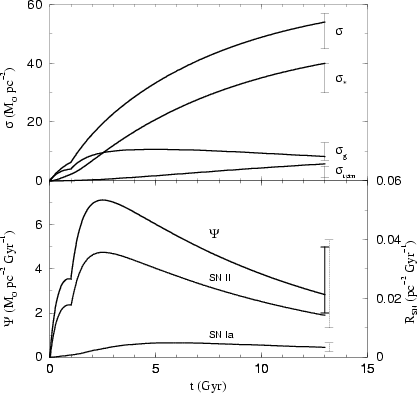
3.1 Surface densities, SFR and supernova rates

First of all, any successful model has to reproduce the present-day surface density of total mass, gas, star and stellar remnants, the current rate of star formation, infall and supernovae (both Type Ia and Type II). In Table 1 we show our results for the present values ( $t _{\rm G} = 13$ Gyr) of those quantities compared with the current observational values for the solar vicinity. The time evolution of the surface densities of total mass ( $\sigma$ ), stars ( $\sigma _{\star }$ ), gas ( $\sigma _{\rm g}$ ), and stellar remnants ( $\sigma _{\rm rem}$ ) are displayed in the upper panel of Fig. 1, while in the lower panel appear the star formation rate, and the Type II and Type Ia supernova rates. We see from Table 1 and Fig. 1 that the model presented in the previous section nicely fits the observations.

Table 1: Calculated and observed present values for several relevant quantities in the solar ring
model Obser. Ref.

$\sigma _{g}$ ( $M _{\odot }$ pc^-2) 8.27 7-13 1

$\sigma _{\star }$ ( $M _{\odot }$ pc^-2) 39.93 30-40 2

$\sigma _{\rm rem}$ ( $M _{\odot }$ pc^-2) 5.77 2-4 3

$\sigma _{g}/\sigma _{\rm tot}$ 0.15 0.05-0.2

$\sigma _{\rm inf}$ ( $M _{\odot }$ pc^-2 Gyr^-1) 1.38 0.3-1.5 4

$\Psi$ ( $M _{\odot }$ pc^-2 Gyr^-1) 2.84 2-5 5

SN Ia per century 0.41 0.17-0.7 6

SN II per century 1.76 0.55-2 6

SN II/SN Ia 4.3 3-6 6

Novae (yr^-1) 40.0 20-60 7

**Table 1:** Calculated and observed present values for several relevant quantities in the solar ring
	model	Obser.	Ref.
$\sigma _{g}$ ( $M _{\odot }$ pc^-2)	8.27	7-13	1
$\sigma _{\star }$ ( $M _{\odot }$ pc^-2)	39.93	30-40	2
$\sigma _{\rm rem}$ ( $M _{\odot }$ pc^-2)	5.77	2-4	3
$\sigma _{g}/\sigma _{\rm tot}$	0.15	0.05-0.2
$\sigma _{\rm inf}$ ( $M _{\odot }$ pc^-2 Gyr^-1)	1.38	0.3-1.5	4
$\Psi$ ( $M _{\odot }$ pc^-2 Gyr^-1)	2.84	2-5	5
SN Ia per century	0.41	0.17-0.7	6
SN II per century	1.76	0.55-2	6
SN II/SN Ia	4.3	3-6	6
Novae (yr^-1)	40.0	20-60	7

References.-(1) Dickey (1993); Flynn et al. (1999); (2) Gilmore et al. (1989); (3) Méra et al. (1998); (4) Portinari et al. (1998) and references therein; (5) Güsten & Mezger (1982); (6) Tamman et al. (1994); (7) Hatano et al. (1997).

$\begin{figure} \resizebox*{\hsize}{!}{\includegraphics{MS10620f1.eps}}\par\end{figure}$	Figure 1: Upper panel: time evolution of the surface densities of total mass ( $\sigma \protect$ ), visible stars ( $\sigma _{\star }\protect$ ), gas ( $\sigma _{\rm g}\protect$ ), and stellar remnants ( $\sigma _{\rm rem}\protect$ ) for our two-infall model. Lower panel: evolution of the stellar formation rate, as well as the Type II and Type Ia supernova rates
Open with DEXTER

3.2 Age-metallicity relation

Our model also fulfills the requisite of producing an age-metallicity relation in agreement with the observed one. The age-metallicity relation (AMR) shows the evolution of the ratio [Fe/H], taken as a measure of the metallicity of the Galaxy, as a function of time. The pioneering work by Twarog (1980) showed that [Fe/H] rises steeply during the first 2 Gyr up to a value of $\sim$ -0.5 dex, and afterwards increases smoothly with time towards the solar value, although the data presented a large dispersion, and age-bins and average metallicity per bin were used. Later reexamination of Twarog's data by Meussinger et al. (1991) found a similar AMR. More recently, Edvardsson et al. (1993), based on a different sample of nearby F and G stars, obtained for binned data a good agreement with previous results, but they claimed that the large dispersion found in their unbinned data was essentially real and not observational (but see Garnett & Kobulnicky 2000). Finally, Rocha-Pinto et al. (2000) obtained a chromospheric AMR using a sample of 552 late-type dwarfs that basically confirms the observed trends, but with almost half the scatter found by Edvardsson et al. (1993).

Models of chemical evolution that adopt the instantaneous mixing approximation, like ours, cannot produce any dispersion at all, and at most they can only fit the mean relation. Therefore, the AMR is a less tight constraint than the previous one, even though the average relation must be fitted by successful models.

We present in the lower panel of Fig. 2 our results for the evolution with time of [Fe/H] compared with the AMR from Meussinger et al. (1991), Edvardsson et al. (1993), and with the more recent data from Rocha-Pinto et al. (2000). Just for completeness, in the upper panel we also show the evolution of the total metallicity in terms of the solar value. Again our model fits well the averaged trend of the data, although, as stated above, this is not a really tight constraint, because almost any model can produce a reasonable AMR.

$\begin{figure} \resizebox*{8.8cm}{!}{\includegraphics{MS10620f2.eps}}\par\end{figure}$	Figure 2: Upper panel: evolution with time of the total metallicity Z normalized to the solar value $Z _{\odot }$ . Lower panel: time evolution of the ratio [Fe/H] for contributions from Type II supernovae (thin line) and for Type II plus Type Ia supernovae (thick line)
Open with DEXTER

Nearly 2/3 of the present total iron contents are made by Type Ia supernovae, the other third coming from Type II supernovae. We remind here that the iron yields for Type II supernovae used in this work are half those of WW1995 in order to obtain a better fit to the evolution of the element abundances. That is also indicated by iron abundance measurements in supernova ejecta. In any case, as pointed out by TWW1995, whatever contribution to the present galactic iron contents from Type II supernovae comprised between one and two thirds is allowed by our current understanding of stellar physics.

3.3 G-dwarf distribution

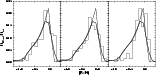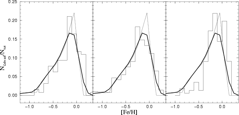
$\begin{figure} \resizebox*{18cm}{!}{\includegraphics{MS10620f3.eps}}\end{figure}$	Figure 3: Rough (thin dashed curve) G-dwarf metallicity distributions and Gaussian convolved distribution (thick solid curve) compared with observational data by Wyse & Gilmore (1995) (left panel), Rocha-Pinto & Maciel (1996) (central panel) and by Jørgensen (2000) (right panel)
Open with DEXTER

The stars of spectral type G have main-sequence lifetimes comparable or even larger than the estimated age of the Galaxy. Hence, the distribution in metallicity of a complete sample of these stars in the solar neighborhood carries memory of the star formation history. This makes the observed G-dwarf distribution one of the more stringent constraints for models of galactic chemical evolution.

As is well known, the paucity of G-dwarf stars at low metallicities, referred to as the "G-dwarf problem'', cannot be explained by simple, closed box models. Several solutions have been proposed to solve this problem, but open models with progressive infall of primordial or slightly enriched material with long timescales for the disk formation, like ours, are still the best option (Chiappini et al. 1997), besides of being compatible with dynamical simulations of the formation of galactic disks (Burkert et al. 1992), and with the observation of infall of High and Very High Velocity Clouds.

Figure 3 compares the predicted G-dwarf distribution produced by our model with the most recent observational data from Wyse & Gilmore (1995) (left panel), Rocha-Pinto & Maciel (1996) (central panel) and Jørgensen (2000) (right panel). The direct results are displayed by thin dashed lines, while the thick solid ones show the convolution with a Gaussian with a dispersion of 0.15 in order to simulate observational and intrinsic scatter. Very good agreement is reached, especially for the rising part of the distribution and the location and height of the peak when comparing with the two first sets of data. In the case of the distribution from Jørgensen (2000), the fit is still reasonable, the peak is again well reproduced, but the model shows a low metallicity tail (around [Fe/H] $\sim$ -0.5) that is higher than the data. The comparison between theoretical results and observations could be improved by relaxing the instantaneous mixing approximation, introducing thus in the models the intrinsic scatter. Our results confirm once more that infall models with long timescales for the assembling of the disk are capable of solving the G-dwarf problem.

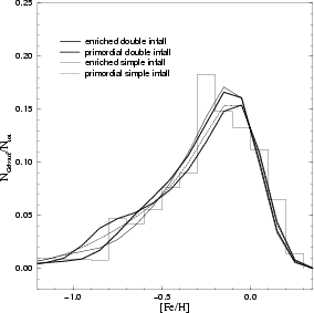
$\begin{figure} \resizebox*{\hsize}{!}{\includegraphics{MS10620f4.eps}}\end{figure}$	Figure 4: G-dwarf distributions obtained for different types of infall. The observational data correspond to Rocha-Pinto & Maciel (1996)
Open with DEXTER

As indicated above, our model uses a double exponential infall in order to treat as separate entities the halo-thick disk and the thin disk, and we consider accretion of enriched material ( $Z=0.1~Z _{\odot }$ ) during the thin disk phase. We have also calculated models that incorporate primordial material both in the halo-thick disk and in the thin disk phases, as well as models that only consider simple exponential infall of primordial and primordial plus enriched material which, if not appropriate for the halo and thick disk, are relevant when making comparisons for the thin disk properties. In all those models we have adopted the same timescale for the galactic disk, i.e., 7 Gyr. We obtain in all cases very similar results for the final characteristics of the solar ring, but slight differences appear for the convolved G-dwarf distributions, which are displayed in Fig. 4, where for clarity only the observations by Rocha-Pinto & Maciel (1996) are shown. One and two infall models with the same composition of the incorporated matter are almost indistinguishable, but primordial composition models show a moderate excess of stars in the low metallicity tail and lower maxima than those obtained in enriched models.

3.4 Solar abundances

$\begin{figure} \resizebox*{17.7cm}{!}{\includegraphics{MS10620f5.eps}}\end{figure}$

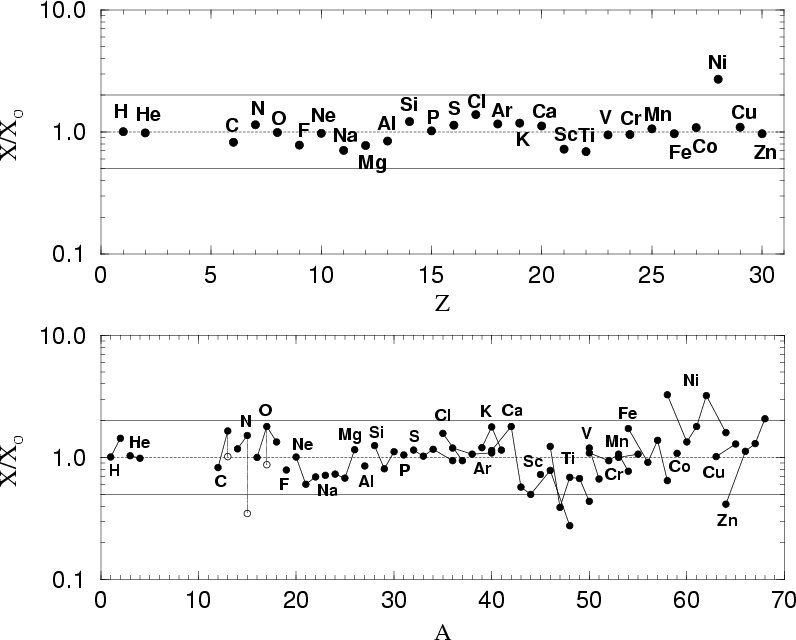
Figure 5: Mass fractions of the calculated elements (upper panel), from hydrogen to zinc (lithium, beryllium and boron are not shown), and of all their stables isotopes (lower panel) in the interstellar gas at the time of solar birth, relative to the solar abundances of Anders & Grevesse (1989). The isotopes of the same element are connected by solid lines. The dashed horizontal line would correspond to a perfect agreement, while the two solid lines correspond to a discrepancy by a factor of 2. We take as successful those elements and isotopes whose calculated abundances fall within this factor of 2 of their solar values. The three open circles in the lower panel represent the relative abundances of ¹³C, ¹⁵N and ¹⁷O when nova yields are excluded from the calculations

Open with DEXTER

We present in Fig. 5 the calculated mass fractions of the elements (upper panel) and all their stable isotopes (lower panel) studied in this work (except LiBeB isotopes, whose abundances have important contributions from galactic cosmic ray nucleosynthesis, not included in the present calculations) in the interstellar gas at the time of the solar birth, 4.5 Gyr ago, compared with the observed solar values (Anders & Grevesse 1989), considered as representative of the composition of the interstellar gas at that epoch. We must remind here that this last assumption is far from being definitely settled, since measured abundances in regions of recent star formation, like the Orion nebula, show metallicities lower than solar (see, for instance, Cardelli & Federmann 1997). Due to the uncertainties existing in the observational values, we consider as good agreement abundances within a factor of 2 of their solar value. As it can be seen in Fig. 5, all the elemental abundances fulfill this criterion, nickel excepted, which is clearly oversolar, and the model makes the correct solar metallicity. The isotopic abundances are also nicely adjusted. The spread for isotopes below calcium is lower than above it, reflecting the uncertainties in the present modeling of Type II supernova explosions.

The production factors for hydrogen, helium and the most important CNO isotopes are nearly equal to unity. In particular, the solar ³He abundance is almost exactly reproduced by our models without taking into account any partial destruction by extra-mixing on the RGB (see, however, Romano et al. 2000). The inclusion of novae worsens our results for ¹³C and ¹⁷O, which are then a little bit overabundant. On its turn, ¹⁵N is a factor of 3 below its solar value when only nucleosynthesis in massive stars is considered, and contribution from novae is mandatory to render its abundance compatible with the solar value.

A few isotopes fall out of the acceptable range. ⁴⁸Ca, ⁴⁷Ti, ⁵⁰Ti and ⁶⁴Zn are underproduced (especially ⁴⁸Ca). In the case of the neutron-rich isotopes ⁴⁸Ca and ⁵⁰Ti there could be a substantial contribution from Type Ia supernovae resulting from initially slow deflagrations at high density (Woosley & Eastman 1994). ⁴⁷Ti (and, in lesser extent, ⁴⁴Ca and ⁵¹V) have been traditionally problematic; these isotopes could have noticeable contributions from sub-Chandrasekhar explosions of SNeIa (Shigeyama et al. 1992; Woosley & Weaver 1994). Additional contributions to the abundance of ⁶⁴Zn could be obtained, as pointed out by TWW1995, from weak s-process in massive stars or classical s-process in low-mass AGB stars.

On the other hand, there is a small overproduction of nickel, due to the large yields of ⁵⁸Ni in the adopted model for SNeIa and the high production of ⁶²Ni in current models of massive star explosions, which reflects the inaccuracies involved in current supernova modeling.

As noted in previous works (TWW1995; GP2000), the fact that the solar abundances of all isotopes up to the iron peak, that cover a range of almost 9 orders of magnitude, are so precisely reproduced by current models of chemical evolution indicates that the present understanding of stellar nucleosynthesis is basically correct, at least to first order.

4 Abundance ratios evolution

We have calculated the evolution in time of all the stable isotopes of thirty chemical elements from H to Zn with the nucleosynthetic prescriptions detailed above. Our results are displayed in Figs. 6 to 15, where we compare the predicted ratios [X/Fe] as functions of [Fe/H] with observational data of spectroscopic abundances in nearby stars. Data sources are detailed in the legends of the figures. As the data normally refer to elemental abundances, for each element we sum over the calculated isotopic abundances.

We note that following the suggestion of TWW1995 we have reduced the iron yields of WW1995 by a factor of 2. The reduced iron yields, well within the current inaccuracies in supernova models, not only give a better agreement with the observed elemental abundances but they are also consistent with the amount of iron ejected in recently observed Type II supernovae .

We consider that the calculated abundance evolution is only significant for [Fe/H] $\geq -$ 3, a value that our model reaches at $t \sim$ 30 Myr, which approximately corresponds to the lifetime of a 8-9 $M _{\odot }$ star. This means that only after reaching such global metallicity the yields of massive stars are fully averaged over the IMF, therefore reducing the possible uncertainties in the yields of individual stars.

4.1 The CNO elements

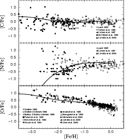
We present in Fig. 6 the results obtained in our calculations for the evolution of CNO elemental abundances with respect to iron.

Carbon and iron are primary elements but have different production sites: carbon is made by the triple- $\alpha$ process in hydrostatic helium burning in massive and, mostly, in intermediate and low-mass stars, while Fe is produced by explosive burning in Type II and Type Ia supernovae. Observations of carbon abundances in halo and disk dwarfs (field giants are not reliable indicators of ab initio carbon abundance due to the effects of the first dredge-up) do actually show that [C/Fe] is almost constant in time, with a value approximately solar (Laird 1985; Tomkin et al. 1986; Carbon et al. 1987; McWilliam et al. 1995), although there is an important dispersion in the data at all metallicities. Those surveys also seem to indicate some trend towards slightly higher values of [C/Fe] at low [Fe/H], as confirmed to first order by Wheeler et al. (1989) after reanalyzing the data available at that epoch, although observational uncertainties counsel to take with some caution this upturn at low metallicity.

$\begin{figure} \resizebox*{\hsize}{!}{\includegraphics{MS10620f6.eps}}\end{figure}$	Figure 6: Evolution of abundances ratios [X/Fe] as a function of [Fe/H] for the CNO elements. Upper panel: carbon; central panel: nitrogen; lower panel: oxygen
Open with DEXTER

Our results show that the synthesis of carbon and iron by massive stars suffices to explain the observations in halo stars. The [C/Fe] ratio shows a slow decline towards the solar value during the halo-thick disk epoch, which indicates that intermediate-mass stars, whose lifetimes permit them to evolve during the late halo phase, do not give very important contributions to the carbon contents. The bump around [Fe/H] $\sim -$ 1, at the beginning of the thin disk phase, results from the contribution of intermediate and, especially, low-mass stars ( $M < 2~M _{\odot }$ ), which eject important amounts of carbon but no iron. But the iron ejected by Type Ia supernovae, which start to contribute around the same epoch, compensates and finally overwhelms the role of the low mass stars.

The synthesis of ¹³C in intermediate and low-mass stars is capable of building up the solar contents. The inclusion of novae produces a small overabundance of ¹³C at the time of the solar birth.

The evolution of the ratio [N/Fe] as a function of [Fe/H] is displayed in the second graph of Fig. 6. The three observational surveys shown in the figure present a large scatter and there are no observations below [Fe/H] $\sim -$ 2.5. The data seem to indicate that [N/Fe] remains more or less constant over the range of metallicities studied, but besides the large dispersion, there are also uncertainties on the value of the constant, although the data are compatible with a solar value. Our model predicts a rapid increase of [N/Fe] at low metallicity, which shows that metal poor massive stars do not produce primary nitrogen. The ratio [N/Fe] steadily increases up to [Fe/H] $\sim -1$ due to the progressive contribution of mostly secondary nitrogen ejected by intermediate and low-mass stars, until the iron production by Type Ia supernovae compensates the ejecta of intermediate stars, flattening the evolution of [N/Fe].

TWW1995 obtained primary nitrogen production by metal poor massive stars with masses above 30 $M _{\odot }$ by considering enhanced convective overshooting, but still within the theoretical uncertainties, due to the violent effects of the penetration of the helium convective burning shell into the hydrogen shell, although this effect does not occur in more metal-rich massive stars. This could be a promising mechanism to explain the abundance pattern of damped Lyman- $\alpha$ systems (Matteucci et al. 1997). Synthesis of primary nitrogen due to the injection of protons into helium burning zones could also happen in stellar models that include rotation (Heger et al. 1999; Maeder & Meynet 2000). Massive stars produce some ¹⁵N but the dominant contribution in our model comes from novae.

Oxygen is exclusively produced by massive stars and dominates their ejecta. Until recent years the observational status of the oxygen abundance in dwarfs and G and K giants showed a nearly constant value of [O/Fe] $\sim$ 0.5 for [Fe/H] $\leq -$ 1, and a gradual decline in the disk. In fact, this is the canonical behavior of the so-called $\alpha$ -elements (O, Mg, Si, S, Ca, Ti): almost flat evolution in the halo, and a gradual decline in the disk due to the iron production by Type Ia supernovae. However, recent data by Israelian et al. (1988) and Boesgaard et al. (1999), which agree with earlier results from Abia & Rebolo (1989), are in contradiction with the idea of an oxygen plateau, since they find that [O/Fe] increases between [Fe/H] = -1 and -3, from 0.6 to 1, which means a slope in this range of $- 0.31 \pm 0.11$ .

Our calculations show that [O/Fe] begins with a value of the order of 1 at very low metallicity, and it slowly declines during the thick disk phase, in part because massive stars of different masses and initial metal contents produce different O/Fe ratios, and also because Type Ia supernovae begin to inject iron already in the halo-thick disk phase, though their influence is stronger during the thin disk epoch, when Type Ia supernovae reach their highest rate, as it is clearly shown by the steeper decline of [O/Fe] for [Fe/H] $\geq -$ 1. This behaviour is in agreement with previous results by TWW1995 and Chiappini et al. (1997). We obtain a slope of -0.28, which clearly indicates a deviation from the traditional oxygen plateau, although a little bit less pronounced than in the new data. We will see the same kind of evolution, although less marked, for the rest of the $\alpha$ -elements.

$\begin{figure} \par\resizebox*{\hsize}{!}{\includegraphics{MS10620f7.eps}}\end{figure}$	Figure 7: Upper panel: evolution of the ratio [F/Fe] as a function of [Fe/H]. Lower panel: evolution of the ratio [F/O] as a function of [Fe/H], compared with observational points from Jorissen et al. (1992)
Open with DEXTER

4.2 Fluorine

In our calculations fluorine is synthesized (together with ⁷Li and ¹¹B which will not be treated here) by the so-called neutrino-induced nucleosynthesis in Type II supernova explosions. The amount of fluorine produced by neutrino spallation of ²⁰Ne is extremely sensitive to the neutrino fluxes and spectra used in the explosion calculations, which render its yield very uncertain.

The upper panel of Fig. 7 displays the evolution versus iron abundance of the ratio [F/Fe]. Our model predicts a practically constant and almost solar [F/Fe]. In the lower panel of Fig. 7 we present the ratio [F/O] compared to the only available set of observations in the literature. In agreement with TWW1995, our model predicts strong subsolar [F/O] ratios at low metallicity, which is a result of the early efficient oxygen enrichment by massive stars and not of a deficient production of fluorine, while it fits the observed abundances of normal K giants.

Most of the plotted data correspond to spectroscopically peculiar giant stars whose abundances are affected by stellar evolution, although the high ratios observed in those stars also point to contributions other than from massive stars. Forestini & Charbonnel (1997) suggest fluorine production in the helium burning shell of AGB stars, and Meynet & Arnould (2000) contributions from WR stars. A reliable history of fluorine will only be settled when we gain new insight into the contributions from different kinds of stars.

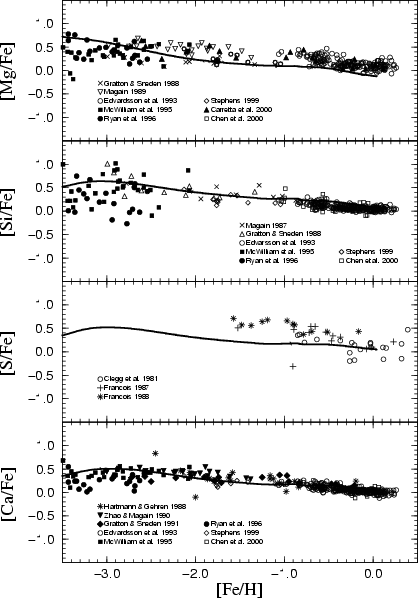
4.3 The $\alpha \protect$ -elements magnesium, silicon, sulphur and calcium

Our results for the evolution of the ratios [ $\alpha$ /Fe] for magnesium, silicon, sulphur and calcium, plotted in Fig. 8, closely follow the general trends of the data. Chiappini et al. (1999) pointed out that the so-called "plateau'' for the $\alpha$ -elements at low metallicities is not perfectly flat, but instead presents a slight slope. In fact, that is exactly what we find: the abundance ratios slowly increase with decreasing [Fe/H], in good agreement with the work of McWilliam et al. (1995) and that of Ryan et al. (1996) for magnesium, silicon and calcium, although the slopes are shallower than for oxygen.

$\begin{figure} \par\resizebox*{\hsize}{!}{\includegraphics{MS10620f8.eps}}\end{figure}$	Figure 8: Evolution of the abundance ratios to iron of the $\alpha \protect$ elements Mg, Si, S, and Ca as a function of [Fe/H]
Open with DEXTER

The results for silicon and calcium are in excellent agreement with the data. The evolution of magnesium and sulphur, however, is less satisfactory.

In the case of magnesium, though we begin with typical halo values, the rapid decline of [Mg/Fe] gives values a little lower than observed in the thick disk phase, but still marginally compatible with the observations. Later on, when the thin disk starts, the iron from Type Ia supernovae worsens the problem and we clearly underestimate the [Mg/Fe] ratio in the disk. In principle, the metallicity-independent yields for massive stars from Thielemann et al. (1996) or the WW1995 yields for solar metallicity could solve this discrepancy (Thomas et al. 1998; Chiappini et al. 1999), but this type of yields are not appropriate when studying the galactic halo. Since the magnesium yields of WW1995 increase with the stellar mass, the use of the rather steep IMF of Kroupa et al. (1993) worsen the situation. As pointed out by GP2000, the use of the metallicity dependent yields of Limongi et al. (2000) will probably solve the underproduction of magnesium but the ratios $\alpha$ /Mg will not reproduce the observations. The fact that current yields from massive stars cannot completely explain the magnesium evolution could indicate the need for a supplementary source of this element, either in low and intermediate mass stars or by enhancing the magnesium yield in Type Ia supernovae (TWW1995).

The paucity of data for sulphur at low [Fe/H] does not allow precise comparisons, but if the points by François (1987, 1988) around and below [Fe/H] $\sim -$ 1 adequately represent the main trend, a supplementary production of sulphur at low metallicity seems necessary. Given our nucleosynthetic sources, sulphur is only produced by massive stars, and the uncertainties in the WW1995 yields of metal poor massive stars could be the cause of the low [S/Fe] at low [Fe/H]. It has been suggested, however, that the [S/Fe] values measured in the halo stars should be reduced by 0.2 dex (Lambert 1989). If that were the case, our results for sulphur would nicely fit the corrected data.

4.3.1 The magnesium isotopes

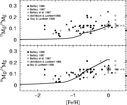
Unlike most of the chemical elements, in the case of magnesium the evolution of the isotopic ratios can be compared with observational results.

$\begin{figure} \par\resizebox*{\hsize}{!}{\includegraphics{MS10620f9.eps}}\end{figure}$	Figure 9: Evolution of the magnesium isotopic ratios ²⁵Mg/ ²⁴Mg (upper panel) and ²⁶Mg/ ²⁴Mg (lower panel) as a function of metallicity
Open with DEXTER

In the upper panel of Fig. 9 we show our results for the evolution of the ratio ²⁵Mg/ ²⁴Mg as a function of [Fe/H], while in the lower panel appears the evolution of the ratio ²⁶Mg/ ²⁴Mg. The three isotopes are produced during the hydrostatic evolution of massive stars. Since in the WW1995 yields for massive stars ²⁴Mg is basically a primary isotope, while the neutron-rich isotopes ²⁵Mg and ²⁶Mg increase with metallicity (both are affected by the neutron excess), it is to be expected, indeed, that both ratios decrease towards lower metallicities.

Our results, similar to those found by TWW1995 and by GP2000, follow the expected trend, but the model produces isotopic ratios clearly below the observations in the halo-thick disk phase (i.e., [Fe/H] $\leq -$ 1). If the WW1995 yields do not underestimate the magnesium isotopic yields, a supplementary source of ²⁵Mg and ²⁶Mg is needed, for instance through s-process in AGB stars (Iben & Renzini 1983).

In the thin disk phase ([Fe/H] -1), the model reproduces well the global trend of the observations, with both ratios systematically increasing with metallicity. The ratio ²⁵Mg/ ²⁴Mg reaches the solar value. However, the ²⁶Mg/ ²⁴Mg ratio at [Fe/H] = 0 is $\sim$ 50% higher than solar, again in agreement with the results of GP2000 who attribute the overabundance of ²⁶Mg at the solar birth to the effects of the IMF of Kroupa et al. (1993) that favor the production of ²⁶Mg in front of that of ²⁴Mg.

4.4 Sodium, aluminum and potassium

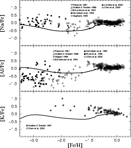
Sodium, aluminum and potassium are odd elements (besides, sodium and aluminum are monoisotopic) mainly produced by massive stars. They are subjected to the odd-even effect, i.e., stellar yields increasing with metallicity. Therefore, their galactic abundance ratios to iron must increase with time, although the evolution of the ratio [element/Fe] could be affected by the iron production by Type Ia supernovae, especially in the disk. One can eliminate the effects of Type Ia supernovae on the abundance evolution of odd elements by plotting the ratio [element/Mg], as in TWW1995, because magnesium is also nearly exclusively synthesized in massive stars, or by using as metallicity indicator an element more reliable than iron, which is affected by uncertainties such as the evolution of Type Ia supernova rates or the mass cut and explosion energy in Type II supernovae, as done by GP2000 who use calcium instead of iron as metallicity indicator.

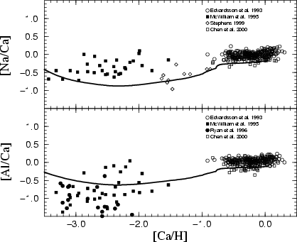
We display in Fig. 10 the calculated [Na/Fe] (upper panel) and [Al/Fe] (central panel). In Fig. 11 we also show the ratios [Na/Ca] and [Al/Ca] using [Ca/H] as a measure of the metallicity. It is worth stressing that the evolution of the calcium abundance obtained in our model agrees very well with the data (see Fig. 8).

$\begin{figure} \resizebox*{\hsize}{!}{\includegraphics{MS10620f10.eps}}\end{figure}$	Figure 10: Evolution of Na, Al and K abundance ratios to iron in terms of [Fe/H] as metallicity indicator
Open with DEXTER

The observed sodium to iron ratios display a plateau in the disk. The situation for the halo stars is less clear. The rather old data by Peterson (1981) indicate a rapid decrease from [Fe/H] = -1 to [Fe/H] =-2. Recent observations by Stephens (1999) show the same trend, but most other observations point to a constant [Na/Fe] $\sim$ 0, although with large dispersion. We obtain an almost constant, but lower than the data, abundance up to [Fe/H] $\sim -$ 2.5, and a steep increase at the beginning of the thin disk formation that ends in a plateau lower than observed.

The calculated evolution of [Al/Fe] begins almost flat and is clearly higher than the data from halo stars. Later, it slowly increases at the thick-thin disk transition, but, as with Na, remains below the disk star observations.

The abundance ratio to calcium of both elements shows now the odd-even effect (see Fig. 11). We still have low [Na/Ca] in the complete range of [Ca/H], but the aluminum ratio shows a better agreement with the observations. We remind that our models underproduce the solar sodium by a factor of $\sim$ 1.4, and aluminum by a factor of $\sim$ 1.2.

As pointed out by TWW1995 and GP2000, intermediate-mass stars could produce some sodium and aluminum through the Ne-Na and Mg-Al cycles, then improving the fit to the data.

The potassium abundance is dominated by the odd isotope ³⁹K, and it is again mainly produced in massive stars through hydrostatic oxygen burning, so that it should show the odd-even effect. Surprisingly, the observed abundances display the opposite evolution: the few halo observations give values of [K/Fe] $\sim$ 0.5 with a wide scatter, decreasing to solar values in the disk. Our results, presented in Fig. 10, show, however, a behavior similar to other odd elements. We obtain slightly lower than solar values in the halo-thick disk, and a gradual rise during the thin disk phase towards final solar values, in agreement with the reduced iron yield evolution of TWW1995.

$\begin{figure} \resizebox*{\hsize}{!}{\includegraphics{MS10620f12.eps}}\end{figure}$	Figure 12: Evolution of neon, phosphorus, chlorine and argon abundance ratios to iron, as a function of [Fe/H]
Open with DEXTER

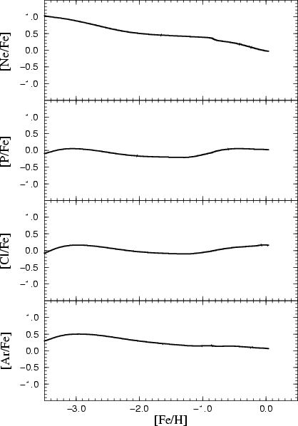
4.5 Neon, phosphorus, chlorine and argon

Although there are no observational data to compare with, we plot in Fig. 12 the calculated evolution of the noble gases neon and argon, as well as those of phosphorus and chlorine, just for completeness.

Neon abundance is dominated by ²⁰Ne, and the three argon isotopes are also of even Z. Therefore, both elements should behave as $\alpha$ -elements. The calculations confirm this theoretical expectation. The evolution of neon in the halo-thick disk shows a clear dependence on metallicity, reminding of the oxygen behavior. For argon the metallicity effect is less marked, and its evolution reminds that of intermediate $\alpha$ -elements like silicon or calcium. In the absence of stellar observations for these elements, it is gratifying that their solar abundances are well reproduced.

Both odd-Z elements, phosphorus and chlorine, present solar or slightly subsolar abundance ratios in the halo-thick disk. When the assembling of the thin disk begins, their abundances gradually climb towards the solar values due to the odd-even effect in massive stars (and in a much lesser extent, by contribution of Type Ia supernovae), until the iron from Type Ia supernovae flattens the evolution of phosphorus, although it is not the case for chlorine.

$\begin{figure} \resizebox*{\hsize}{!}{\includegraphics{MS10620f13.eps}}\end{figure}$	Figure 13: Evolution with metallicity of the iron peak elements scandium, titanium and vanadium as a function of [Fe/H]
Open with DEXTER

4.6 The iron peak elements scandium, titanium, vanadium, chromium, manganese, cobalt and nickel

All these elements are basically synthesized through explosive burning in Type II and/or Type Ia supernova explosions, and some of them can also be produced by neutron captures during hydrostatic He and C burning. Their stellar yields are therefore much more uncertain than those of the intermediate-mass elements studied above, due to our deficient understanding of the parameters that characterize supernova explosions (energy and mass cut in Type II supernovae, progenitors, burning propagation and rates of Type Ia supernovae), and of neutron fluxes in hydrostatic He and C combustion. Isotopes with A 56 are mainly produced in explosive O and Si burning, and in Nuclear Statistical Equilibrium (NSE), while isotopes with $A\geq 56$ are produced in the alpha-rich freeze-out of NSE, besides contributions from neutron captures.

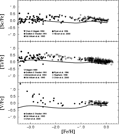
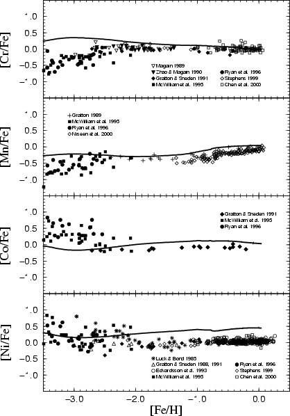
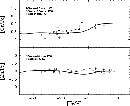
The calculated history of scandium, titanium and vanadium is displayed in Fig. 13, and that of chromium, manganese, cobalt and nickel appears in Fig. 14.

The evolution of the [Sc/Fe] ratio agrees reasonably well with the data for halo stars, characterized by a flat and nearly solar value, although between [Fe/H] = -2.5 and [Fe/H] = -1 we get a gentle decrease and our results fall below the observations. At the transition to the thin disk, the abundance grows slightly, as expected for an odd element, but iron from Type Ia supernovae, which make little scandium, overwhelms this increase and lowers the ratio [Sc/Fe], which is still below solar, during the disk evolution.

Titanium, dominated by ⁴⁸Ti, should behave as an $\alpha$ -element. In fact, the observations point to [Ti/Fe] $\sim$ 0.3-0.4 in the most metal-poor halo stars, and to a clear trend towards a declining ratio as metallicity increases. Loosely speaking, our calculations reproduce such characteristics, but the abundance is systematically lower than observed for the complete range of metallicity. At the solar birth all the titanium isotopes except ⁴⁶Ti are underabundant (see Fig. 5). TWW1995 and GP2000 found the same problems with titanium. The conclusion that current yields from massive stars alone fail to explain the titanium history is unavoidable.

The isotope ⁵¹V is predominant in the total abundance of vanadium. The few available data show a [V/Fe] flat and solar in population I and in metal-rich halo stars, and a tendency to increase as [Fe/H] decreases from -2 to -3. The calculations give a flat [V/Fe] in the halo-thick disk with a value of $\sim -$ 0.3, a moderate and rapid rise at the beginning of the thin disk formation, and a flat evolution slightly lower than solar during most of the thin disk phase; here, again, iron from Type Ia supernovae compensates the vanadium produced by massive stars with $Z \geq 0.1~Z _{\odot }$ .

The observations on the ratio [Cr/Fe] available until mid-nineties showed a constant and solar value down to [Fe/H] $\sim -$ 2.5, i.e. the same behavior as iron, indicating that both elements were produced in the same scenarios. However, recent observations show that the chromium abundance ratio to iron decreases as the metallicity goes down from [Fe/H] = -2.5 to [Fe/H] = -3.5, reaching at the latter metallicity values as low as [Cr/Fe] $\sim -$ 0.7. The chromium stellar yields of WW1995 are quite insensitive to Z. Our results, shown in Fig. 14, give an almost flat [Cr/Fe] in the complete range of metallicities, and thus fail to reproduce the data at low metallicity. The flatness of the abundance ratio is more marked in the disk because chromium and iron are produced in the same proportions by Type Ia supernovae, fitting precisely the solar abundances of the chromium isotopes.

In the case of manganese, with only one stable and odd-Z isotope ( ⁵⁵Mn), the calculated evolution fits well the data for [Fe/H] > -2.5, although in the thin disk there is an slight overabundance. The roughly linear increase in the disk reveals the odd-even effect for this element. At very low metallicities, as for chromium, the calculated abundances lie clearly above the data.

The observational situation for the ratio [Co/Fe] is rather puzzling. Cobalt is an odd element and therefore one expects its abundance to diminish with decreasing metallicity. Instead, the latest data point to a noticeable increase of its abundance at the lowest metallicities. We find a rough agreement down to [Fe/H] =-2.5, where [Co/Fe] mildly declines when going to lower metallicities, although the calculated history appears to lie higher than the observations. Below [Fe/H] =-2.5, the abundance ratio continues its gentle decline, just the opposite trend to that observed.

Nickel abundances in halo and disk stars have been obtained in a large number of surveys. Most of them show a constant and solar value for the ratio [Ni/Fe] at all metallicities, but the most recent observations seem to indicate an increasing ratio towards low [Fe/H], although the scatter is really large. The models give a continuous increase of an overabundant [Ni/Fe] for [Fe/H] > -3. We obtain higher values than observed due to the combination of a reduction by a factor of two in the WW1995 iron yields from massive stars, together with the large amount of ⁵⁸Ni in the yields of the W7 model of Type Ia supernovae, the latter being responsible for the positive slope in the thin disk.

4.7 Beyond the iron peak: Copper and zinc

These two elements are produced in significant amounts at different burning stages in massive stars. As for the iron peak elements, the total ejected amounts of these nuclei are strongly dependent on the characteristics of the supernova explosions. Nevertheless, ratios relative to iron could be less affected by astrophysical uncertainties. For instance, as shown by WW1995, in the explosion of a solar metallicity 35 $M _{\odot }$ model, variations by a factor of 2 in the explosion energy give changes in the [Ni/Fe] ratio of less than 10%. This argument in favor of the relative robustness of the calculated evolution of the element ratios relative to iron also applies to copper and zinc. The evolution of both elements is presented in Fig. 15.

Observations for these elements are scarce because they do not present enough suitable transitions. According to the available data, copper behaves like a typical odd nucleus, with a marked odd-even effect which gives a continuous growth of [Cu/Fe] with the iron contents. Our model nicely fits the data. At low metallicities we obtain a flat evolution, and in the thin disk the odd-even effect is clearly seen. As shown in Fig. 5, the solar abundances of the two copper isotopes are well adjusted.

The data for the zinc abundance show that this element evolves as iron, with a constant and solar [Zn/Fe] in the complete interval of observed metallicities. Here, again, the calculated evolution fits well the data. However, this result could be misleading since even if we obtain an elemental abundance in almost perfect agreement with the solar value, the distribution between the four isotopes of zinc (see Fig. 5) does not agree with the solar isotopic ratios. As mentioned above, we underproduce by a factor of $\sim$ 2 the most abundant isotope, ⁶⁴Zn, and overproduce ⁶⁸Zn by the same factor.

5 Summary and conclusions

We have analyzed the evolution of all the stable isotopes between hydrogen and zinc (lithium, beryllium and boron isotopes will be treated in a future paper) by means of a detailed chemical evolution code. In the framework of standard chemical evolution models only the works by TWW1995 and by GP2000 have studied such a large number of isotopes. In the first paper, the model employed was adequate just for the galactic disk evolution, apart from using the rather old yields of Renzini & Voli (1981) for low- and intermediate-mass stars. In the second case, even if the halo and the disk were correctly treated, only yields from massive stars were included

Our model assumes the formation of the Milky Way in two main episodes of exponentially decreasing infall. The first episode forms the halo and the thick disk from infall of primordial extragalactic material with an e-folding timescale of 1 Gyr. Then, the thin disk is assembled by infall of metal-rich extragalactic gas with a global metallicity of $0.1~Z _{\odot }$ in solar proportions, and with a relatively long timescale (7 Gyr at the solar ring). We have also calculated models that accrete material of primordial composition during the complete evolution. Although the results of the two kind of models are similar, we obtain a better agreement with the data for the stellar distribution of metallicities in the case of the model with enriched infall. We have employed an up to date IMF (the version of Kroupa et al. 1993), and a form for the SFR (the Dopita & Ryder's 1994 law), that relies on observations of the properties of star formation in spiral galaxies.

One important characteristic of our model is that it incorporates metallicity-dependent yields for isolated stars in the whole range of stellar masses. We use the WW1995 yields for massive stars and van der Hoek & Groenengen (1997) for low and intermediate-mass stars. Following TWW1995, in order to obtain a better concordance with observations, we have reduced the rather uncertain iron yield of WW1995 by a factor of two. We have not included metallicity effects in the yields of Type Ia supernovae, but GP2000 pointed out that the inclusion of the metallicity dependent yields of Iwamoto et al. (1999) hardly affects the final results. Finally, we have taken into account the nucleosynthetic contributions from novae that give important contributions to isotopes such as ¹³C, ¹⁵N, and ¹⁷O.

We have compared in detail the theoretical results with a large ensemble of observational data. First of all, in Sect. 3 we have shown that our results are able to reproduce the main characteristics of the solar vicinity, especially the G-dwarf distribution in the local disk, that we consider the most stringent restriction. We also obtain close agreement with the solar composition (both elemental and isotopic) at the time of 8.5 Gyr. It is worth stressing that:

Galactic chemical abundance evolution in the solar neighborhood up to the iron peak

1 Introduction