1 - Department of Physics, Ochanomizu University, 2-2-1 Otsuka, Bunkyo, Tokyo 112-8610, Japan
2 - Institute for Gender Studies, Ochanomizu University, 2-2-1 Otsuka, Bunkyo, Tokyo 112-8610, Japan
3 - Meteorological Research Institute, 1-1 Nagamine, Tsukuba 305-0052, Japan

Abstract
The Las Campanas Redshift Survey data are used to investigate structures ofthe galaxy number distribution. We construct two volume-limited samples with sizes of $113 \times 113$ and $126 \times 126$ h^-1 Mpc, and calculate the second- to ninth-order moments with the count-in-cell method. The galaxy distribution at $\ge$ 30 h^-1 Mpc is found to be statistically homogeneous. On the other hand, we find a multifractal scaling at <30 h^-1 Mpc. From the scaling exponent, we obtain the generalized dimension, which decreases from 2 toward 1 as the order is increased from 2 to 9. Galaxies are known to lie, around voids, in planar structures with filamentary dense regions. The present result indicates that these void-filament structures are predominant up to 30 h^-1 Mpc. Statistically, they appear to be the largest-scale significant structures in the Universe.

Key words: cosmology: observations - large-scale structure of Universe - methods: statistical

The galaxy number distribution at large scales ( $\gg$ 10 Mpc) is expected to be homogeneous. For example, the X-ray background emission, which originates in distant active galactic nuclei, is isotropic on the sky (e.g. Peebles 1993). Recently, several deep redshift surveys were carried out. The two-point correlation function and power spectrum based on these data indicate that the galaxy distribution actually becomes homogeneous at large scales (e.g. Wu et al. 1999; Martínez 1999). On the other hand, at small scales, the distribution is not homogeneous. Galaxies are distributed roughly on the walls of spherical voids, and show various spatial patterns such as groups, clusters, filaments, and sheets (e.g. Geller & Huchra 1989). At what scale are these structures predominant? Is there any other structure greater in scale? To answer these questions, we have to study the galaxy distribution in detail.

One promising approach to statistically describe the galaxy distribution is a "multifractal'' analysis, which characterizes scaling properties of moments at all the orders (Parisi & Frisch 1985; Jensen et al. 1985; Halsey et al. 1986; Sect. 3). The distribution is described more precisely than by the standard tools such as the two-point correlation function and power spectrum, which are based on the second-order moment alone. Kurokawa et al. (1999) studied galaxy data obtained from the CfA2 survey (Huchra et al. 1999), and found a multifractal scaling at $\le$ 20 Mpc (see also, e.g., Domínguez-Tenreiro et al. 1994; Martínez & Coles 1994). However, because of limitation of the volume size of the CfA2 survey, Kurokawa et al. (1999) were unable to determine the entire scaling range. Of great interest is an analysis of the scaling property at >20 Mpc.

We analyze galaxy data of the Las Campanas Redshift Survey (LCRS). This is the largest complete survey carried out so far and is expected to reach the scale of homogeneity (Shectman et al. 1996, Sect. 2). The volume size of the LCRS data is greater than those in the previous multifractal analyses. Since, however, the LCRS consists of two-dimensional slices, we newly define a multifractal analysis on a two-dimensional section of the three-dimensional distribution (Sect. 3). We demonstrate that the galaxy distribution exhibits a multifractal scaling at <30 Mpc and is homogeneous at $\ge$ 30 Mpc (Sect. 4). This result is used to discuss the galaxy distribution as a function of scale (Sect. 5). Finally we discuss potential problems of our approach and future prospects (Sect. 6).

Throughout this paper, we use the Hubble constant H₀ = 100 h kms^-1Mpc^-1 and the deceleration parameter q₀ = 0.5. With these parameters, the distance to a galaxy is estimated from its recession velocity in the Local Group frame. We ignore the peculiar velocities of the individual galaxies. They are typically 300 km s^-1(Davis & Peebles 1983), which corresponds to 3 h^-1 Mpc. This scale is less than the scales of our interest (>5 h^-1 Mpc), where we find a multifractal distribution.

2 Data and sample

The LCRS provides the largest galaxy sample which has been obtained so far (Shectman et al. 1996). This survey consists of six thin strips on the sky, each of which is $1.5^{\circ}$ in declination, $80^{\circ}$ in right ascension, and made of $1.5^{\circ}\times 3^{\circ}$ beams. Thus, the survey volumes are essentially two-dimensional slices. There are 26418 galaxies, which were selected from photometry in the R-band. Their average redshift is $z \simeq 0.1$ . The most distant galaxy lies at $z \simeq 0.4$ .

When we analyze the LCRS data, we encounter two problems. First, the LCRS has both upper and lower magnitude limits. They vary from beam to beam. To avoid the effect of this variation, our samples are constructed by applying the narrowest magnitude range to all the beams. Second, in the individual beams, redshifts of some galaxies were not measured. This was due to mechanical constraints of the spectrometer. Since the observed galaxies were selected randomly in the beam, we assigned the inverse of the number fraction of the observed galaxies as a statistical weight to each of the beams.

We extracted volume-limited samples, where the luminosities of the galaxies are above certain thresholds. The K-correction term was set to be K $(z) = 2.5 \log(1+z)$ , which provides a good approximation to the R-band data of LCRS galaxies (Lin et al. 1996a). We used the LCRS slices $\delta = -3^{\circ }$ and $-12^{\circ}$ . The other slices do not generate samples with sufficient numbers of galaxies. Our volume-limited samples contain the largest numbers of galaxies among those with thickness of 4 h^-1 Mpc. The sample from the slice $\delta = -3^{\circ }$ is complete in $16.1 \le m_R \le 17.1$ and $-21.4\le M_R \le -20.3$ , contains 173 galaxies, and is $113 \times 113~h^{-1}$ Mpc in size. Here m_R and M_R are the apparent and absolute magnitudes in the R-band. The sample from the slice $\delta = -12^{\circ }$ is complete in $15.1 \le m_R \le 17.6$ and $-21.7 \le M_R \le -20.6$ , contains 291 galaxies, and is $126 \times 126~h^{-1}$ Mpc in size. We underline that the volume sizes of these samples are greater than those used in previous multifractal analyses.

In the thickness direction, we applied a Gaussian window function in order to use the samples as two-dimensional cuts of the three-dimensional galaxy distribution (e.g. Landy et al. 1996). The full widths at half maximum of the window function are 0.6 and 0.5 h^-1 Mpc, respectively, in the samples for $\delta = -3^{\circ }$ and $-12^{\circ}$ . These widths are very small compared to the sample size, $\sim$ 100 h^-1 Mpc, and have been determined so as to reproduce most clearly the scaling properties of artificial fractal samples with the same number of discrete points as the LCRS data (Sect. 3).

We also studied the three-dimensional CfA2 sample (Huchra et al. 1999). Kurokawa et al. (1999) conducted a multifractal analysis of volume-limited samples with $M_{B(0)}\le -19.42$ and -20.00, which contain 358 and 194 galaxies and are $42 \times 42 \times 84$ and $54 \times 54 \times 108~h^{-1}$ Mpc in size. Their result for the CfA2 galaxies is compared with ours for the LCRS galaxies (Sect. 4). The LCRS and CfA2 observations were made in the R- and B(0)-bands. A typical LCRS galaxy is fainter in the B(0)-band by 1.8 mag that it is in the R-band (Lin et al. 1996a). That is, galaxies in our LCRS samples are less luminous than those in the CfA2 samples. Nevertheless, the luminosity difference does not adversely affect our analysis, because there are no gross differences in the distribution of galaxies at different luminosities (Huchra et al. 1990; Park et al. 1994).

3 Multifractal analysis on two-dimensional data

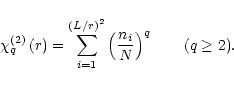
The formal definition of multifractal is not applicable to discrete sets. Hence, for analyses of the galaxy distribution, several different techniques have been proposed. They are reviewed and compared to each other in Ueda (1995). We employ the "count-in-cell'' method, which appears to be more straightforward than other methods. Since the LCRS samples are two-dimensional (Sect. 2), the present method is to infer a multifractal distribution in three-dimensional space from the distribution on a two-dimensional section.

Suppose that there are N galaxies on a square of size L. This square is divided into cells of size r. The qth moment $\chi_q^{(2)}$ at the scale r is defined as

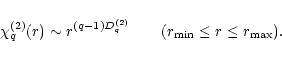
We plot $\log ( \chi_q^{(2)} )$ against $\log (r)$ . If the local slope is nearly constant over some range, there is said to be a scaling for that range:

$\begin{figure} \par\includegraphics[width=5.3cm,clip]{9487f1.eps} \end{figure}$

Figure 1: The fifth-order moments $\chi _5^{(2)}$ of Lévy fractal samples with D_f = 1.5 (open triangles) and D_f = 2.0 (filled triangles). The dotted lines represents the relations (2) expected for D_q⁽²⁾ = D_f -1

To justify our approach, we analyzed artificial monofractal samples, i.e., "Lévy flight'' sets with D_f = 1.5 and 2.0 (e.g. Mandelbrot 1982). The number of the points and the shape of the volume are the same as those of our LCRS sample for $\delta = -3^{\circ }$ . We applied the same Gaussian window as the LCRS sample, and calculated the moments $\chi _5^{(2)}$ . The average and standard deviation over 100 such samples are shown in Fig. 1. The moments $\chi _5^{(2)}$ follow the dotted lines, which represent the relation (2) with D_q⁽²⁾ = D_f -1. The same result is obtained if the point number, volume shape, and Gaussian window are the same as our LCRS sample for $\delta$ = $-12^{\circ}$ . Since the generalized dimensions ${D_q}^{(3)}\simeq 1.5-2.0$ were obtained in previous three-dimensional analyses of the galaxy distribution (e.g. Kurokawa et al. 1999), our method is expected to work well in the following analysis of the LCRS data.

However, in Fig. 1, the moments $\chi _5^{(2)}$ at $r/L \ll 0.1$ tend to lie above the dotted lines. They suffer from the finiteness of the point number. When the scale is very small and the number of cells is very large, every cell contains a single point at most. Even if the scale becomes smaller, the number of filled cells remains constant. The moments at these scales are simply proportional to the value N^1-q. This effect is less significant in the sample with D_f = 1.5. The reason is that a fractal structure has local clusters of points. The effective mean distance among the points is smaller in a fractal set with a smaller D_f value (Kurokawa et al. 1999).

4 Results

The moments $\chi_q^{(2)}$ of the two LCRS samples for $\delta$ = $-3^{\circ }$ and $-12^{\circ}$ are computed with q = 2-9 and r/L = 1/64-1/2. The results for $\delta = -3^{\circ }$ with q = 2, 5, and 9 are shown in Fig. 2 (filled squares). The scale r in units of h^-1 Mpc is indicated on the upper axes. The vertical bars on the moments represent the 1 $\sigma$ statistical errors evaluated with the "bootstrap resampling'' method (Efron 1982; Barrow et al. 1984).

$\begin{figure} \par\includegraphics[width=16.8cm,clip]{9487f2.eps} \end{figure}$

Figure 2: a) The second-order moments $\chi _2^{(2)}$ of the LCRS galaxy sample for $\delta = -3^{\circ }$ (filled squares). The solid line is the result of the least-squares fit at r = 5-20 h^-1 Mpc. The dotted line represents the relation expected for a homogeneous distribution. b) Same as a), but for the fifth-order moments $\chi _5^{(2)}$ . c) Same as a) but for the ninth-order moments $\chi _9^{(2)}$

Two scaling ranges are evident in Fig. 2. The transition from the one range to the other occurs within the scale interval of our analysis, which is roughly 0.5 in logarithms. The moments at $\ge$ 28 h^-1 Mpc lie on the dotted line, which represents the relation expected for a homogeneous distribution. The moments at <28 h^-1 Mpc exhibit another scaling. We apply the least-squares fit to the moments at the scales 7, 9, 14, and 19 h^-1 Mpc ( r/L = 1/16, 1/12, 1/8, and 1/6). The results are shown by solid lines. Below the scale 5 h^-1 Mpc, the moments do not follow the scaling relation. They suffer from the finiteness of the galaxy number (Sect. 3). The same results have been obtained for the other moments which are not shown in Fig. 2. We have also found a homogeneous distribution at r $\ge$ 32 h^-1 and another scaling relation at 5 < r < 32 h^-1 Mpc in the LCRS sample for $\delta = -12^{\circ }$ .

The generalized dimensions D_q⁽²⁾ for the moments at r< 28-32 h^-1 Mpc are derived from their scaling exponents, i.e., the slopes of the solid lines in Fig. 2. The values of D_q⁽³⁾ = D_q⁽²⁾ + 1 for $\delta = -3^{\circ }$ (filled squares) and $\delta = -12^{\circ }$ (filled circles) are plotted as a function of q in Fig. 3. We also show the generalized dimensions D_q⁽³⁾ of the CfA2 samples by open circles and squares (Kurokawa et al. 1999). The vertical bars on the data points represent the 1 $\sigma$ uncertainties associated with the least-squares fit, which incorporate the statistical errors of the individual moments. Within the 1 $\sigma$ uncertainties, the results for the four samples are consistent with each other. The D_q⁽³⁾ value decreases as q increases. Therefore, over the scale and order ranges considered here, the distribution of the LCRS galaxies satisfies the requirement for multifractal scaling.

$\begin{figure} \par\includegraphics[width=8cm,clip]{9487f3.eps} \end{figure}$

Figure 3: The generalized dimension D_q⁽³⁾ = D_q⁽²⁾ +1 for the LCRS galaxy samples with $\delta = -12^{\circ }$ (filled circles) and with $\delta = -3^{\circ }$ (filled squares). We also show D_q⁽³⁾ for the CfA2 galaxy samples with M_B(0) <-19.42 (open circles) and with M_B(0) < -20.00 (open squares)

We have presented only the galaxy moments $\chi_q^{(2)}$ with $q \le 9$ . The statistical errors of the higher-order moments are quite large. With an increase of q above 10, the generalized dimension D_q⁽³⁾ = D_q⁽²⁾+1 seems to converge to $D_{\infty}^{(3)} \simeq 1.5$ in both the samples for $\delta = -3^{\circ }$ and $-12^{\circ}$ . Their scaling ranges seem to be the same as those for $q \le 9$ . This result is again consistent with that for the CfA2 data, which exhibit $D_{\infty}^{(3)} \simeq 1.4$ (Kurokawa et al. 1999).

In summary, we have found a multifractal distribution at <30 h^-1 Mpc and a homogeneous distribution at $\ge$ 30 h^-1 Mpc. This result has been obtained from both the LCRS samples for $\delta = -3^{\circ }$ and $-12^{\circ}$ , agrees with the result for the CfA2 samples, and hence is expected to be general. Hereafter we separately discuss the multifractal and homogeneous distributions.

5 Discussion

5.1 Multifractal distribution at <30 Mpc

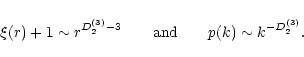
By using the two-point correlation function $\xi(r)$ , power spectrum p(k), or other multifractal techniques, it is possible to estimate the D₂⁽³⁾ value (e.g. Guzzo et al. 1991; Martínez & Coles 1994):

With increasing the order q, the D_q⁽³⁾ value decreases from 2.0 to 1.5 (Fig. 3). This decrease might be considered small, but it is significant. Since the higher-order moments give more weight to the dense regions, those D_q⁽³⁾ values are obtained if there are filament-like dense regions within sheet-like structures. The former has D_q⁽³⁾ $\simeq$ 1 while the latter has D_q⁽³⁾ $\simeq$ 2. Galaxies are known to lie roughly on the walls of spherical voids (e.g. Geller & Huchra 1989). From the topology of isodensity contours of CfA2 galaxies, Vogeley et al. (1994) found that their distribution forms "walls with holes'' or a "filamentary net''. Kurokawa et al. (1999) interpreted the multifractal distribution of the CfA2 data as originating in these void-filament structures. If this interpretation is correct, the present result indicates that the void-filament structures are important up to 30 h^-1 Mpc. The typical size of voids is actually known to be about 30 h^-1 Mpc (e.g. Peebles 1993).

The above structures can be generated via gravitational instability from primordial random fluctuations (e.g. Jenkins et al. 1998). With N-body simulations of cold dark matter models, Doroshkevich et al. (1999) showed richness of sheet-like structures with sizes of 20-30 h^-1 Mpc. To discriminate between different cosmological models, a comparison of the observed scaling with those of model predictions would be useful.

The observed multifractal scaling is unlikely to extend to the smaller scales ( $\ll$ $5\; h^{-1}$ Mpc). The value $D_2^{(3)} \simeq 2$ estimated for $r \simeq 5-30$ h^-1 Mpc is different from the value D₂⁽³⁾ $\simeq$ 1.2 obtained by Guzzo et al. (1991) for $r \le 3.5$ h^-1 Mpc (Table 1). These small scales correspond to a typical size of galaxy clusters. They are virialized systems, which originate in processes different to those for the void-filament structures. It is therefore natural to expect different scaling laws between scales above and below $\sim$ 3.5 h^-1 Mpc.

5.2 Homogeneous distribution at $\ge$ 30 Mpc

We have found D_q⁽³⁾ $\simeq$ 3 at $\ge$ 30 h^-1 Mpc. This result is consistent with those in Table 1. Thus, we conclude that the galaxy distribution at $\ge$ 30 h^-1 Mpc is homogeneous (e.g. Wu et al. 1999). The void-filament structures in Sect. 5.1 are the largest-scale spatial structure of the galaxy distribution. Here it should be noted that this conclusion is statistical. The largest void size in the CfA sample is $\simeq$ 50 h^-1 Mpc. The CfA sample also contains sheet-like structures such as the Great Wall and the Perseus-Pisces Supercluster, which are greater than 100 h^-1 Mpc in size (e.g. Geller & Huchra 1989). Such large-scale structures exist in our LCRS samples (Landy et al. 1996). However, the large-scale structures seem to be exceptional or of low amplitude and hence statistically unimportant in the present analyses. The LCRS data yield $\xi(r)$ $\simeq$ 0 at r $\simeq$ 30-250 h^-1 Mpc (Tucker et al. 1997; see also Martínez 1999). Kurokawa et al. (1999) studied CfA2 samples containing and not containing the Perseus-Pisces Supercluster, and found no significant diference in the multifractal statistics.

Sylos-Labini et al. (1998) claimed that the galaxy distribution has D₂⁽³⁾ $\simeq$ 2 up to 500 $\ h^{-1}$ Mpc. They ignored the K-correction. Scaramella et al. (1998) re-analyzed the same sample with the K-correction, and found a cross-over to homogeneity at several tens of h^-1 Mpc. When the K-correction is ignored, high-redshift galaxies are estimated to be less luminous. Their number density is underestimated in a volume-limited sample with a certain luminosity threshold. Even if the galaxy distribution is homogeneous, the neglect of the K-correction introduces a spurious structure in the redshift direction. To obtain the D₂⁽³⁾ value, both Sylos-Labini et al. (1998) and Scaramella et al. (1998) used the number of galaxies within the distance d: N(<d) $\sim$ d^{3-D₂⁽³⁾}. This quantity depends directly on the galaxy distribution in the redshift direction, and hence is sensitive to the K-correction (Joyce et al. 1999).

We, on the other hand, have divided a volume-limited sample into square cells, and investigated the number of galaxies in those cells. That is, we have studied the galaxy distribution not only in the redshift direction but also in the perpendicular direction. We expect that our analysis depends only weakly on the K-correction. To demonstrate this, we analyzed the LCRS data for $\delta$ = $-3^{\circ }$ with different K-correction terms. From spectral energy distributions of nearby galaxies, Fukugita et al. (1995) obtained relations between z and the K-correction as a function of morphological type. For spiral to elliptical galaxies, the K-correction term in the R-band is (1.3-5.0) $\times$ $\log(1+z)$ . We changed the K-correction term in this range, and calculated the moments $\chi _5^{(2)}$ . The results are shown in Fig. 4 (filled and open diamonds). They are consistent with reference lines, which are the same as in Fig. 2, at least in the multifractal and homogeneous regimes (r > 5 h^-1 Mpc).

**Table 1:** Estimates of the second-order generalized dimension D₂⁽³⁾
sample	D₂⁽³⁾	scale range^a	method^b	reference
		h^-1 Mpc
Perseus-Pisces	$1.25\pm0.10$	$(1) < r \le 3.5$	$\xi(r)+1$	1
CfA1	$1.23\pm0.04$	$0.1 < r \le 5$	$\xi(r)$	2
Perseus-Pisces	$2.21\pm0.06$	$3.5 \le r \le 25$ -30	$\xi(r)+1$	1
CfA1	$\simeq$ 2	$1 < r \le 30$	$(\xi(r)+1)n$	3
CfA1	$\simeq$ 2	$(1.5) \le r \le 20$ -30	multifractal^c	4
CfA2 ( $M_{B(0)}\le -19.42$ )	$1.95\pm0.08$	$(5) \le r \le (21)$	multifractal^d	5
CfA2 ( $M_{B(0)} \le -20.00$ )	$1.89\pm0.06$	$(7) \le r \le (27)$	multifractal^d	5
IRAS QDOT	2.25	$(1) \le r < 10$	multifractal^c	6
LCRS	$1.8\pm0.1$	5 < r < 30	p(k)	7
LCRS	$\simeq$ 2	$(4) < r \le 20$ -30	$\xi(r)+1$	8
LCRS ( $\delta$ = $-3^{\circ }$ )	$1.92 \pm 0.06$	(5) < r < 28	multifractal^d	9
LCRS ( $\delta$ = $-12^{\circ}$ )	$1.96 \pm 0.05$	(5) < r < 32	multifractal^d	9
Perseus-Pisces	$\simeq$ 3	25- $30 \le r < (70)$	$\xi(r)+1$	1
CfA1	$\simeq$ 3	20- $30 \le r \le (40)$	multifractal^c	4
IRAS QDOT	2.77	$10 < r \le (50)$	multifractal^c	6
LCRS ( $\delta$ = $-3^{\circ }$ )	$\simeq$ 3	$28 \le r \le (57)$	multifractal^d	9
LCRS ( $\delta$ = $-12^{\circ}$ )	$\simeq$ 3	$32 \le r \le (63)$	multifractal^d	9
Abell Clusters	$2.93 \pm 0.15$	$(70) \le r \le (300)$	N(<d)	10
ESO Slice Project	$3.08 \pm 0.18$	$(300) \le r < (500)$	N(<d)	10

Notes. (a) the value in parentheses is the analysis limit, which is determined by the volume or galaxy number of the sample; (b) $\xi(r)$ is the two-point correlation function, n is the mean number density, p(k) is the power spectrum, and N(<d) is the number of galaxies within the distance d; (c) the density reconstruction method; (d) the count-in-cell method.
References. (1) Guzzo et al. 1991; (2) Davis & Peebles 1983; (3) Lemson & Sanders 1991; (4) Domínguez-Tenreiro et al. 1994; (5) Kurokawa et al. 1999; (6) Martínez & Coles 1994; (7) Lin et al. 1996b; (8) Amendola & Palladino 1999; (9) this work; (10) Scaramella et al. 1998.

6 Concluding remarks

The scaling property of the galaxy number density has been explored through a multifractal analysis of the LCRS data. Since the LCRS is the largest complete survey carried out so far, our analysis is statistically more significant than the previous multifractal analyses. From the survey slices $\delta = -3^{\circ }$ and $-12^{\circ}$ , we have constructed two volume-limited samples. The former is complete in -21.4 $\le$ M_R $\le$ -20.3, contains 173 galaxies, and is 113 $\times$ 113 h^-1 Mpc in size. The latter is complete in -21.7 $\le$ M_R $\le$ -20.6, contains 291 galaxies, and is 126 $\times$ 126 h^-1 Mpc in size. The count-in-cell method on a two-dimensional section has been employed. At $\ge$ 30 h^-1 Mpc, the moments $\chi_q^{(2)}$ follow the scaling expected for a homogeneous distribution. On the other hand, from 5 to 30 h^-1 Mpc, we have found a multifractal scaling. The measured generalized dimensions D_q⁽³⁾ = D_q⁽²⁾+1 are consistent with those for the three-dimensional CfA2 galaxy samples. The results for D₂⁽³⁾ are also consistent with those obtained so far from various galaxy catalogues with $\xi(r)$ and p(k).

$\begin{figure} \par\includegraphics[width=4cm,clip]{9487f4.eps} \end{figure}$

Figure 3: The fifth-order moments $\chi _5^{(2)}$ of the LCRS galaxy samples for $\delta$ = $-3^{\circ }$ with K(z) = 1.3 $\log(1+z)$ (filled diamonds) and with K(z) = 5.0 $\log(1+z)$ (open diamonds). The reference lines are the same as in Fig. 4

These results are interpreted as follows. The galaxy distribution at $\ge$ 30 h^-1 Mpc is homogeneous. From 5 to 30 h^-1 Mpc, void-filament structures are predominant. Statistically, they are the largest-scale spatial structures of galaxy distribution. The multifractal scaling is unlikely to extend to small scales ( $\ll$ 5 h^-1 Mpc), where the structures are expected to be virialized.

Since the LCRS samples are two-dimensional, we have been unable to apply a three-dimensional analysis. The galaxy distribution in three-dimensional space has been inferred from the distribution in two-dimensional sections. However, the relation D_q⁽³⁾ = D_q⁽²⁾+1 is not applicable to all cases, although this relation is valid for Lévy flight sets that have nearly the same distribution as the galaxies. Moreover, there are structures much larger than 30 h^-1 Mpc in size. Our two-dimensional LCRS samples might have missed such structures by chance, or our multifractal method might be unable to detect them. For example, the two-dimensional power spectrum of the LCRS data exhibits a strong peak at $\simeq$ 100 h^-1 Mpc (Landy et al. 1996). We have ascertained that the present results for the two-dimensional LCRS data are consistent with previous analyses for the three-dimensional data (e.g. the CfA2 sample; Kurokawa et al. 1999), but it is important to confirm our results by analyzing a three-dimensional galaxy sample that is as deep as the present LCRS samples with various statistical methods. We hope that on-going redshift surveys such as the Sloan Digital Sky Survey will soon provide such galaxy data.

Scaling analysis of galaxy distribution in the Las Campanas Redshift Survey data

1 Introduction