4 Flux calibration

The goal of the flux calibration is to determine the spectral energy distribution above the atmosphere (the physical flux). The standard procedure to achieve the objective (Bessell 1999) consists of determining the instrumental response and correcting for the atmospheric absorption by comparing the spectra to templates of known spectral energy distribution observed with the same setup between the target stars.

Since the primary scope of the observation was not spectrophotometry, no particular care was taken in interleaving template stars and some observations were done through heavy atmospheric absorption. Therefore, the standard procedure cannot be straightforwardly applied.

The relation between the instrumental flux deduced in the previous section and the physical flux (the flux calibration relation) primarily reflects the effects of (1) the instrumental response (i.e. the combined effect of the whole optics and CCD spectral sensitivity), (2) the absorption by a clear atmosphere and (3) an additional extinction due to an atmospheric haze.

We started from the assumptions that (1) the instrumental response is stable or at least stable during each observing run, (2) the absorption by the clear atmosphere can be parameterized by the airmass and (3) the effect of the haze can be parameterized by a color excess defined as the difference between the measured B-V color and the Tycho-2 B-V color.

A fit of these three functions of the wavelength using spectra of stars with known spectral energy distribution (discussed below) resulted in a photometric precision of about 5% when we considered the instrumental response stable over all observation runs.

The shape of the three functions entering the calibration relation, and the analysis of the residuals, lead to the suspicion that the correction of the atmospheric refraction provided by the spectrograph was not fully effective. This was diagnosed by (1) a stronger than expected wavelength dependence of the apparent atmospheric and haze transmissions and (2) a residual random "curvature'' of the calibrated spectra that increases with airmass. Our interpretation is that the "clear atmosphere'' function corrects to a first order the effect of the refraction (the star is centered on the fiber aperture by the auto-guider on the blue end of the atmospheric spectrum). The uncertainty on the centering of the star (mis-guiding) results in a "color excess'' absorbed by the haze function, but depending on the value of the off-centering and of the seeing, a residual curvature remains.

It was unfortunately not possible to parameterize this effect since it depends on a random and unknown miss-centering and on the seeing which is not always recorded in the observing logs. An alternative would have been to use an additional color excess to constrain the curvature, but no such independent measurement is available for the stars of our archive.

Adding a quadratic airmass term, another function of color excess and allowing for variation of the instrumental response between the different observing runs led to a photometric quality of about 3% which was then improved to 2% after corrections based on internal comparisons. We did not find hints for other effect on the photometric quality, such as the effect of the stress on the optical fiber or positioning of the color correction filter that may change the instrumental response.

Finally, calibration consisted in: (1) primary calibration based on the comparison with low spectral resolution flux templates (2) secondary calibration based on internal comparison and (3) correction of the instrumental response using template spectra with a better spectral resolution than for the primary calibration.

4.1 Primary calibration

As already explained, the observations were not originally destined for photometry and no flux templates were explicitly observed. However, since the archive contains bright stars, many of them belong also to other libraries or datasets.

The largest intersection is with the collection of low resolution spectra presented in Burnashev (1985, CDS III/126). The spectral resolution is about R=100 ( FWHM = 5-6 nm), and the observations are from different sources which were homogenized to a common scale. The observations were done with photo-electric spectro-photometers mostly at the Crimean Observatory, and are not corrected for interstellar extinction.

Some stars in our archive are in common with other datasets with a better spectral resolution, but not in a number sufficient to fit the calibration relation. For this reason we chose to first calibrate the archive with this dataset. It was entered in the Hypercat Fits Archive (HFA) with the identification L1985BURN.

The first step was to assess the photometric quality of these templates. The B and V magnitudes were integrated on the spectra and compared with the measurements converted from the Tycho-2 catalogue. We found a rms difference on B-V of 0.05. The difference with the Tycho-2 color is used to assign a weight to each of these template observations.

The determination of the calibration relation is done after the instrumental spectra from our archive are convolved to the resolution of L1985BURN. The original reference does not precisely document this resolution which varies with the origin of the observations, and we had to determine it. A first guess was obtained by fitting Gaussians on strong Balmer lines and this was fine-tuned afterwards to minimize the residuals on the strong lines. It was necessary to adopt slightly different resolutions for the blue and red parts of the spectra.

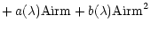
The model adopted for the primary calibration relation is:

$$\log(F_{\rm phys}(\lambda)) \log(F_{\rm inst}(\lambda)) + \log(F'_{\rm inst}(\lambda, {\rm run}))$$ =

$$+ \, a(\lambda) {\rm Airm} + b(\lambda) {\rm Airm}^2$$

$$+ \, c(\lambda) E_{B-V} + d(\lambda) E'_{B-V}.$$ (1)

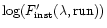$F_{\rm phys}$ is the physical flux reduced above the atmosphere. The two right-hand terms $\log(F_{\rm inst}(\lambda)$ and $\log(F'_{\rm inst}(\lambda,{\rm run}))$ represent the instrumental response. The first is stable over all the observing runs while the second is variable. We separated the two terms because the second could not be determined for all the observing runs: when the number of calibrated observations was less than 10 the second term was not computed and assumed to be 0. The run-dependent instrumental response was determined for 9 runs out of 21, and a secondary calibration (next sub-section) was also obtained.

The next two terms depend on the airmass (Airm). The first accounts for the clear atmosphere absorption and mean aperture effect due to the atmospheric extinction. The second partly corrects the "curvature'' of the spectrum due to the refraction (the length of the atmospheric spectra is proportional to $\tan z$, z being the zenithal distance).

The two last terms are parameterized by a B-V color excess, defined as the difference between B-V determined on our spectra and the Tycho-2 B-V.

It is not possible to measure directly the B magnitude on our spectra since the standard B band extends farther blue-ward than their limit. Hence it was necessary to "calibrate'' a different color, by fitting a color equation as is usually done to convert between photometric systems. This procedure has the disadvantage that it formally depends on the actual spectral energy distribution of the star and hence may introduce a bias linked to the atmospheric parameters of the stars. However, such an effect may be estimated from the residuals of the fit of the color equation, and for small color terms (i.e. if our internal B is close to the Johnson B) it can be neglected.

Since this conversion was necessary, we used this opportunity to define 2 B bands (b₁ and b₂, converted to Johnson scale as B₁ and B₂) giving two estimates of the color excess. The difference between these two estimates gives an approximate measure of the residual curvature of the spectra due to the atmospheric dispersion.

$$(B-V)_{\rm Tycho} - (B_1-V)_{\rm Elodie}$$ E(B-V) = (2)

E(B-V)' = B₂ - B₁. (3)

The B₁ and B₂ bands were respectively defined as the integral of the flux distribution between $\lambda\lambda = 450{-}470$ nm and $\lambda\lambda = 437{-}450$ nm.

The color equation was determined with the 2238 spectra of L1985BURN, using ordinary least squares and iterative rejection of outliers, as:

b₁ = 14.830 + 1.001 B₁ - 0.337 (B-V) (4)

b₂ = 15.195 + 1.003 B₂ - 0.081 (B-V). (5)

The rms residuals from these fits are about 0.025 mag. The magnitudes and colors are practically measured on the instrumental spectra (not physical flux), and hence the measured excess is biased due to the instrumental response and depends on the airmass. Though it does not change the fit to Eq. (1), in order to have independent functions we corrected the excess from the effect of instrumental response and atmospheric extinction using an a posteriori fit between corrected and un-corrected excess.

The flux calibration relation was fitted on 369 spectra of stars in common between our archive and L1985BURN. The different functions of the wavelength were finally smoothed by fitting polynomials in order to erase the residual effects of resolution mis-matching which results in spurious irregularities in these functions (in particular around H$_\gamma$ and G-band).

4.2 Secondary calibration

The primary calibration allowed us to determine the run-dependent response for only half the runs (but more than half the spectra since the number of stars is not equal in each run).

The inter-comparison of spectra of the same stars for which several observations were available allowed a secondary calibration. The runs where the run-dependent response was available were used as "template''.

This exercise allowed us to detect a significant change in the response of the instrument between the observations prior to 1995 and those done after. This change seems to be due to a modification of the differential refraction corrector at the end of year 1994. In addition, for two other runs the number of inter-comparisons was large enough to adopt a reliable run-dependent correction. The run-dependent corrections account for a rms photometric effect of about 0.025 mag. For 9 runs no such correction is available at present.

4.3 Correction of the instrumental response

Figure 3: The mean photometric residuals of the 9 libraries used for the correction of the instrumental response (before this corrections). The ordinate is the mean difference (Elodie - reference library) in units of relative physical flux (normalized to 1 at 555 nm). Each dataset is shown on a different line, each being arbitrary y-shifted by 0.05. From bottom to top they are: Jones (blue and red), Serote Roos et al. (OHP and CFH), Jacoby, Kiehling, Danks & Dennefeld, Gunn & Stryker and the Sun. For the purpose of the display these spectra have been slightly smoothed. The top line is the combination of all the individual comparisons which were used to compute the correction to the instrumental response

Up to this point the flux calibration can be assumed to properly correct the effect of atmospheric absorption and to correct at best the aperture effect due to the differential refraction. However, the instrumental response was evaluated using low-resolution spectra and furthermore had to be smoothed. At variance with the other functions which presumably vary smoothly with wavelength, the instrumental response may be more chaotic.

Therefore, the last step of the calibration process consists of using higher spectral resolution ( $R \approx 1000$) to correct the instrumental response. These reference spectra are taken from the following dataset, referenced by their HFA identification:

• L96111KP1 and L96111KP2. The ELODIE database contains 191 spectra of 144 stars from the Jones library (Leitherer et al. 1998) (R=2800). This library cover two narrow wavelength ranges, one in the blue part below $\lambda = 451$ nm the other between $\lambda \lambda= 478{-}547$ nm. This is the highest resolution reference for stellar spectra yet available for comparison. This library is not corrected for the aperture effect due to differential refraction and is not of photometric quality. After re-calibrating the "color'' of these spectra (defining special color-band as we did for our spectra for the primary calibration), the mean agreement with our spectra is satisfactory;

• L1996SERO. The ELODIE database has 8 spectra of 6 stars in common with Serote Ross et al. (1996). These spectra are from CFH (R=650) and OHP (R=4000) observations. They intersect the red half of our spectral range. The comparison with the L1996SERO spectra, after the spectral resolutions are matched by convolving our spectra with a Gaussian, show pixel-to-pixel variations of the order of 2% (rms) and low-frequency variations of typically 5%. These figures are consistent with the comparison performed by Serote Ross et al. (1996) with the Silva & Cornell (1992) library;

• L1984JACO. We have 2 spectra for 2 stars (HD 094028 & HD 028099) in common with the Jacoby library (R=1200) which cover the full wavelength range. The two spectra compared with L1984JACO reveal a significant gradient (the difference over the whole range of wavelength are respectively 29% and 14% for the first and second spectrum) and a pixel-to-pixel variation of 0.5% rms. The B-V color integrated from the L1984JACO spectra disagrees with the Tycho-2 value in amounts that explain the differences with our spectra;

• L1987KIEH. We have 13 spectra of 7 stars from the dataset of Kiehling (1987) (R=800);

• L1994DANK. We have 17 spectra from 14 stars in common with Danks & Dennefeld (1994) (R=1500). The red half of our wavelength range intersects with L1994DANK;

• L1983GUNN. The Gunn & Stryker (1983) library (R=500) counts 5 stars in common with our archive;

• L1984NSOA. We compared our 7 solar spectra with the Solar flux atlas (Kurucz et al. 1984) ( $R=500\,000$, also stored in HFA with $R=10\,000$).

We made all the individual comparisons between our spectra, convolved by a Gaussian to match the resolution, and these references. Because the broad-band variations are probably due either to random photometric errors in our archive (certainly not systematic), correction of the interstellar extinction (it was not always possible to de-correct the templates) or errors in the templates, we subtracted a low-degree polynomial (1 to 3 depending on the dataset) to these comparisons.

The individual comparisons (see Fig. 3) were then combined and produced a mean residual convolved to a resolution of 2 nm FWHM (each order of the original spectrum covers about 4 nm and no correction of the instrumental response at a lower scale is desired). This was used to correct the instrumental response.

Figure 4: Photometric precision deduced from the comparison of multiple observations of the same star. The ordinate are the rms of the 358 pair comparisons (ln(Flux2/Flux1)) (the spiky appearance is due to the logarithmic comparison). The higher curve is the total rms while the lower one is after third degree polynomials were subtracted from each individual comparison: this disentangles the effect of photon noise and uncertainty on the long range flux calibration (due to the differential refraction). To obtain the order of magnitude of the photometric error on single observation, the ordinates should be divided by $\sqrt {2}$

We also made an unsuccessful attempt to compare our archive with the Pickles (1998) library (L1998PICK): all the spectra were compared to the nearest (in the $\mbox{$T_{\rm eff}$ }- \mbox{$\log~g$ }- \mbox{[Fe/H]}$ space) template in L1998PICK. But the mapping of the parameters space in L1998PICK is not dense enough and the residuals are too affected by the distance in the parameter space to permit a useful analysis. We did not attempt to interpolate the spectra within the Pickles library.