A&A 369, 49-56 (2001)
DOI: 10.1051/0004-6361:20010102
Soft X-ray AGN luminosity function from ROSAT surveys
II. Table of the binned soft X-ray luminosity function
T. Miyaji 1,2,3 - G. Hasinger 3 - M. Schmidt 4
1 - Department of Physics, Carnegie Mellon University, Pittsburgh, PA 15213, USA
2 -
Max-Planck-Inst. für Extraterrestrische Physik, Postf. 1603,
85740 Garching, Germany
3 -
Astrophysikalisches Institut Potsdam, An der Sternwarte 16, 14482
Potsdam, Germany
4 -
California Institute of Technology, Pasadena, CA 91125, USA
Received 14 June 2000 / Accepted 8 January 2001
Abstract
This is the second paper of our investigation of the
0.5-2 keV soft X-ray luminosity function (SXLF) of active galactic
nuclei (AGN) using results from ROSAT surveys of various
depth. The large dynamic range of the combined sample, from shallow large-area
ROSAT All-Sky Survey (RASS)-based samples to the
satellite's deepest pointed observation on the Lockman Hole, enabled
us to trace the behavior of the SXLF. While the first paper (Miyaji et al. 2000, hereafter Paper I) emphasized the
global behavior of the SXLF, cosmological evolution
and contribution to the soft X-ray background, this paper presents
actual numerical values for practical use of our results.
To present the binned SXLF, we have used an improved
estimator, which is free from biases associated with
the conventional
 estimator.
Key words: galaxies: active - galaxies: evolution -
(galaxies:) quasars: general -
X-rays: galaxies - X-rays: general
1 Introduction
The AGN/QSO luminosity function and its evolution with
cosmic time are key observational quantities for understanding
the origin of and accretion history onto supermassive black holes,
which are now believed to occupy the centers of most galaxies.
Since X-ray emission is one of the prominent characters of
the AGN activity, X-ray surveys are efficient means of sampling
AGNs for luminosity function and evolution studies.
An X-ray selected sample of AGNs is particularly useful
because optical surveys often use point-like morphology as a
criterion for selecting AGNs (QSOs) among numerous other
objects, and thus are likely to miss moderate-luminosity
intermediate-high redshift AGNs embedded in their host galaxies.
Also, radio surveys sample only a minor population of AGNs.
The Röntgen satellite (ROSAT)
provided us with soft X-ray surveys with various
depths, ranging from the ROSAT All-Sky Survey (RASS, Voges et al. 1999)
to the ROSAT Deep Survey (RDS) on the Lockman Hole (Hasinger
et al. 1998). Various optical identification programs
of the survey fields have been conducted and the combination
of these now enabled us to construct the soft X-ray luminosity
function (SXLF) as a function of redshift.
In Paper I, we presented a number of
global representations of the 0.5-2 keV SXLF and investigated
the contribution to the soft X-ray background.
We showed that our data are not consistent with
the pure-luminosity evolution (PLE), contrary to
the suggestions of a number of previous analyses (e.g. Boyle et al.
1994; Jones et al. 1996). Instead,
we find an excess of intermediate-redshift low-luminosity
AGNs above the PLE case, some sign of which was also recognized
by Page et al. (1997). In view of this, we developed
two versions of luminosity-dependent density evolution
(LDDE1 and LDDE2) models, which represent the observed data
very well. An extrapolation of these two LDDE models below the faintest
limit of the survey (

![$[{\rm erg\,s^{-1}\,cm^{-2}}]$](/articles/aa/full/2001/13/aa1904/img5.gif) )
yields significantly different predictions
for fainter fluxes, bracketing the range of a possible AGN
contribution to the soft X-ray Background.
Chandra (e.g. Mushotzky et al. 2000;
Hornschemeier et al. 2000) and XMM-Newton (2001)
are probing much fainter sources and spectroscopic identifications
of these will eventually show which of these models is closer to the
actual behavior of the AGN SXLF. However, because at least some of the
faint X-ray sources are optically too faint for spectroscopic
identification even with the largest telescopes, extending the XLF into
such faint flux level may be difficult.
In this second paper, we present practical and convenient
expressions of the observed SXLF from the ROSAT
surveys. We present our results mainly for the investigators who
are interested in particular redshift regimes
and/or comparing their models with observations.
)
yields significantly different predictions
for fainter fluxes, bracketing the range of a possible AGN
contribution to the soft X-ray Background.
Chandra (e.g. Mushotzky et al. 2000;
Hornschemeier et al. 2000) and XMM-Newton (2001)
are probing much fainter sources and spectroscopic identifications
of these will eventually show which of these models is closer to the
actual behavior of the AGN SXLF. However, because at least some of the
faint X-ray sources are optically too faint for spectroscopic
identification even with the largest telescopes, extending the XLF into
such faint flux level may be difficult.
In this second paper, we present practical and convenient
expressions of the observed SXLF from the ROSAT
surveys. We present our results mainly for the investigators who
are interested in particular redshift regimes
and/or comparing their models with observations.

Abbreviations - RBS: The
ROSAT Bright Survey
(Fischer et al.
1998; Schwope et al.
2000),
SA-N: The Selected Area-North (Zickgraf et al.
1997;
Appenzeller et al.
1998), RIXOS: The
ROSAT International
X-ray Optical Survey (Mason et al.
1999), NEP: The North Ecliptic
Pole Survey (Bower et al.
1996);
UKD: The UK Deep Survey (McHardy et al.
1998),
RDS-Marano: The
ROSAT Deep Survey - Marano field
(Zamorani et al.
1999,
RDS-LH: The
ROSAT Deep
Survey - Lockman Hole (Hasinger et al.
1998;
Schmidt et al.
1998; Lehmann et al.
1999).

Excluding AGNs with
z<0.015.
For this purpose, we show convenient analytical
expressions in several redshift intervals separately.
These give more accurate representations of the data
in the redshift ranges of interest than those presented
in Paper I. We also tabulate the numerical values of
the binned SXLF using an improved estimator.
We use a Hubble constant

![$[{\rm km\,s^{-1}\,Mpc^{-3}}]$](/articles/aa/full/2001/13/aa1904/img13.gif) .
The h50 dependences are explicitly shown. We calculate
the results with common sets of cosmological parameters:
.
The h50 dependences are explicitly shown. We calculate
the results with common sets of cosmological parameters:
 ,
(0.3,0.0).
and
,
(0.3,0.0).
and
 .
The symbol "
.
The symbol " '' represents the base-10 logarithm.
2 The summary of the sample
We have used soft X-ray sources identified with
AGNs with redshift information from a combination of ROSAT
surveys in various depths/areas from a number of already
published and unpublished sources. Detailed description of
the definition of the sample, ROSAT
countrate-to-flux conversion, and survey area are
shown in Paper I. The summary of the samples, which is
a duplicate of Table 1. of Paper I with updated references, is
shown in Table 1. The details of the nature
and completeness of each sample were discussed in Paper I.
The limiting flux versus survey area relation were also
shown in Paper I.
As in Paper I, we present the SXLF in the observed
0.5-2 keV band, i.e., in the
0.5(1+z)-2(1+z)keV range in the object's rest frame. This is equivalent
to assuming an energy index of 1.
Thus no K-correction was applied for our expressions presented here.
The reasons for this choice are explained in detail in Paper I.
This choice is particularly important for this paper, which
is intended to be used as observational constraints for
population-synthesis-type models (e.g. Madau et al. 1994;
Comastri et al. 1995; Gilli et al. 1999, 2000;
Miyaji et al. 2000) with various spectral
assumptions. Because of that, it is more useful to provide
quantities in a model-independent form rather than
applying a particular version of model-dependent K-corrections.
By presenting the data in this manner, one can avoid the difficulty
of reverse K-correcting and re-applying new K-corrections when the
new results from Chandra and XMM provide
better knowledge of the X-ray spectra of the population.
3.1 Analytical expressions
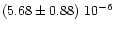
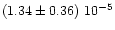
Table 2:
Best-fit parameters for each redshift bin
| z-range |
 |
N |
 |
 |
 |
 |
p |
KS-prob |
 |
|
0.015-0.2 |
0.1 |
269 |
 |
0.60
+0.68-0.32 |
0.59
+0.23-0.29 |
2.1
+0.4-0.3 |
4.22
+2.53-2.61 |
0.99, 0.68, 0.61 |
| 0.2-0.4 |
0.3 |
113 |
 |
0.89
+1.20-0.46 |
0.67
+0.30-0.38 |
2.5
+0.4-0.3 |
5.25
+3.48-3.51 |
0.93, 0.56, 0.72 |
| 0.4-0.8 |
0.6 |
99 |
 |
0.54
+0.85-0.29 |
0.33
+0.52-0.87 |
2.2
+0.3-0.2 |
5.95
+2.29-2.29 |
0.85, 0.85, 0.57 |
| 0.8-1.6 |
1.2 |
135 |
 |
1.48
+1.14-0.56 |
0.40
+0.41-0.53 |
2.4
+0.2-0.2 |
4.07
+1.33-1.34 |
0.99, 0.96, 0.83 |
| 1.6-2.3 |
2.2 |
44 |
 |
1.2(*) |
0.0(*) |
2.1
+0.2-0.1 |
0(*) |
0.27, 0.36, 0.19 |
| 2.3-4.6 |
3.0 |
25 |
 |
1.0(*) |
... |
1.9
+0.2-0.2 |
0(*) |
0.72, 0.99, 0.64 |
 |
|
0.015-0.2 |
0.1 |
269 |
 |
0.59
+0.71-0.32 |
0.59
+0.23-0.30 |
2.1
+0.4-0.3 |
4.13
+2.56-2.63 |
0.99, 0.60, 0.54 |
| 0.2-0.4 |
0.3 |
113 |
 |
0.93
+1.30-0.49 |
0.67
+0.31-0.39 |
2.4
+0.4-0.3 |
5.31
+3.49-3.51 |
0.99, 0.53, 0.79 |
| 0.4-0.8 |
0.6 |
99 |
 |
0.69
+1.07-0.36 |
0.37
+0.50-0.80 |
2.3
+0.3-0.2 |
5.90
+2.28-2.28 |
0.97, 0.81, 0.57 |
| 0.8-1.6 |
1.2 |
135 |
 |
2.14
+1.67-0.83 |
0.42
+0.40-0.52 |
2.4
+0.2-0.2 |
4.13
+1.34-1.34 |
0.98, 0.97, 0.72 |
| 1.6-2.3 |
2.2 |
44 |
 |
1.8(*) |
0.0(*) |
2.1
+0.2-0.1 |
0(*) |
0.19, 0.41, 0.15 |
| 2.3-4.6 |
3.0 |
25 |
 |
1.0(*) |
... |
1.9
+0.2-0.2 |
0(*) |
0.64, 0.96, 0.75 |
 |
|
0.015-0.2 |
0.1 |
269 |
 |
0.71
+0.86-0.39 |
0.62
+0.22-0.29 |
2.1
+0.4-0.3 |
3.79
+2.56-2.64 |
0.99, 0.54, 0.61 |
| 0.2-0.4 |
0.3 |
113 |
 |
1.09
+1.53-0.58 |
0.67
+0.30-0.39 |
2.4
+0.4-0.3 |
4.95
+3.49-3.51 |
0.97, 0.56, 0.82 |
| 0.4-0.8 |
0.6 |
99 |
 |
0.85
+1.41-0.46 |
0.36
+0.51-0.87 |
2.2
+0.3-0.2 |
5.69
+2.28-2.27 |
0.96, 0.81, 0.60 |
| 0.8-1.6 |
1.2 |
135 |
 |
2.69
+2.07-1.04 |
0.43
+0.39-0.51 |
2.4
+0.2-0.2 |
4.10
+1.33-1.34 |
0.98, 0.97, 0.74 |
| 1.6-2.3 |
2.2 |
44 |
 |
2.0(*) |
0.0(*) |
2.1
+0.1-0.1 |
0(*) |
0.14, 0.40, 0.16 |
| 2.3-4.6 |
3.0 |
25 |
 |
1.0(*) |
... |
1.9
+0.2-0.2 |
0(*) |
0.78, 0.98, 0.76 |
First, we find a smooth analytical
function for each redshift bin using a Maximum-likelihood
fitting.
The absolute goodness of the resulting expression can
then be tested by one- and two-dimensional Kolgomorov-Smirnov tests
(hereafter, 1D-KS and 2D-KS tests respectively; Press et al. 1992;
Fasano & Franceschini 1987).
See Paper I for detailed
description of these methods. These fittings and
tests can be applied to unbinned data sets thus are
free from artifacts and biases from binning.
For an analytical expression, we use the smoothed two-
power-law formula, as we did in Paper I. Here,
we fit the data in narrow redshift bins and thus evolution
in each redshift bin is assumed to be a pure density evolution
form:
![\begin{displaymath}\frac{{\rm d}\;\Phi\,(L_{\rm x},z) }{{\rm d\;Log}\;L_{\rm x}}...
...}
\right]^{-1} \cdot \left(\frac{1+z}{1+z_{\rm c}} \right)^p,
\end{displaymath}](/articles/aa/full/2001/13/aa1904/img44.gif) |
(1) |
where
is the central redshift of the bin. For the highest
redshift bin where the "break'' is not apparent, we have used
a single power-law form by neglecting the first term in the square
bracket in Eq. (1).
![\begin{figure}
\par\includegraphics[width=8.8cm,clip]{DS1904f1.eps}\end{figure}](/articles/aa/full/2001/13/aa1904/Timg45.gif) |
Figure 1:
The binned XLFs from a simulated sample using
three different estimators (symbols with error bars as labeled) are
compared with the underlying "true'' XLF represented by dashed lines.
The vertical positions of the three different estimators have
been shifted vertically for display |
| Open with DEXTER |
The luminosity range of the fit is from
Log
 to the maximum available luminosity
in the sample. As shown below and in Paper I, the SXLF
below the minimum luminosity has a significant excess
above the smooth extrapolation. This excess smoothly
connects with the SXLF of the non-AGN population (e.g. Hasinger
et al. 1999) and the X-ray emission may be significantly
contaminated by non-AGN activities.
The set of parameters which give the best fit for each
redshift bin are shown in Table 2 along with
the results of the 1D- and 2D- KS tests (see the notes of the table).
The parameter errors correspond to a likelihood change of 2.7
(90% confidence errors). In any case, Eq. (1) gives
a statistically satisfactory expression for all redshift bins.
to the maximum available luminosity
in the sample. As shown below and in Paper I, the SXLF
below the minimum luminosity has a significant excess
above the smooth extrapolation. This excess smoothly
connects with the SXLF of the non-AGN population (e.g. Hasinger
et al. 1999) and the X-ray emission may be significantly
contaminated by non-AGN activities.
The set of parameters which give the best fit for each
redshift bin are shown in Table 2 along with
the results of the 1D- and 2D- KS tests (see the notes of the table).
The parameter errors correspond to a likelihood change of 2.7
(90% confidence errors). In any case, Eq. (1) gives
a statistically satisfactory expression for all redshift bins.
The
estimator, which is a generalized
version of the original
 estimator
(Schmidt 1968) applied to a sample composed
of subsamples of different depths (see Paper I; Avni & Bahcall
1980), has been widely used for binned luminosity
functions (LF; we use the acronym LF when the discussion is not limited
to the luminosity function in the X-ray band) in the literature.
However, as discussed in Paper I (see also
Wisotzki 1998; Page & Carrera 1999),
using it for a binned LF estimator can cause
significant biases, especially if the bin covers the flux range
where the available solid angle of the survey changes rapidly
as a function of flux. Also, the choice of the location
in a
estimator
(Schmidt 1968) applied to a sample composed
of subsamples of different depths (see Paper I; Avni & Bahcall
1980), has been widely used for binned luminosity
functions (LF; we use the acronym LF when the discussion is not limited
to the luminosity function in the X-ray band) in the literature.
However, as discussed in Paper I (see also
Wisotzki 1998; Page & Carrera 1999),
using it for a binned LF estimator can cause
significant biases, especially if the bin covers the flux range
where the available solid angle of the survey changes rapidly
as a function of flux. Also, the choice of the location
in a
 bin with a non-negligible width
at which the data point is plotted significantly changes the impression
of the plot.
In Fig. 3 of Paper I, however, we plotted the
estimates, because of the lack of a
reasonable alternative at the time of writing that paper, with
caveats on biases associated with the method.
We note that the estimator can be
used in an unbinned manner by considering a set of
delta-functions weighted by
bin with a non-negligible width
at which the data point is plotted significantly changes the impression
of the plot.
In Fig. 3 of Paper I, however, we plotted the
estimates, because of the lack of a
reasonable alternative at the time of writing that paper, with
caveats on biases associated with the method.
We note that the estimator can be
used in an unbinned manner by considering a set of
delta-functions weighted by
 (or
(or
 )
at the positions of sample objects in the luminosity space
(Schmidt & Green 1983), and this method is
free from biases mentioned above. While this unbinned method is
a powerful tool to predict, e.g., the source counts, it
does not provide practical means of plotting.
In this paper, we have developed an improved estimator,
which is explained in the next subsection.
)
at the positions of sample objects in the luminosity space
(Schmidt & Green 1983), and this method is
free from biases mentioned above. While this unbinned method is
a powerful tool to predict, e.g., the source counts, it
does not provide practical means of plotting.
In this paper, we have developed an improved estimator,
which is explained in the next subsection.
3.3 An improved estimator of the binned SXLF
As an alternative to the
method,
we have developed the following estimator for the binned
LF, which is free from most biases unavoidable
in the
method. In Sect. 3.1, we have
found a smooth analytical function which describes the behavior of the
SXLF in a given redshift range. Having the best-fit smooth function,
the estimated numerical value for the SXLF in a given
bin in the
 -space is:
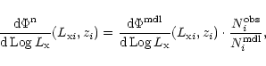 |
(2) |
where
 and zi are the luminosity and redshift
representative of the ith bin,
and zi are the luminosity and redshift
representative of the ith bin,
 is the best-fit analytical expression
evaluated at this point,
is the best-fit analytical expression
evaluated at this point,
 is the actual number
of AGNs observed in the ith bin, and
is the actual number
of AGNs observed in the ith bin, and
 is
the predicted number of AGNs in the bin from the best-fit
analytical expression. Hereafter, we refer to Eq. (2) as
the "
is
the predicted number of AGNs in the bin from the best-fit
analytical expression. Hereafter, we refer to Eq. (2) as
the "
 estimator''. Note that the estimator
proposed by Page & Carrera (1999) (hereafter PC) is a special
case of Eq. (2) where
estimator''. Note that the estimator
proposed by Page & Carrera (1999) (hereafter PC) is a special
case of Eq. (2) where
 (or
(or
 ).
).
Another advantage of this estimator over  is that
exact errors at a given significance can be evaluated using
Poisson statistics. One disadvantage of this estimator is that it
is model-dependent, at least in principle. Since our analytical
expressions are satisfactory representations in any case and the
estimator is not sensitive to the details of the underlying model, the
uncertainties due to the model dependence are practically negligible.
is that
exact errors at a given significance can be evaluated using
Poisson statistics. One disadvantage of this estimator is that it
is model-dependent, at least in principle. Since our analytical
expressions are satisfactory representations in any case and the
estimator is not sensitive to the details of the underlying model, the
uncertainties due to the model dependence are practically negligible.
In order to compare the goodness of the estimators,
we performed simulations. Using the actual best-fit model
for the 0.2<z<0.4 bin for
,
we generated a set of simulated AGNs. The number of
simulated AGNs are 10 times those of the actual sample in order
to reduce the Poisson errors.
Using the simulated AGNs and the actual flux-area relation of our
combined sample, we estimated binned SXLFs using three
different estimators:
,
(Eq. (2)) and that of PC.
The results are compared with the underlying SXLF, which was used to
generate the simulated AGNs, in Fig. 1. For the models
to evaluate
 ,
we used the re-fitted model using the
simulated sample rather than the original model. The
1
,
we used the re-fitted model using the
simulated sample rather than the original model. The
1 errors for the
(Eq. (2)) and the
PC estimators are Poisson errors calculated
using Eqs. (7) and (12) of Gehrels (1986). On the other hand,
the errors for the
estimator are from Eq. (3) of
Paper I and are inaccurate for bins with a small number of AGNs.
errors for the
(Eq. (2)) and the
PC estimators are Poisson errors calculated
using Eqs. (7) and (12) of Gehrels (1986). On the other hand,
the errors for the
estimator are from Eq. (3) of
Paper I and are inaccurate for bins with a small number of AGNs.
As shown in Fig. 1, the
estimator best represents the original model and no estimated
point deviates from the underlying model by more than 2.
The
estimator underestimates the XLF in
the lowest luminosity bin as found in PC.
We note that the PC estimator also systematically
underestimates the LF in this particular case of the underlying
model and the flux-area relation.
This is expected because their estimator implicitly builds in the assumption
as the underlying LF shape. This is much more weighted towards
higher luminosities than any part of the realistic AGN XLF.
Since the amount of this bias depends on the underlying model
and the flux-area relation, as well as the points in the bin where
the data are plotted, it is not surprising that the bias is not
apparent in Fig. 2 of PC. They have also compensated for this bias upon
comparing the estimated LF with
a model. Instead of correcting the estimated binned LF using a good
model (which our
estimator does), they calculated
the "model-expectated value of the estimator'' to compare
with the estimated value from the data.
Detailed investigation and comparison of these different
estimators in various cases are beyond the scope of this paper.
Judging from this simulation, the above discussion on biases, and that
the exact Poisson errors can be used for errors, we choose
to use the
estimator for our plots and tabulation.
![\begin{figure}
\par\includegraphics[width=17.2cm,clip]{DS1904f2.eps}\end{figure}](/articles/aa/full/2001/13/aa1904/Timg63.gif) |
Figure 2:
The binned SXLFs estimated by Eq. (2) are
plotted with Poisson errors corresponding to the significance
range of Gaussian 1
from Eqs. (7) and (12) by Gehrels
(1986). The data points and error estimates are more
accurate than Fig. 3 of Paper I. Different symbols
correspond to different redshift bins as indicated in the lower-left
part of panel a). The symbol attached to a downward arrow
indicates the 90% upper limit (corresponding to 2.3 objects) for
the bin with no AGN in the sample. The best-fit analytical
model for each redshift bin in the luminosity range used for the
fit is overplotted in dashed lines |
| Open with DEXTER |
Using the
estimator,
we revised the full SXLF plot (Fig. 3 of Paper I), as shown
in Fig. 2. Instead of connecting
the data points, we overplotted the analytical model for
each redshift bin.
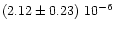
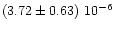
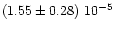
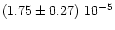
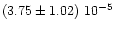
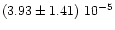
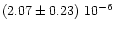
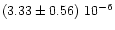
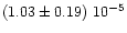
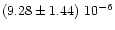
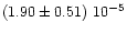
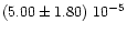
The resulting binned SXLF are listed in Tables 3, 4, and 5 for different sets of cosmological
parameters respectively.
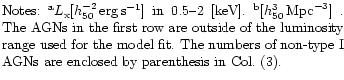
The columns of these tables are -- (1) the
redshift range of the bin; (2) the luminosity range of the bin;
(3) the number of AGNs in the sample for the bin and the number
of non-"type 1'' AGNs as defined in Appendix A of Paper I; (4) the
number of AGNs expected from the analytical model derived in
Sect. 3.1. (5) the binned SXLF estimated using Eq. (2)
using the model XLF evaluated at the central point of the bin, i.e.
 (see Table 2) and
 ,
where the subscripts min and max signify the borders of the bin
in Cols. (1) and (2). The upper and lower errors correspond to
Poisson errors estimated by Eqs. (7) and (12) of Gehrels (1986)
respectively using S=1 (corresponding to the confidence of the Gaussian
1.
When there is no object in the bin, the Poissonian 90%
confidence upper-limit is given (corresponding to 2.3 objects).
We recommend use of the values and errors under this column
when, e.g. overplotting observed SXLF values with model predictions
,
where the subscripts min and max signify the borders of the bin
in Cols. (1) and (2). The upper and lower errors correspond to
Poisson errors estimated by Eqs. (7) and (12) of Gehrels (1986)
respectively using S=1 (corresponding to the confidence of the Gaussian
1.
When there is no object in the bin, the Poissonian 90%
confidence upper-limit is given (corresponding to 2.3 objects).
We recommend use of the values and errors under this column
when, e.g. overplotting observed SXLF values with model predictions![[*]](/icons/foot_motif.gif) .
.
Figure 2 shows that the lowest-redshift, lowest-luminosity
bin has a significant excess over the two power-law analytical expression
(AGNs belonging to this bin have not been used for the two power-law fit),
thus the actual underlying SXLF has a much steeper slope than that used for
.
In order to evaluate the bias caused by this, we have made an
estimate of this particular bin using the
local slope of
 instead of
 from
the two power-law model. This gave a value about 10% lower, thus,
the difference is much smaller than the statistical errors for this
bin.
from
the two power-law model. This gave a value about 10% lower, thus,
the difference is much smaller than the statistical errors for this
bin.
We have shown the tables of observed SXLF values for a number of standard
set of cosmological parameters. These values are intended for
direct comparison with models and plotting with realistic
error bars. However, we list a number of caveats and sources of
uncertainties, and related issues.
- Countrate-to-flux conversion: For the PSPC-based observations,
where we can limit pulse-height channels, the uncertainty in the
countrate-flux (in 0.5-2 [keV]) conversion is small (
 3% for
photon spectral index of
3% for
photon spectral index of
 .
At the faintest
end (
.
At the faintest
end (
 ), where only the HRI data are available, the
conversion rate varies by
), where only the HRI data are available, the
conversion rate varies by  for the same spectral index range.
- Optical classification of AGNs: Since different catalogs used
in this analysis have different criteria for type I and type II
AGNs, we did not show separate expressions for these two populations.
See Appendix A. of Paper I for the approximate difference in behavior
of the tentative "type I'' sample.
- Incompleteness: Most of the surveys used in the analysis
are highly complete or we have selected an appropriate
complete subset. In case there is incompleteness, we have
corrected for it by assuming
that the redshift distribution/content of the remaining sources
are the same as the identified ones in the same flux range.
This assumption is not likely to be the case, considering that
they have not been identified not because of a random cause but
because of optical faintness and difficulty in obtaining decent
optical spectra. The only place that this could affect significantly
is the faintest end of RDS-LH (
 ), where
the identification completeness is 80%.
(At
), where
the identification completeness is 80%.
(At
 ,
the identification completeness
is
,
the identification completeness
is
 95% in any flux range). This could affect the behavior of,
e.g. the apparent break at the low luminosity end in
95% in any flux range). This could affect the behavior of,
e.g. the apparent break at the low luminosity end in
 .
.
- X-ray spectra/absorption: A serious model composer
should be aware that the luminosity given here is for
0.5-2 [keV] in the observer frame. Thus, one should compare the
model, with their own spectral assumptions (spectral index,
absorption, fraction of absorbed AGNs which may depend on
luminosity/redshift), should compute the apparent luminosity
in the
0.5(1+z)-2(1+z) [keV] range and compare it with the values
listed in this paper. The latest population synthesis
model based on absorbed and unabsorbed AGNs by Gilli et al.
(2000) has applied this approach using
the tables shown in this paper.
However, as discussed in Paper I, the no K-correction case corresponds
to a K-correction assuming a power-law photon index of
 ,
which is the most representative spectrum for the soft X-ray sources
in the sample. Thus for many purposes, considering our tabulated
values as K-corrected SXLF would be accurate enough.
,
which is the most representative spectrum for the soft X-ray sources
in the sample. Thus for many purposes, considering our tabulated
values as K-corrected SXLF would be accurate enough.
- Large-Scale Structure: The lowest redshift bin
covers 0.015 <z< 0.2 and there is some concern about the
effect of the large-scale structure of the universe, which could be
confused with the effect of evolution. Zucca et al. (1997) found
an underdensity of galaxies in the local universe out to
 .
However, it might be because of the structure within their
survey field of 27 [deg2] rather than that of the entire
space out to this redshift. The solid angle surveyed
by RBS is 50% of the sky and the fields of SA-N are scattered
in various directions. In any event, our lowest redshift bin samples
a sufficiently large volume of space to z= 0.2 with a uniform redshift
coverage, thus it is unlikely that the calculated SXLF is
significantly biased by the large-scale structure of the universe.
.
However, it might be because of the structure within their
survey field of 27 [deg2] rather than that of the entire
space out to this redshift. The solid angle surveyed
by RBS is 50% of the sky and the fields of SA-N are scattered
in various directions. In any event, our lowest redshift bin samples
a sufficiently large volume of space to z= 0.2 with a uniform redshift
coverage, thus it is unlikely that the calculated SXLF is
significantly biased by the large-scale structure of the universe.
Acknowledgements
This work is based on a combination of extensive ROSAT surveys
from a number of groups. Our work is indebted to the effort of the
ROSAT team and the optical followup teams in producing data
and the catalogs used in the analysis.
In particular, we thank K. Mason, A. Schwope,
G. Zamorani, I. Appenzeller, and I. McHardy for providing us with and
allowing us to use their data prior to
publication of the catalogs. TM was supported by a fellowship from the
Max-Planck-Society during his appointment at MPE. GH acknowledges
DLR grant FKZ 50 OR 9403 5. We thank the referee, T. Shanks, for
useful comments.
-
Appenzeller, I., Thiering, I., Zickgraf, F.-J., et al. 1998, ApJS, 117, 319
In the text
NASA ADS
-
Avni, Y., & Bahcall, J. N. 1980, ApJ, 235, 694
In the text
NASA ADS
-
Bower, R. G., Hasinger, G., Castander, F. J., et al. 1996, MNRAS, 281, 59
In the text
NASA ADS
-
Boyle, B. J., Shanks, T., Georgantopoulos, I., Stewart, G. C.,
& Griffiths, R. E. 1994, MNRAS, 271, 639
In the text
NASA ADS
-
Comastri, A., Setti, G., Zamorani, G., & Hasinger, G. 1995, A&A, 296, 1
In the text
NASA ADS
-
Fasano, G., & Franceschini, A. 1987, MNRAS, 225, 155
In the text
NASA ADS
-
Fischer, J.-U., Hasinger, G., Schwope, A. D., et al. 1998,
Astron. Nachr., 319, 347
In the text
NASA ADS
-
Gehrels, N. 1986, ApJ, 303, 336
In the text
NASA ADS
-
Gilli, R., Risalti, G. & Salvati, M. 1999, A&A, 347, 424
In the text
NASA ADS
-
Gilli, R., Salvati, M., & Hasinger, G. 2001, A&A, in press
[astro-ph/0011341]
In the text
-
Hasinger, G. 1996, A&AS, 120, C607
NASA ADS
-
Hasinger, G. 1998, AN, 319, 37
NASA ADS
-
Hasinger, G., Burg, R., Giacconi, R., et al. 1993, A&A, 275, 1
NASA ADS
-
Hasinger, G., Burg, R., Giacconi, R., et al. 1998, A&A, 329, 482
In the text
NASA ADS
-
Hasinger, G., Lehmann, I., Giacconi, R., et al. 1999,
in Highlights in X-ray Astronomy in Honor of
Joachim Trümper's 65th Birthday, MPE Report (Garching: MPE)
In the text
-
Hasinger, G., Altieri, B., Arnaud, M., et al. 2001,
A&A, 365, L45
In the text
NASA ADS
-
Hornschemeier, A. E., Brandt, W. N., Garmire, G. P., et al., ApJ, in press
[astro/ph-0042460]
In the text
-
Jones, L. R., McHardy, I. M., Merrifield, M. R., et al. 1996,
MNRAS, 285, 547
In the text
-
Lehmann, I., Hasinger, G., Schmidt, M., et al. 2000, A&A, 352, 35
In the text
-
Madau, P., Ghisellini, G., & Fabian, A. C. 1994, MNRAS, 270, L17
In the text
NASA ADS
-
Marshall, H. L., Avni, Y., Tananbaum, H., & Zamorani, G. 1983, ApJ, 269, 35
NASA ADS
-
Mason, K., Carrera, F. J., Hasinger, G., et al. 2000, MNRAS, 311, 456
In the text
NASA ADS
-
McHardy, I., Jones, L. R., Merrifield, M. R., et al. 1998, MNRAS, 295, 641
In the text
NASA ADS
-
Miyaji, T., Ishisaki, Y., Ogasaka, Y., Ueda, Y., et al. 1998, A&A, 334, L13
NASA ADS
-
Miyaji, T., Hasinger, G., & Schmidt, M. 1999, in Highlights in X-ray Astronomy
in Honor of Joachim Trümper's 65th Birthday, MPE Report (Garching: MPE),
in press [astro-ph/9809398], M99a
-
Miyaji, T., Hasinger, G., & Schmidt, M. 2000, A&A, 353, 25, Paper I
NASA ADS
-
Miyaji, T., Hasinger, G., & Schmidt, M. 2000, Adv. Sp. Res., 25, 827
In the text
NASA ADS
-
Mushotzky, R. F., Cowie, L. L., Barger, A. J., & Arnaud, K. A.
2000, Nature, 404, 459
In the text
NASA ADS
-
Page, M. J., Mason, K. O., McHardy, I. M., Jones, L. R., & Carrera, F. J.
1997, MNRAS, 291, 324
In the text
NASA ADS
-
Page, M. J., & Carrera, F. J. 1999, MNRAS, 311, 433
In the text
NASA ADS
-
Press, W. H., Teukolsky, S. A., Vetterling, W. T., & Flannery, B. P. 1992
Numerical Recipes in Fortran (Cambridge: Cambridge Univ. Press),
640
In the text
-
Schmidt, M. 1968, ApJ, 151, 393
In the text
NASA ADS
-
Schmidt, M, & Green, R. F. 1983, ApJ, 269, 352
the Universe, MPE Report 263 (Garching: MPE), 395
In the text
-
Schmidt, M., Hasinger, G., Gunn, J., et al. 1998, A&A, 329, 495
In the text
NASA ADS
-
Schwope, A. D., Hasinger, G., Lehmann, I., et al. 2000, Astr. Nachr., 321, 1
In the text
NASA ADS
-
Voges, W. 1994, in Basic Space Science, ed. H. J. Haubold, & L. I. Onuora,
202
-
Voges, W., Aschenbach, B., Boller, Th., et al. 1999, A&A, 349, 389
In the text
NASA ADS
-
Wisotzki, L. 1998, Astr. Nachr., 319, 257
In the text
-
Zamorani, G., Mignoli, M, Hasinger, G., et al. 1999, A&AS,
346, 732
In the text
-
Zickgraf, F.-J., Thiering, I., Krautter, J., et al. 1997, A&AS, 123, 103
In the text
NASA ADS
-
Zucca, E., Zamorani, G., Vettolani, G., et al. 1997, A&A, 326, 477
In the text
NASA ADS
Copyright ESO 2001
![\begin{figure}
\par\includegraphics[width=8.8cm,clip]{DS1904f1.eps}\end{figure}](/articles/aa/full/2001/13/aa1904/img45.gif)
![\begin{figure}
\par\includegraphics[width=17.2cm,clip]{DS1904f2.eps}\end{figure}](/articles/aa/full/2001/13/aa1904/img63.gif)