A&A 368, 749-759 (2001)
DOI: 10.1051/0004-6361:20010080
A. Finoguenov - T. H. Reiprich - H. Böhringer
Max-Planck-Institut für extraterrestrische Physik, Giessenbachstraße, 85748 Garching, Germany
Received 9 October 2000 / Accepted 20 December 2000
Abstract
We present results on the total mass and temperature determination using two
samples of clusters of galaxies. One sample is constructed with emphasis on
the completeness of the sample, while the advantage of the other is the use
of the temperature profiles, derived with ASCA. We obtain remarkably similar
fits to the M-T relation for both samples, with the normalization and the
slope significantly different from both prediction of self-similar collapse
and hydrodynamical simulations. We discuss the origin of these discrepancies
and also combine the X-ray mass with velocity dispersion measurements to
provide a comparison with high-resolution dark matter simulations. Finally,
we discuss the importance of a cluster formation epoch in the observed M-Trelation.
Key words: galaxies: clusters: general - cosmology: observations; dark matter; large-scale structure of Universe
There is increasing interest in using galaxy clusters characterized by X-ray observations as probes for cosmic structure and its evolution. In one of the applications, Press-Schechter models (Press & Schechter 1974) are used to constrain the shape and amplitude of the primordial density fluctuation spectrum at present day scales of 5 - 10 h-1 Mpc (e.g. Henry & Arnaud 1991; Oukbir & Blanchard 1992; Henry et al. 1992; Eke et al. 1996, 1998; Borgani et al. 1999). Another important measurement is that of the spatial correlations of X-ray clusters or, alternatively, the measurement of the power spectrum of the density fluctuations in the cluster density distribution (e.g. Nichol et al. 1992; Romer et al. 1994; Retzlaff et al. 1998; Miller & Batuski 2000; Schuecker et al. 2000; Collins et al. 2000). In both cases, the masses of the clusters have to be known for a large test sample in order to apply it to the structure analysis. The mass determination is still only feasible for a limited number of well-observed galaxy clusters, however. Therefore, in the above approaches the empirically-found correlation of the mass with the more easily observable parameters, X-ray luminosity or intracluster gas temperature, are used to make the connection between theoretical modeling and observations. The mass-temperature relation plays a crucial role in this analysis, since it was found to be particularly tight. Since the time of the first X-ray temperature measurements it was observed that the X-ray temperature is closely connected to the velocity dispersion of galaxies in clusters, indicating that both cluster components trace the cluster potential in a similar way (e.g. Mushotzky et al. 1978; Mushotzky 1984).
The validity of this approach was investigated in numerical calculations
based on N-body dynamic and hydrodynamic simulations making predictions on
the mass-temperature relation and its dispersion, as measured in X-ray
studies (Evrard et al. 1996; Evrard 1997). A close correlation
with a dependence of
![]() was predicted. It was found in this
work and also by e.g. Schindler (1996) that the X-ray mass determination
should be reliable (with an uncertainty in the range 14-29%). Evrard
et al. (1996 and Evrard 1997) argue, however, that the predicted
mass-temperature relation has such a small dispersion that a mass estimate
based on the temperature measurement only is more accurate than that
determined on the basis of the additional knowledge of the gas density
profile as obtained from
was predicted. It was found in this
work and also by e.g. Schindler (1996) that the X-ray mass determination
should be reliable (with an uncertainty in the range 14-29%). Evrard
et al. (1996 and Evrard 1997) argue, however, that the predicted
mass-temperature relation has such a small dispersion that a mass estimate
based on the temperature measurement only is more accurate than that
determined on the basis of the additional knowledge of the gas density
profile as obtained from ![]() -model surface brightness profile fits.
These predictions from simulations have been tested recently by means of
observational results by several authors (e.g. Böhringer 1995; Hjorth et al.
1998; Horner et al. 1999; Nevalainen et al. 2000). Disagreements have been
found concerning the predicted slope (see e.g. Horner et al. 1999; Nevalainen
et al. 2000) and the normalization of the mass-temperature relation.
-model surface brightness profile fits.
These predictions from simulations have been tested recently by means of
observational results by several authors (e.g. Böhringer 1995; Hjorth et al.
1998; Horner et al. 1999; Nevalainen et al. 2000). Disagreements have been
found concerning the predicted slope (see e.g. Horner et al. 1999; Nevalainen
et al. 2000) and the normalization of the mass-temperature relation.
At the time of writing, this discrepancy has not been solved, and various aspects of the data analysis and simulations have been discussed: the correct measurement of temperature gradients in the intracluster gas (e.g. Markevitch et al. 1998; Irwin et al. 1999; White 2000), influence of cooling flows (Allen 1998), non-thermal pressure support (e.g. Schindler 1996; Fukazawa et al. 2000), influence of the heating of the intracluster medium by supernovae (e.g. Balogh et al. 1999; Loewenstein 2000; Finoguenov et al. 2000, hereafter FAD), density and velocity bias in the galactic component of the cluster (Colín et al. 1999) and effects of numerical resolution in the simulations (Nevalainen et al. 2000).
In this paper we reinvestigate the observational mass-temperature relation using an extended sample of clusters with measured temperature profiles covering a wide range of systems with luminosity-averaged temperatures from below 1 up to 10 keV. In particular, we include 22 low temperature systems, thus improving on sampling the low-mass part of the M-T relation, compared to previous studies (e.g. Horner et al. 1999; Nevalainen et al. 2000). To study in detail the parameters that influence the normalization and the slope of the M-T relation, we rederive the M-T relation assuming an isothermal temperature distribution and also compare with the M-T relation for HIFLUGCS, a statistically complete sample of clusters, described in more detail below, where the isothermality assumption was the only choice. This sample is included in our study primarily to demonstrate that the result of the M-T relation is not affected by any selection bias. In addition, we discuss implications from the results of the M-T relation study on the epoch (redshift) of cluster formation.
The paper is organized as follows. In Sect. 2 we describe the
sample compilation, in 3 we compare the results obtained for
the two different samples, in 4 we combine the X-ray mass with
velocity dispersion measurements to provide a comparison with
high-resolution dark matter simulations and in 5 we discuss a
correction for the redshift of cluster formation. Unless noted otherwise, we
assume
![]() ,
,
![]() and 0,
and 0,
![]() g cm-3 throughout the paper.
g cm-3 throughout the paper.
In this paper we compare the M-T relation of two cluster samples. The
first is a statistically complete sample of the X-ray brightest clusters,
the HIghest X-ray FLUx Galaxy Cluster Sample (HIFLUGCS), for which the
selection criteria and thus possible bias effects are well defined. For this
sample, masses have been determined on the assumption of isothermality of
the X-ray emitting plasma. The second sample comprises those clusters for
which we have temperature profiles from ASCA observations and for which a
refined mass determination is possible. For the analysis of both samples, we
use the same definition of the ``total mass'' as the mass enclosed by the
radius, r500, inside which the mean cluster mass density is 500 times
higher than the critical density of the Universe. Accounting for the
observed redshift means that the critical density, used to calculate the
overdensity, is scaled for every cluster according to its redshift. Later,
in fitting the M-T relation, we correct the temperature of the cluster by
dividing by (1+z). These corrections mean that clusters form at different
epochs at similar overdensity, so
![]() .
Therefore, for a fixed mass
.
Therefore, for a fixed mass
![]() ,
and
,
and
![]() .
This is strictly correct only for
.
This is strictly correct only for
![]() .
However, correction for the observed redshift assuming lower values
of
.
However, correction for the observed redshift assuming lower values
of
![]() has even smaller effect on the derived parameters of the
M-T relation, so our correction, assuming
has even smaller effect on the derived parameters of the
M-T relation, so our correction, assuming
![]() ,
can be
considered as an extreme case. As we will show below, even in this case,
there is no difference in the results obtained for both cluster samples
considered here and thus no difference in the derived parameters of the
M-T relation is expected for any value of
,
can be
considered as an extreme case. As we will show below, even in this case,
there is no difference in the results obtained for both cluster samples
considered here and thus no difference in the derived parameters of the
M-T relation is expected for any value of
![]() .
.
Candidates for HIFLUGCS have been selected from recent cluster catalogs based
on the ROSAT All-Sky Survey. They have been reanalyzed homogeneously to
construct a complete X-ray flux-limited sample of the brightest clusters in
the sky, comprising 63 clusters. Details of the sample construction are
described in Reiprich et al. (2001). The cluster masses have been calculated
by assuming hydrostatic equilibrium and isothermality of the intracluster
gas and determining the gas density profile with the ![]() model
(Cavaliere & Fusco-Femiano 1976; Gorenstein et al. 1978; Jones & Forman 1984). Overall cluster temperatures have been compiled from the literature,
giving preference to temperatures measured with the ASCA satellite. The
cluster masses, M500 and the mass errors, determined by adding the
temperature error and the errors of the fit parameter values (
model
(Cavaliere & Fusco-Femiano 1976; Gorenstein et al. 1978; Jones & Forman 1984). Overall cluster temperatures have been compiled from the literature,
giving preference to temperatures measured with the ASCA satellite. The
cluster masses, M500 and the mass errors, determined by adding the
temperature error and the errors of the fit parameter values (![]() and
core radius), are tabulated in Reiprich et al. (2001). Since HIFLUGCS is purely
flux-limited, we avoid any bias that could be introduced in a subjectively
compiled sample, e.g. based on the most preferred targets selected for deep
observations. To maintain the completeness of the sample, out of 63 systems
in HIFLUGCS, for two we have to use estimated temperatures based on the L-Trelation by Markevitch (1998). We have checked, however, that excluding
these two systems from the fit does not change the derived parameters of the
M-T relation.
and
core radius), are tabulated in Reiprich et al. (2001). Since HIFLUGCS is purely
flux-limited, we avoid any bias that could be introduced in a subjectively
compiled sample, e.g. based on the most preferred targets selected for deep
observations. To maintain the completeness of the sample, out of 63 systems
in HIFLUGCS, for two we have to use estimated temperatures based on the L-Trelation by Markevitch (1998). We have checked, however, that excluding
these two systems from the fit does not change the derived parameters of the
M-T relation.
In addition, we will use also a larger sample (enlarged HIFLUGCS, 88 clusters), which is not strictly flux-limited, but contains only clusters with measured temperatures.
A linear regression is performed in log(T)-log(M) space. The method
allows for errors in both variables and intrinsic scatter (Akritas &
Bershady 1996). We use the bisector method to determine the best-fit
parameters (Isobe et al. 1990). Errors are transformed into log space by
![]() where x+ and x- denote the
upper and lower boundary of the quantity's error range, respectively. The
values of the fit parameters
are given in Table 1.
where x+ and x- denote the
upper and lower boundary of the quantity's error range, respectively. The
values of the fit parameters
are given in Table 1.
| sample | slope | norm, 1 keV |
| 1013 |
||
| HIFLUGCS | ||
| flux-limited |
|
3.53-0.30+0.33 |
| enlarged |
|
3.74-0.27+0.29 |
| flux-limited,
|
|
3.52-0.31+0.33 |
| enlarged,
|
|
3.74-0.27+0.29 |
| Sample with kT-profiles | ||
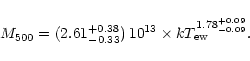
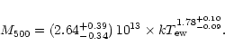
| entire sample | 1.78-0.09+0.09 | 2.61-0.33+0.38 |
| entire sample,
|
1.78-0.09+0.10 | 2.64-0.34+0.39 |
|
M>5 1013 |
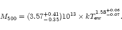
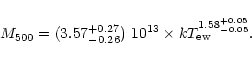
1.58-0.07+0.06 | 3.57-0.35+0.41 |
| 1.58-0.05+0.05 | 3.57-0.26+0.27 | |
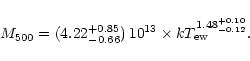
| Implying isothermality to sample with kT-profiles | ||
| entire sample | 1.89-0.09+0.10 | 2.45-0.32+0.37 |
|
M>5 1013 |
1.74-0.06+0.07 | 3.04-0.29+0.29 |
| 1.66-0.04+0.05 | 3.50-0.23+0.21 | |
The results, obtained for the flux-limited and the enlarged sample agree within the uncertainty of the fit. A correction for the observed redshift does not result in any change in the derived parameters. The derived slope of the M-T relation is steeper than the value of 1.5, expected from self-similar scaling relations. The normalization obtained in the hydrodynamical/N-body simulations of Evrard et al. (1996) is higher than found here. No break in the M-T relation is visible over the whole range of temperatures.
Note, however, that the determination of the mass value itself depends on the temperature, therefore some care has to be taken in the interpretation of the fit results. In the discussion, which follows below, we take this effect into account.
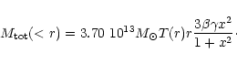
To derive the total masses for the clusters in this sample, we use the
spatially resolved temperature profiles found in ASCA measurements
(Markevitch et al. 1998; Finoguenov & Ponman 1999; Finoguenov et al. 2000, hereafter FDP, FAD; Finoguenov et al. 2001). The
sample totals 39 systems with temperatures from 0.7 keV to 10 keV. This
corresponds to a factor of 100 difference in total mass, determined at a
given overdensity. A major difference of this sample, compared to studies of
Horner et al. (1999) and Nevalainen et al. (2000), is an inclusion of 22
systems with temperatures spanning the range from 0.7 keV to 3.5 keV. This
sample is therefore well suited to study the possible break in the M-Trelation, suggested by Nevalainen et al. (2000).
![\begin{figure}
\includegraphics[width=13cm]{ms10339f1.ps}
\end{figure}](/articles/aa/full/2001/12/aa10339/img31.gif) |
Figure 1: M-T relation for the enlarged HIFLUGCS (filled circles indicate the data with solid line indicating the best-fit). For comparison, the fit to the M-T relation for the flux-limited HIFLUGCS is also shown (dot-dashed line). The dashed line shows the result of simulations by Evrard et al. (1996) |
| Open with DEXTER | |
![\begin{figure}
\includegraphics[width=13cm]{ms10339f2.ps}
\end{figure}](/articles/aa/full/2001/12/aa10339/img32.gif) |
Figure 2:
M-T relation (analog to Fig. 1) for the sample
with temperature profiles. Crosses represent the mass determinations using
ASCA temperature profiles and ROSAT surface brightness profile fitting. The
dotted line denotes the best fit using the total sample, while the solid
line denotes the best fit, when groups (
M500<5 1013 |
In calculating the total cluster masses we used polytropic indices to describe the temperature profiles, omitting the cluster core, where effects of cooling may be important. For the total mass estimates, we used the fits to the surface brightness profiles from ROSAT PSPC data on the outskirts of the clusters from Vikhlinin et al. (1999), FDP, FAD, Finoguenov et al. (2001), thus avoiding the cooling zone of the cluster. We estimate the uncertainty of surface brightness profile fitting on the mass estimation as 4%. The uncertainties in the total mass estimations are much larger and are due to the uncertainty in temperature estimates and temperature gradients.
There could be a systematic effect in the analysis of ROSAT surface
brightness profiles of groups, caused by variation of the ROSAT
countrate-to-emission measure conversion factor at low emission temperatures
(Böhringer 1996; Finoguenov et al. 1999). To evaluate this effect, we
compare our fits to ROSAT surface brightness profiles with the spectral
normalizations, derived in our 3d modeling of ASCA data. The latter accounts
for both temperature and metallicity effects, but has larger systematics due
to the complex PSF. From a good agreement, found in this comparison, a
possible systematics in the total mass calculation, resulting from our
approach to measuring the ![]() values, is constrained to be less than
10%.
values, is constrained to be less than
10%.
Under the assumption of hydrostatic equilibrium, when the density profile is
described by a ![]() -model and the temperature distribution is expressed
in polytropic form (
-model and the temperature distribution is expressed
in polytropic form (
![]() ), the total mass within
the radius
), the total mass within
the radius
![]() is simply
is simply
In calculating the emission-averaged temperatures we removed the effects of cooling flows and emission lines. Thus, these temperatures are not subject to effects discussed in Mathiesen & Evrard (2000, hereafter ME00). The deviation of the measured M-T relation relative to the simulated one could be characterized by observing a higher temperature for a given mass. If a distinction exists between the spectral temperature measurements and the mass-averaged temperatures, as discussed in ME00, the above-mentioned discrepancy should only increase. This, however, is not true in the case of decreasing temperature profiles. We will return to this issue below.
In this section we investigate how the resulting parameters describing the M-T relation depend on the selection of the sample, with the most important results listed in Table 1.
Without the correction for the observed redshift the fit to the M-Trelation using the bisector method by Akritas & Bershady (1996) gives
![\begin{figure}
\includegraphics[width=8.4cm,clip]{ms10339f3.ps}
\end{figure}](/articles/aa/full/2001/12/aa10339/img37.gif) |
Figure 3:
Parameters of the bisector fit to the M-T relation. Contours,
drawn at 1, 2 and 3 |
| Open with DEXTER | |
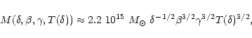
Our results on the slope of the M-T relation are in agreement with
findings of Nevalainen et al. (2000), who determined a significantly steeper
slope than 1.5 (
![]() ,
90% confidence interval is cited) at an
overdensity of 1000.
,
90% confidence interval is cited) at an
overdensity of 1000.
Horner et al. (1999) find a flatter M-T relation, consistent with a value of 1.5, but their sample lacks groups. Nevalainen et al. (2000) suggest on the basis of their comparison of the M-T relation, derived for hot clusters and adding a few groups, that there might be a break in the M-Trelation, occurring below 4 keV. Since our data uniquely sample a temperature range from groups to clusters of galaxies, we are in a position to check this suggestion.
The M-T relation derived without groups (
M500>5 1013 ![]() )
is
)
is
![\begin{figure}
\includegraphics[width=8.4cm,clip]{ms10339f4.ps}
\end{figure}](/articles/aa/full/2001/12/aa10339/img41.gif) |
Figure 4:
Parameters of the bisector fit to the M-T relation, derived
from the sample with temperature profiles. Light grey contours describe the
slope and normalization of the M-T relation for clusters with temperature
below 4 keV. In grey we show the fit to all the data and in black those
excluding the groups (
M500<5 1013 |
| Open with DEXTER | |
Restricting ourselves to the systems with temperatures above 3 keV, the fit
is

To study the confidence area of the parameter estimation for the above fits, we choose a normalization at 3.5 keV, which makes the determination of the slope less dependent on the normalization. We present the values derived this way in Fig. 4. It can be seen from this figure that the total sample is inconsistent with a power law index of 1.5 on more than 99.9% level. The high-temperature system sample (excluding groups), although revealing a flatter index consistent with a value of 1.5, is not strongly deviant from the total sample, e.g. the break in the M-T relation has only 95% confidence. A steeper slope, derived for the low-temperature end of the sample, can still be considered as a fluctuation. However, larger errors in the parameter determination in the case of inclusion of groups are due to the large spread of groups on the M-T relation (see Fig. 2). So, the meaning of ``fluctuation'' is that a subsample of systems leading to a derivation of the flat slope could be drawn from the existing sample at a high probability. The origin of the scatter is further discussed in Sect. 5.
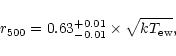
In many studies the virial radius is suggested as a unit of length (e.g. Evrard et al. 1996; Markevitch et al. 1998; Cen & Ostriker 1999) to provide a
comparison among the systems at equal overdensity. For these estimations,
the luminosity averaged temperature of the cluster is used (Markevitch et al.
1998, FDP). Therefore, we provide here a relation between r500 and the
luminosity-weighted X-ray temperature, derived from the data in Table 2:
| Name | z | kT | kT500 | M500 | r500 |
|
|
||
| keV | keV | 1014 |
Mpc | Mpc | Mpc | ||||
| A2029 | 0.077 |
|
|
|
|
0.68 | 0.28 |
|
2.82 |
| A401 | 0.074 |
|
|
|
|
0.63 | 0.27 |
|
1.82 |
| A3266 | 0.055 |
|
|
|
|
0.74 | 0.50 |
|
1.57 |
| A1795 | 0.062 |
|
|
|
|
0.83 | 0.39 |
|
1.56 |
| A2256 | 0.058 |
|
|
|
|
0.82 | 0.52 |
|
1.83 |
| A3571 | 0.040 |
|
|
|
|
0.69 | 0.27 |
|
2.28 |
| A1651 | 0.085 |
|
|
|
|
0.70 | 0.26 |
|
1.62 |
| A119 | 0.044 |
|
|
|
|
0.66 | 0.48 |
|
1.28 |
| A3558 | 0.048 |
|
|
|
|
0.55 | 0.19 |
|
1.39 |
| A2199 | 0.030 |
|
|
|
|
0.64 | 0.14 |
|
1.25 |
| A496 | 0.033 |
|
|
|
|
0.70 | 0.25 |
|
1.32 |
| A4059 | 0.048 |
|
|
|
|
0.67 | 0.22 |
|
0.92 |
| A3112 | 0.075 |
|
|
|
|
0.63 | 0.12 |
|
1.74 |
| Hydra | 0.057 |
|
|
|
|
0.66 | 0.12 |
|
1.35 |
| A2063 | 0.035 |
|
|
|
|
0.69 | 0.22 |
|
0.93 |
| MKW3S | 0.045 |
|
|
|
|
0.71 | 0.30 |
|
1.16 |
| A2657 | 0.040 |
|
|
|
|
0.76 | 0.37 |
|
1.17 |
| AWM7 | 0.017 |
|
|
|
|
0.53 | 0.10 |
|
0.75 |
| A2052 | 0.035 |
|
|
|
|
0.64 | 0.10 |
|
0.46 |
| HCG94 | 0.042 |
|
|
|
|
0.48 | 0.08 |
|
1.08 |
| 2A0335 | 0.035 |
|
|
|
|
0.65 | 0.08 |
|
0.92 |
| A4038 | 0.028 |
|
|
|
|
0.61 | 0.16 |
|
0.38 |
| A1060 | 0.011 |
|
|
|
|
0.70 | 0.16 |
|
0.31 |
| A2634 | 0.031 |
|
|
|
|
0.69 | 0.45 |
|
0.83 |
| MKW9 | 0.040 |
|
|
|
|
0.52 | 0.05 |
|
0.71 |
| AWM4 | 0.032 |
|
|
|
|
0.62 | 0.11 |
|
0.46 |
| A539 | 0.029 |
|
|
|
|
0.69 | 0.25 |
|
0.72 |
| MKW4S | 0.028 |
|
|
|
|
0.51 | 0.12 |
|
0.75 |
| A262 | 0.016 |
|
|
|
|
0.46 | 0.06 |
|
0.44 |
| A400 | 0.024 |
|
|
|
|
0.56 | 0.18 |
|
0.64 |
| N3258 | 0.009 |
|
|
|
|
0.34 | 0.05 |
|
0.57 |
| MKW4 | 0.020 |
|
|
|
|
0.64 | 0.18 |
|
0.66 |
| N6329 | 0.028 |
|
|
|
|
0.53 | 0.12 |
|
0.64 |
| HCG51 | 0.026 |
|
|
|
|
0.30 | 0.08 |
|
0.69 |
| N5044 | 0.009 |
|
|
|
|
0.51 | 0.01 |
|
0.28 |
| HCG62 | 0.014 |
|
|
|
|
0.31 | 0.02 |
|
0.58 |
| N4325 | 0.026 |
|
|
|
|
0.59 | 0.01 |
|
0.60 |
| IC4296 | 0.013 |
|
|
|
|
0.31 | 0.06 |
|
0.32 |
| N5129 | 0.023 |
|
|
|
|
0.60 | 0.10 |
|
0.58 |
As given in Eq. (1), the deduced mass depends on the temperature and
the parameters ![]() and
and ![]() ,
describing the shape of the density and
temperature profile. To further elucidate the origin of the behavior of the
M-T relation and to circumvent the direct dependence of M on T we
examine in Fig. 5 the dependence of
,
describing the shape of the density and
temperature profile. To further elucidate the origin of the behavior of the
M-T relation and to circumvent the direct dependence of M on T we
examine in Fig. 5 the dependence of ![]() (correctly
(correctly
![]() at r500) on T. We note four systems with
at r500) on T. We note four systems with
![]() that imply a steep dependence of beta on the temperature. They are mainly
responsible for the steep slope of the M-T relation in our sample with
spatially resolved temperatures. In fact, excluding these systems (IC 4296,
HCG62, HCG51, NGC 3258), but leaving other groups in, the M-T relation is
given by
that imply a steep dependence of beta on the temperature. They are mainly
responsible for the steep slope of the M-T relation in our sample with
spatially resolved temperatures. In fact, excluding these systems (IC 4296,
HCG62, HCG51, NGC 3258), but leaving other groups in, the M-T relation is
given by
![\begin{figure}
\includegraphics[width=7.8cm,clip]{ms10339f5.ps}
\end{figure}](/articles/aa/full/2001/12/aa10339/img242.gif) |
Figure 5:
Relation between density gradient (defined by
|
| Open with DEXTER | |
Horner et al. (1999) have found that the dependence of ![]() on
on
![]() is
responsible for the steepening of the derived M-T in the isothermal
assumption, but when the temperature profiles are taken into account, the
slope becomes 3/2 again. To verify this, we rewrite Eq. (1) in terms
of overdensity
is
responsible for the steepening of the derived M-T in the isothermal
assumption, but when the temperature profiles are taken into account, the
slope becomes 3/2 again. To verify this, we rewrite Eq. (1) in terms
of overdensity
As is seen from Figs. 6 and 7, the data show two
trends, which cancel each other: both very hot and very cold systems seem
to have stronger temperature gradients. So, the trend on the high-energy
part counterbalances the weak dependence of ![]() on T, while the trend
in the low-temperature part only reinforces the trend observed in
on T, while the trend
in the low-temperature part only reinforces the trend observed in
![]() .
Thus, it becomes clear why inclusion of groups makes such a drastic
difference in the derived M-T relation. An overall fit to these figures
gives
.
Thus, it becomes clear why inclusion of groups makes such a drastic
difference in the derived M-T relation. An overall fit to these figures
gives
![]() and
and
![]() .
.
![\begin{figure}
\includegraphics[width=7.8cm,clip]{ms10339f6.ps}
\end{figure}](/articles/aa/full/2001/12/aa10339/img251.gif) |
Figure 6:
Relation between |
| Open with DEXTER | |
![\begin{figure}
\includegraphics[width=7.8cm,clip]{ms10339f7.ps}
\end{figure}](/articles/aa/full/2001/12/aa10339/img252.gif) |
Figure 7:
Relation between
|
| Open with DEXTER | |
In fact, the arguments presented in Horner et al. (1999) are not strictly correct. They base their conclusion on the fact that
![]() for an individual cluster, where
for an individual cluster, where ![]() is the mass estimate using the
is the mass estimate using the ![]() -model and assuming isothermality and
-model and assuming isothermality and
![]() is the true mass of the cluster.
is the true mass of the cluster.
However, what is relevant is:
![]() for the cluster sample,
for the cluster sample,
![]() where
where
![]() is the
cluster core radius and
is the
cluster core radius and ![]() is the radius of overdensity
is the radius of overdensity ![]() ,
,
from which it follows:
![]()
This means that if clusters are self similar, the overestimate of the beta model is the same for all clusters. In view of this consideration, we note that there is a very close agreement between the parameters of the M-Trelation determined in our two samples. This agreement, which demonstrates that usage of the isothermality assumption does not bias the derived parameters of the M-T relation, can be used to justify the validity of the M-T relation, derived for high-redshift samples, where detailed temperature measurements are difficult and an assumption of isothermality is the only choice.
Following a suggestion of the referee, we examine also the effect of
assuming isothermality in deriving the total mass for the sample with
spatially resolved temperature measurements. The results are listed in Table
1. The slope of the M-T relation, obtained for the total
sample, is still steeper, while avoiding the systems with flat ![]() gives
results consistent with HIFLUGCS in both slope and normalization. We note that
the lowest
gives
results consistent with HIFLUGCS in both slope and normalization. We note that
the lowest ![]() value for the HIFLUGCS sample is 0.44, which again supports
the idea of the importance of the selection of the systems with respect to
their values of
value for the HIFLUGCS sample is 0.44, which again supports
the idea of the importance of the selection of the systems with respect to
their values of ![]() .
.
Concluding this section, we identify the inclusion of systems with low
values of ![]() as the most important cause of the steep slope of the
M-T relation, which could be overcome by excluding such systems from the
sample. As we have shown, a flat
as the most important cause of the steep slope of the
M-T relation, which could be overcome by excluding such systems from the
sample. As we have shown, a flat ![]() is not necessarily a unique
characteristic of groups, which most likely implies a different importance
of preheating in low-mass systems. This is in qualitative agreement with the
preferential infall scenario, proposed by FAD.
is not necessarily a unique
characteristic of groups, which most likely implies a different importance
of preheating in low-mass systems. This is in qualitative agreement with the
preferential infall scenario, proposed by FAD.
In all the fits, however, the normalization of the M-T relation appears
smaller than in the simulations of Evrard et al. (1996). In the following, we
would like to comment on this issue. As pointed out by Nevalainen et al.
(2000), the resolution in the simulations of Evrard et al. (1996) is
insufficient to resolve the cluster cores. One can assume, however, that
their simulations are correct at low overdensities. Since we measure the
temperature up to the radius of the overdensity chosen for the mass
calculations, we can directly check this effect by using a temperature at
the radius of mass determination, (T500), instead of the
luminosity-weighted temperatures. Such a comparison may also be less
affected by preheating, since at
![]() no significant variation in
the gas fraction is seen (Ettori & Fabian 1999; Vikhlinin et al.
1999). Taking measured temperatures also avoids many possible effects of averaging, discussed in ME00 and is
therefore closer to the relations predicted for the mass-weighted
temperature. A fit to the
M500-T500 relation reads as
no significant variation in
the gas fraction is seen (Ettori & Fabian 1999; Vikhlinin et al.
1999). Taking measured temperatures also avoids many possible effects of averaging, discussed in ME00 and is
therefore closer to the relations predicted for the mass-weighted
temperature. A fit to the
M500-T500 relation reads as
The normalization of M-T500 in the simulations by Evrard et al. (1996)
is about
9.-15. 1013 ![]() (considering
(considering
![]() ),
closer to the observed points, but still in obvious disagreement (fixing the
slope to 1.5 we obtain a normalization at 1 keV of
4.81-0.29+0.30 1013
),
closer to the observed points, but still in obvious disagreement (fixing the
slope to 1.5 we obtain a normalization at 1 keV of
4.81-0.29+0.30 1013 ![]() ).
).
![\begin{figure}
\includegraphics[width=8.2cm,clip]{ms10339f8.ps}
\end{figure}](/articles/aa/full/2001/12/aa10339/img263.gif) |
Figure 8: M500-T500 relation. Dashed line shows the rescaled simulations by Evrard et al. (1996) |
| Open with DEXTER | |
Comparison between the X-ray and the virial mass measurements, obtained using velocity dispersions, is long known to be subject to contradictions, with velocity bias considered as the most likely origin. Recently, a new compilation of optical measurements was made by Girardi et al. (1998), where a much more detailed study was carried out, e.g. different velocity dispersion profiles in clusters were identified. Since we have measured the masses for many clusters in common, we can combine the X-ray mass with velocity dispersion measurements to provide a comparison with high-resolution dark matter simulations.
We take high-resolution
![]() (
(
![]() ,
,
![]() ;
H0=70 km s-1 Mpc-1) simulations using the
ART code (Kravtsov et al. 1997), with 2563 particles of
1.1 109
;
H0=70 km s-1 Mpc-1) simulations using the
ART code (Kravtsov et al. 1997), with 2563 particles of
1.1 109 ![]() each in a simulation box of 60h-1 Mpc (see
Gottloeber et al. 1999 for details). The particular runs of the ART code we
use for comparison are characterized by a scale of velocity dispersion with
overdensity of
each in a simulation box of 60h-1 Mpc (see
Gottloeber et al. 1999 for details). The particular runs of the ART code we
use for comparison are characterized by a scale of velocity dispersion with
overdensity of
![]() with a residual scatter around
the best-fit of 20-30%. Within the simulated box, 17 clusters have been
identified and we build the
with a residual scatter around
the best-fit of 20-30%. Within the simulated box, 17 clusters have been
identified and we build the
![]() relation, scaling the measurements
done at different overdensities. One possible weakness of such a comparison
is that in the simulations we have studied the dispersion of the dark
matter, not of the galaxies.
relation, scaling the measurements
done at different overdensities. One possible weakness of such a comparison
is that in the simulations we have studied the dispersion of the dark
matter, not of the galaxies.
![\begin{figure}
\includegraphics[width=8cm,clip]{ms10339f9.ps}
\end{figure}](/articles/aa/full/2001/12/aa10339/img268.gif) |
Figure 9:
|
| Open with DEXTER | |
Optical observations reveal 3 types of clusters, according to their degree of virialization. In comparing the data, we have scaled the optical velocity dispersions according to the given type of cluster, using identification and scaling profiles, reported in Girardi et al. (1998). To compare our X-ray results with the work of Girardi et al. (1998), we rescale our mass estimates to the overdensity of 90, using the Navarro et al. (1996) profile.
The resulting
![]() relation is presented in Fig. 9. The
outliers on the
relation is presented in Fig. 9. The
outliers on the
![]() relation, A2319, A3558 and A400, are already
known to have a peculiar structure (Feretti et al. 1997;
Venturi et al. 2000; Lloyd-Davies et al. 2000). The scatter of the
other points around the simulations is within 30% and therefore comparable
to the scatter seen in simulations. We note, however, that there is a trend
of type B and C clusters to have a higher velocity dispersion for a given
mass, which is consistent with a definition of their type: type B and C are
older systems, according to modeling of Girardi et al. (1998), that should
imply a higher formation redshift. Since such a correction is not introduced
into the virial mass calculation, this results in a slight bias in mass
estimates for these clusters, as seen in Fig. 10.
relation, A2319, A3558 and A400, are already
known to have a peculiar structure (Feretti et al. 1997;
Venturi et al. 2000; Lloyd-Davies et al. 2000). The scatter of the
other points around the simulations is within 30% and therefore comparable
to the scatter seen in simulations. We note, however, that there is a trend
of type B and C clusters to have a higher velocity dispersion for a given
mass, which is consistent with a definition of their type: type B and C are
older systems, according to modeling of Girardi et al. (1998), that should
imply a higher formation redshift. Since such a correction is not introduced
into the virial mass calculation, this results in a slight bias in mass
estimates for these clusters, as seen in Fig. 10.
![\begin{figure}
\includegraphics[width=8cm,clip]{ms10339f10.ps}
\end{figure}](/articles/aa/full/2001/12/aa10339/img269.gif) |
Figure 10: Comparison of the X-ray and optical mass estimates. Black crosses denote type A clusters in Girardi et al. (1998), grey crosses type B and light grey crosses type C. Type A clusters show the best agreement with the X-ray mass measurements |
| Open with DEXTER | |
The issue of the redshift of cluster formation was strongly suggested in studies of Lilje (1992); Kitayama & Suto (1996); Voit & Donahue (1998). The effect on the M-T relation is such that for a given mass, the systems that formed at earlier times should have higher temperatures. Since this scenario is in qualitative agreement with trends observed by comparing our sample with the simulations of Evrard et al. (1996), we decided to estimate whether the shift observed in the M-T relation could be explained just by this scenario.
To do this, we invert the problem, i.e. use the X-ray mass and temperature
measurements and the M-T relation obtained in the simulations to derive
the distribution of redshifts of cluster formation for our sample. In more
detail, for a measured mass of the system, we compare the measured
temperature with the value obtained from the simulation for the measured
mass and attribute the difference to the redshift of cluster formation,
which for
![]() is simply
is simply
![]() .
To be able to do this, one should
make sure that the simulated relation explicitly assumes that the clusters
form at the redshift of observation. Fortunately, the simulations of Evrard
et al. (1996) have this assumption, which is quite logical for
.
To be able to do this, one should
make sure that the simulated relation explicitly assumes that the clusters
form at the redshift of observation. Fortunately, the simulations of Evrard
et al. (1996) have this assumption, which is quite logical for
![]() ,
used for most of their runs (Metzler, private communication).
,
used for most of their runs (Metzler, private communication).
In Fig. 11 we illustrate the effect of the redshift of cluster
formation, by comparison with the model of Lacey & Cole (1993) following
the formulae presented in Balogh et al. (1999) for
![]() .
We
subdivide our sample into 3 parts with masses in the 0.1-0.8, 0.8-3 and
3-15 1014
.
We
subdivide our sample into 3 parts with masses in the 0.1-0.8, 0.8-3 and
3-15 1014 ![]() range. From the figure one can see that the
theoretical prediction varies significantly between the three subsets and
generally matches the trends seen in the corresponding subset. While a more
detailed comparison should await an M-T relation simulated with much
better resolution, we can state already that a steeper slope of the observed
M-T relation implies that lower-mass systems form preferentially at
earlier times, compared to rich clusters. The formation redshift
distribution for groups is wider than the model prediction, which can be
taken as a sign of the importance of SN preheating, but a more detailed
study is needed to verify this suggestion.
range. From the figure one can see that the
theoretical prediction varies significantly between the three subsets and
generally matches the trends seen in the corresponding subset. While a more
detailed comparison should await an M-T relation simulated with much
better resolution, we can state already that a steeper slope of the observed
M-T relation implies that lower-mass systems form preferentially at
earlier times, compared to rich clusters. The formation redshift
distribution for groups is wider than the model prediction, which can be
taken as a sign of the importance of SN preheating, but a more detailed
study is needed to verify this suggestion.
![\begin{figure}
\includegraphics[width=7.8cm,clip]{ms10339f11.ps}
\end{figure}](/articles/aa/full/2001/12/aa10339/img271.gif) |
Figure 11:
Redshifts of cluster formation, deduced from a requirement for
measurements to match the simulations of Evrard et al. (1996). The black
solid histogram shows the calculation for the sample with temperature
profiles with dashed histograms indicating the number count errors at the 68%
confidence level. We present the comparison with the model of Lacey & Cole
(1993) following the formulae presented in Balogh et al. (1999) for
|
| Open with DEXTER | |
We can already identify one source of bias in the formation redshift
distribution of the clusters in the present study. Systems that collapsed
recently bear indications of recent merger activity and therefore are
selectively removed from the sample aimed to determine the mass using the
assumption of hydrostatic equilibrium. Therefore, the first bin in the
derived ![]() distribution should be disregarded in
Fig. 11. Flux-limited samples, such as HIFLUGCS, are in principle also
biased in this regard, since older systems are expected to be brighter for a
given mass. The lack of clusters lying close to the simulations on the
M-T plane is also caused by influence of a central region on the
determination of the luminosity averaged temperature, since formation of the
central part of a cluster is slightly shifted towards higher formation
epochs.
distribution should be disregarded in
Fig. 11. Flux-limited samples, such as HIFLUGCS, are in principle also
biased in this regard, since older systems are expected to be brighter for a
given mass. The lack of clusters lying close to the simulations on the
M-T plane is also caused by influence of a central region on the
determination of the luminosity averaged temperature, since formation of the
central part of a cluster is slightly shifted towards higher formation
epochs.
We have studied the M-T relation using a sample of clusters with resolved temperature profiles and also using HIFLUGCS. Our findings are
Acknowledgements
The authors thank Stephan Gottloeber for providing the results of simulations using ART code. AF acknowledges useful conversations with Monique Arnaud, Stefano Ettori, Yasushi Ikebe, Maxim Markevitch, Chris Metzler, Volker Mueller and Alexey Vikhlinin during preparation of this paper. AF acknowledges support from Alexander von Humboldt Stiftung and NASA grant NAG5-3064 during preparation of this work. The authors thank the anonymous referee for useful comments on the manuscript. The authors acknowledge the devoted work of the ROSAT and ASCA operation and calibration teams, without which this paper would not be possible.