A&A 367, 840-847 (2001)
DOI: 10.1051/0004-6361:20000493
A photometric study of the W UMa-type system U Pegasi
G. Djurasevic1 - H. Rovithis-Livaniou2 - P. Rovithis3 -
S. Erkapic1 - N. Milovanovic1
1 - Astronomical Observatory, Volgina 7, 11050 Belgrade, Yugoslavia
2 - Section of Astrophysics-Astronomy & Mechanics, Dept. of Physics,
Athens University, GR Zografos 157 84, Athens, Greece
3 -
Astron. Institute, National Observatory of Athens, PO Box 20048, 118 10 Athens, Greece
Received 14 April 2000 / Accepted 20 November 2000
Abstract
In the present study, the activity of the eclipsing binary of the W UMa-type
system U Peg is examined by analysing the photoelectric observations covering
the period from 1950 to 1989. During this period, the light curves show
significant differences and asymmetries. The analysis of the corresponding
light curves is made using Djurasevic's inverse problem method.
To explain the light-curve asymmetries and variations, we used a Roche model
that involved regions containing spots on the components. The analysis shows that
the system U Peg is in an overcontact configuration
(
 ). The Roche model
with spotted areas on the cooler component yields a good fit of the
observations for the whole set of the analysed light curves without any
changes of the basic system parameters. This indicates that
the complex nature of the light-curve variations during the examined period
can be explained by the evolution and motion of spotted
areas on the cooler component. According to the obtained results, the spotted
areas cover a significant part of
the stellar surface; the changes in their location and size with time are
examined.
). The Roche model
with spotted areas on the cooler component yields a good fit of the
observations for the whole set of the analysed light curves without any
changes of the basic system parameters. This indicates that
the complex nature of the light-curve variations during the examined period
can be explained by the evolution and motion of spotted
areas on the cooler component. According to the obtained results, the spotted
areas cover a significant part of
the stellar surface; the changes in their location and size with time are
examined.
Key words: stars: individual: U Peg - binaries: close: starspots - stars:
activity
The variability of U Peg (
 )
was discovered by Chandler
(1895) and the system belongs to the W sub-class of the W UMa-type
eclipsing binaries. From photoelectric observations it was found that its
light curves are variable.
)
was discovered by Chandler
(1895) and the system belongs to the W sub-class of the W UMa-type
eclipsing binaries. From photoelectric observations it was found that its
light curves are variable.
Regarding the spectral type of U Peg, Adams et al. (1924) classified it
as F3, but later this was revised to G3 (Adams et al.
1935). Struve et al. (1950) estimated the radial velocities
of the two components from 4 spectra of the system, but the
most recent and most accurate radial velocity observations were made by
Lu (1985).
Some of the light curves of the system have been analysed previously by
different methods; e.g. using the classical Russell model (Binnendijk
1960), Kopal's frequency domain techniques (Lafta et al. 1986) or W-D code (Russo et al. 1982; Zhai et al.
1984; Zhai et al. 1988). In the present paper,
photoelectric observations (La Fara 1952; Binnendijk
1960; Rigterink 1972; Zhai et al. 1984
and Maupomé et al. 1991) of U Peg were analysed
to study the activity of the system and to estimate the orbital and
physical parameters of U Peg.
To analyse these asymmetric light curves, probably deformed by the presence
of spotted areas on the components, we used Djurasevic's
(1992a) programme
generalised to the case of an overcontact configuration (Djurasevic et al. 1998). The programme is based on the Roche model and the
principles arising from the paper by Wilson & Devinney (1971). The
light-curve analysis was made by applying the inverse-problem method
(Djurasevic 1992b) based on Marquardt's
(1963) algorithm.
According to this method, the stellar size in the model is described
by the filling factors for the critical Roche lobes F1,2 of
the primary and secondary component, respectively, which tell us to what
degree the stars in the system fill their corresponding critical
lobes. For synchronous rotation of the components these factors
are expressed as the ratio of the stellar polar radii, R1,2,
and the corresponding polar radii of the critical Roche lobes, i.e.,
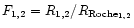 .
In the case of an overcontact
configuration the potential
.
In the case of an overcontact
configuration the potential
 characterising the common
photosphere is derived with the filling factor of the critical
Roche lobe F1>1 of the primary, while the factor F2 may be
excluded from further consideration. The degree of overcontact is defined
in the classical way (Lucy & Wilson 1979) as:
characterising the common
photosphere is derived with the filling factor of the critical
Roche lobe F1>1 of the primary, while the factor F2 may be
excluded from further consideration. The degree of overcontact is defined
in the classical way (Lucy & Wilson 1979) as:
![\begin{eqnarray*}f{\rm _{over}[\%]=100\cdot(\Omega_{1,2}-\Omega_i)/(\Omega_o-\Omega_i)},
\end{eqnarray*}](/articles/aa/full/2001/09/aa9840/img5.gif)
where
,
 ,
and
,
and
 are the potentials of
the common photosphere and of the inner and outer contact surfaces,
respectively.
To achieve more reliable estimates of the model parameters in the
light-curve analysis programme, we applied a quite dense coordinate grid, having
are the potentials of
the common photosphere and of the inner and outer contact surfaces,
respectively.
To achieve more reliable estimates of the model parameters in the
light-curve analysis programme, we applied a quite dense coordinate grid, having
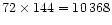 elementary cells per star. The intensity and angular
distribution of radiation of elementary cells are determined by the stellar
effective temperature, limb-darkening, gravity-darkening and by the effect of
reflection in the system.
elementary cells per star. The intensity and angular
distribution of radiation of elementary cells are determined by the stellar
effective temperature, limb-darkening, gravity-darkening and by the effect of
reflection in the system.
The presence of spotted areas (dark or bright) enables us to explain the
asymmetries and the light-curve anomalies. In our code these active regions
are approximated by circular spots,
characterised by the temperature contrast of the spot with respect to the
surrounding photosphere (
 ), by the angular dimension (radius)
of the spot (
), by the angular dimension (radius)
of the spot (
 )
and by the longitude (
)
and by the longitude (
 )
and latitude
(
)
and latitude
(
 )
of the spot centre. The longitude (
)
is measured
clockwise (as viewed from the direction of the +Z-axis) from the +X-axis
(line connecting star centres) in the range
)
of the spot centre. The longitude (
)
is measured
clockwise (as viewed from the direction of the +Z-axis) from the +X-axis
(line connecting star centres) in the range  -
- .
The latitude
(
)
is measured from
at the stellar equator (orbital plane)
to
.
The latitude
(
)
is measured from
at the stellar equator (orbital plane)
to  towards the "north'' (+Z)
and
towards the "north'' (+Z)
and  towards the "south'' (-Z)
pole.
towards the "south'' (-Z)
pole.
For a successful application of this model in the analysis
of the observed light curves, the method proposed by Djurasevic
(1992b) was used. Optimum model parameters are
obtained through the
minimization of
 ,
where
,
where
 is the residual between the
observed (LCO) and synthetic (LCC) light curves for a given orbital
phase. The minimization of S is done in an iterative cycle of corrections of
the model parameters. In this way the inverse-problem method gives us the
estimates of system parameters and their standard errors.
is the residual between the
observed (LCO) and synthetic (LCC) light curves for a given orbital
phase. The minimization of S is done in an iterative cycle of corrections of
the model parameters. In this way the inverse-problem method gives us the
estimates of system parameters and their standard errors.
In the analysis of the light curves, instead of the often used and somewhat
questionable practice of forming normal points, we used the original
observational data in order to avoid negative influences of such
normalization. La Fara's (1952) observations are an
exception because only the normal points published by the
author were available to us.
The present light-curve analysis shows that during the deeper (primary) minimum
the cooler (more-massive and larger) component eclipses the hotter
(less-massive and smaller) one. Since the primary minimum is an occultation,
the mass-ratio of the components was fixed in the inverse problem
at Zhai et al.'s (1988) simultaneous (photometric and radial
velocity) solution
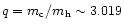 .
Based on the spectral type (G2 V;
Zhai et al. 1988) the temperature of the less-massive (hotter)
component,
.
Based on the spectral type (G2 V;
Zhai et al. 1988) the temperature of the less-massive (hotter)
component,
 ,
was set at 5800 K. The indexes (h, c) refer to the
hotter (less-massive) and cooler (more-massive) components respectively.
,
was set at 5800 K. The indexes (h, c) refer to the
hotter (less-massive) and cooler (more-massive) components respectively.
The values of the limb-darkening coefficients were derived from the
stellar effective temperature and surface gravity, according to the given
spectral type, by using the polynomial proposed by Díaz-Cordovés et al.
(1995). During the process of optimisation, according to the temperature
changes, we have an automatic recomputation of the limb-darkening. Following
Lucy (1967), Rucinski (1969) and Rafert & Twigg
(1980), the gravity-darkening coefficients of the stars,
 ,
and their albedos,
,
and their albedos,
 ,
were set at the values of
0.08 and 0.5, respectively, appropriate for stars with convective envelopes.
,
were set at the values of
0.08 and 0.5, respectively, appropriate for stars with convective envelopes.
The present analysis yields
 for the filling coefficient in the
critical Roche lobe, i.e., the overcontact configuration. Tidal effects
are expected to contribute to synchronisation of the rotational and
orbital periods. Therefore, in the inverse problem we adopted
for the filling coefficient in the
critical Roche lobe, i.e., the overcontact configuration. Tidal effects
are expected to contribute to synchronisation of the rotational and
orbital periods. Therefore, in the inverse problem we adopted
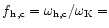 1.0 for nonsynchronous rotation
coefficients, where
1.0 for nonsynchronous rotation
coefficients, where
 is the ratio of the angular rotation
rate (
is the ratio of the angular rotation
rate (
 )
to the Keplerian (
)
to the Keplerian (
 )
orbital revolution rate.
)
orbital revolution rate.
In previous versions of our programme, there were two different
possibilities in the application of the model with respect to the
treatment of the radiation law: the simple black-body theory, or the
stellar atmosphere models by Carbon & Gingerich (1969) (CG). Our
current version of the programme for the light-curve analysis employs the
new promising Basel Stellar Library (BaSeL). We have explored the
"corrected''
BaSeL model flux distributions, consistent with extant
empirical calibrations (Lejeune et al. 1997, 1998),
and with a large range of effective temperatures
 ,
surface gravities,
,
surface gravities,
 and metallicity,
![${\rm -1\le[Fe/H]\le 1}$](/articles/aa/full/2001/09/aa9840/img30.gif) ,
where [Fe/H] is the logarithmic
metal abundance. The surface gravities can be
derived very accurately from the masses and radii of close binary (CB)
stars by solving the inverse problem of the light-curve analysis, but
the temperature determination is related to the assumed metallicity and
strongly depends on photometric calibration.
,
where [Fe/H] is the logarithmic
metal abundance. The surface gravities can be
derived very accurately from the masses and radii of close binary (CB)
stars by solving the inverse problem of the light-curve analysis, but
the temperature determination is related to the assumed metallicity and
strongly depends on photometric calibration.
In the inverse problem, the fluxes are calculated in each iteration for
the current values of temperatures and
 by
interpolation in both of these quantities in the atmosphere tables, as an
input, for a given metallicity
of the CB components. The metallicity of the involved CB components can be
different. It is because of this that we can use individual, different tables
as an input
for each star, and in this way choose the best calculations for its
particular atmospheric parameters. Compared to Vaz et al. (1995), our
two-dimensional flux interpolation in
by
interpolation in both of these quantities in the atmosphere tables, as an
input, for a given metallicity
of the CB components. The metallicity of the involved CB components can be
different. It is because of this that we can use individual, different tables
as an input
for each star, and in this way choose the best calculations for its
particular atmospheric parameters. Compared to Vaz et al. (1995), our
two-dimensional flux interpolation in
 and
is
based on the application of the bicubic spline interpolation
(Press et al. 1992). This proved to be a good choice.
and
is
based on the application of the bicubic spline interpolation
(Press et al. 1992). This proved to be a good choice.
By choosing and fixing the particular input switch, the programme for the
light-curve analysis can be simply redirected to the Planck or CG
approximation, or to the more realistic BaSeL model atmospheres. Disagreement
between individual B and V solutions decreases if we introduce the
"corrected'' BaSeL model flux distributions. A change in
the assumed metallicity causes a noticable change in the predicted stellar
effective temperature. The value of the chemical abundance of the
components was obtained by checking several different values around solar
metallicity. In the case of U Peg, the best fit of the B
and V light curves was obtained with
![${\rm [Fe/H]_{h,c}=0.2}$](/articles/aa/full/2001/09/aa9840/img33.gif) for the metallicity of
the components. With this value, the individual B and V
solutions are in good agreement. The results presented here
are given within this stellar atmosphere approximation.
for the metallicity of
the components. With this value, the individual B and V
solutions are in good agreement. The results presented here
are given within this stellar atmosphere approximation.
Among the light curves that were analysed, Zhai et al.'s (1984)
photoelectric BV light curves were the most symmetrical.
For the estimation of the system's basic parameters we used the 1958 Binnendijk
light curves (1960). In these light curves, the system is brighter
in the maximum after a primary minimum than in the rest of the analysed light
curves.
This checking was done in a relative way, by measuring the light curve
amplitude (max-min), and also by comparing the light levels in the light
curve maxima. By that we have in mind that Binnendijk's observations were made
with a non-standard filter combination, whose effective wavelengths were
 (V-filter) and
 (B-filter). The problem exists also for La Fara's
(1952) observations, which were
made with pre-Johnson filters, with effective wavelengths
(B-filter). The problem exists also for La Fara's
(1952) observations, which were
made with pre-Johnson filters, with effective wavelengths
 (V-filter) and
 (B-filter).
Other observations are in Johnson's system. The differences of effective
wavelengths of La Fara's and Binnendijk's filters from Johnson's filters
have as a consequence a wavelength-dependent influence on the light curve
amplitude. This influence can be estimated and for both groups of observations
lies in the interval
(B-filter).
Other observations are in Johnson's system. The differences of effective
wavelengths of La Fara's and Binnendijk's filters from Johnson's filters
have as a consequence a wavelength-dependent influence on the light curve
amplitude. This influence can be estimated and for both groups of observations
lies in the interval
 (
(
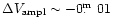 ;
;
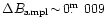 - Binendijk's observations and

 ;
;

 - La Fara's
observations).
The obtained solutions show that Binnendijk's 1958 light level, at
orbital phase 0.25 is very probably free of spot effects. In the analysis of
these light curves, the inclination of the orbit was estimated to be
- La Fara's
observations).
The obtained solutions show that Binnendijk's 1958 light level, at
orbital phase 0.25 is very probably free of spot effects. In the analysis of
these light curves, the inclination of the orbit was estimated to be
 ,
the filling coefficient for the critical Roche lobe
,
the filling coefficient for the critical Roche lobe
 and the
temperature of the cooler (more massive) star
and the
temperature of the cooler (more massive) star
 .
.
Since the stars in the system have external convective envelopes, which can
exhibit magnetic activity, we started the "spotted solution'' by assuming that
the components of U Peg have cool spots, of the same nature as solar
magnetic spots. Moreover, since the results of the light-curve analysis
depend on the choice of the adopted working hypothesis, the analysis was
carried out within the framework of several hypotheses with spotted
areas on the components.
We rejected those hypotheses which produced significantly different
values of the parameters for the system and the active spotted areas,
estimated by analysing the individual light curves in the B and Vpassbands. Finally we chose the Roche model with dark spotted areas on the
more massive (cooler) component as the optimum solution. Within
this hypothesis the analysis of the light curves yields mutually
consistent parameters of the system and active region in the B and Vpassbands. In this case we obtained a very good fit of the observations for
the whole set of analysed light curves without any
changes in the system's basic parameters. Consequently, the presence of
dark spotted areas on the cooler star can be taken as possible.
The system's basic parameters, obtained by analysing Binnendijk's
(1960) light curves, were fixed in the inverse-problem solution
for other, more or less deformed and asymmetrical light curves. In the
subsequent analysis, these light curves are normalised to the reference light
level of the 1958 Binnendijk light curves at orbital phase 0.25, and
their analysis was made with optimisation in the spot parameters.
The results indicate that the complex nature of the light-curve
variations during the examined period can be explained by changes
in the parameters of the spotted areas.
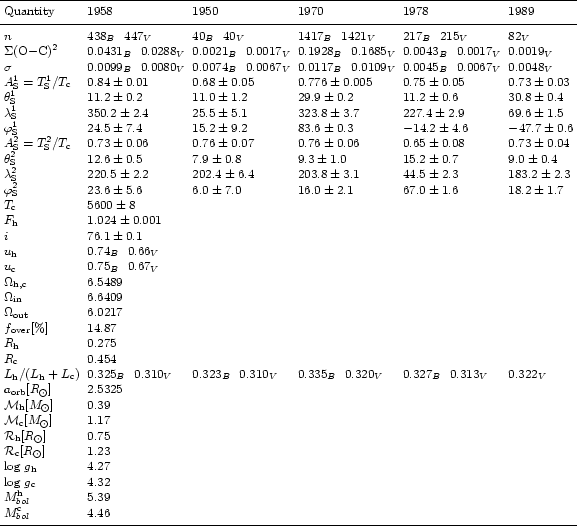
The parameters derived from the light-curve analysis are listed in
Table 1. The errors of the parameter estimates arise from the
nonlinear least-squares method, on which the inverse-problem method is based.
The first three rows of the table present the number of observations
n, the final sum of squares of residuals between observed (LCO) and synthetic
(LCC) light curves
and the standard deviation of the observations
In Table 1, the indices (B,V) denote the B and V-filter
observations, respectively.
In the same table the spot characteristics (spot temperature factor,
;
longitude,
;
latitude,
;
angular radius,
)
are also given. Determination of these parameters
is based on a simultaneous fitting of the available light curves in the B and V
photometric bands for the different epochs of the observations with the same set
of basic system parameters.
Finally, in Table 1 we present some important absolute parameters.
They are derived from the mass-ratio of the components
(
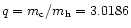 ), orbital period (
 )
and the semimajor
orbital axis (
)
and the semimajor
orbital axis (
![$a_{\rm orb} [R_{\odot}]=2.5325$](/articles/aa/full/2001/09/aa9840/img52.gif) )
estimated by Zhai et al.
(1988) on the basis of the simultaneous solution of the light
(Zhai et al. 1984) and radial velocity (Lu 1985) curves.
)
estimated by Zhai et al.
(1988) on the basis of the simultaneous solution of the light
(Zhai et al. 1984) and radial velocity (Lu 1985) curves.
Based on the Hipparcos parallax, Rucinski & Duerbeck (1997)
derived for the absolute visual magnitude of the system
 .
From our data in Table 1, including the
bolometric corrections, we derived for the absolute visual magnitude of
the system
.
From our data in Table 1, including the
bolometric corrections, we derived for the absolute visual magnitude of
the system
 .
In the limits of the error this value agrees with the
absolute visual magnitude of the system based on the Hipparcos parallax.
.
In the limits of the error this value agrees with the
absolute visual magnitude of the system based on the Hipparcos parallax.
Table 1:
Results of the analysis of the U Peg (1950, 1958, 1970, 1978, 1989)
photometrical observations obtained by solving the light curve inversion
problem for the Roche model with spotted areas on the more-massive (cooler)
component
 |
|
FIXED PARAMETERS: |
| Open with DEXTER |
 K - temperature of the less-massive (hotter) component. K - temperature of the less-massive (hotter) component.
|
 K - temperature of the more-massive (cooler) star. K - temperature of the more-massive (cooler) star.
|
 - nonsynchronous rotation coefficients of the components.
|
 - filling coefficient for the critical Roche lobe of the hotter star.
|
|
i=76.1 - orbit inclination (in arc degrees).
|
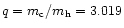 - mass-ratio of the components.
 |
 - gravity-darkening coefficients of the components.
 |
 - albedo coefficients of the components.
 |
|
- accepted metallicity of the components.
|
Note: n - number of observations,  (O-C)2 - final
sum of squares of residuals between observed (LCO) and synthetic (LCC) light
curves, (O-C)2 - final
sum of squares of residuals between observed (LCO) and synthetic (LCC) light
curves,  - standard deviation of the observation,
 - spots' temperature coefficients,
 , ,
 and
and
 - spots' angular dimensions,
longitudes and latitudes (in arc degrees),
- spots' angular dimensions,
longitudes and latitudes (in arc degrees),
 - limb-darkening
coefficients of the components,
- limb-darkening
coefficients of the components,
 - dimensionless surface
potentials of the common photosphere,
- dimensionless surface
potentials of the common photosphere,
 , ,
 -
the potentials of the inner and outer contact surfaces respectively,
-
the potentials of the inner and outer contact surfaces respectively,
![$f{\rm _{over}[\%]=100\cdot(\Omega_{1,2}-\Omega_{in})/(\Omega_{out}-
\Omega_{in})}$](/articles/aa/full/2001/09/aa9840/img73.gif) - degree of overcontact,
- degree of overcontact,
 - polar radii of the
components in units of the distance between the component centres,
- polar radii of the
components in units of the distance between the component centres,
 - luminosity of the hotter star (including spots on the
cooler one),
- luminosity of the hotter star (including spots on the
cooler one),
![$a_{\rm orb} [R_{\odot}]$](/articles/aa/full/2001/09/aa9840/img76.gif) - orbital semi-major axis in units of the solar
radius,
- orbital semi-major axis in units of the solar
radius,
![${\cal M}_{\rm h,c} [M_{\odot}]$](/articles/aa/full/2001/09/aa9840/img77.gif) - masses of components in
solar units,
- masses of components in
solar units,
![${\cal R}_{1,2} [R_{\odot}]$](/articles/aa/full/2001/09/aa9840/img78.gif) - mean radii of stars in solar
units,
- mean radii of stars in solar
units,
 - logarithm (base 10) of the mean surface
acceleration (effective gravity) for components and
- logarithm (base 10) of the mean surface
acceleration (effective gravity) for components and
 - absolute bolometric magnitudes of stars.
 |
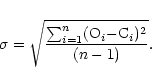
The solution for each individual light curve is presented in Fig. 1,
where the optimum fit of the observed light curves (LCO) to the
synthetic ones (LCC) is shown. The reference light level of Binnendijk's
1958 light curve at orbital phase 0.25, for the unspotted
configuration of the system is denoted by a dashed line. The rest of
the light curves are scaled to this light level. The O-C residuals
between the observed (LCO) and optimum synthetic (LCC) light curves are
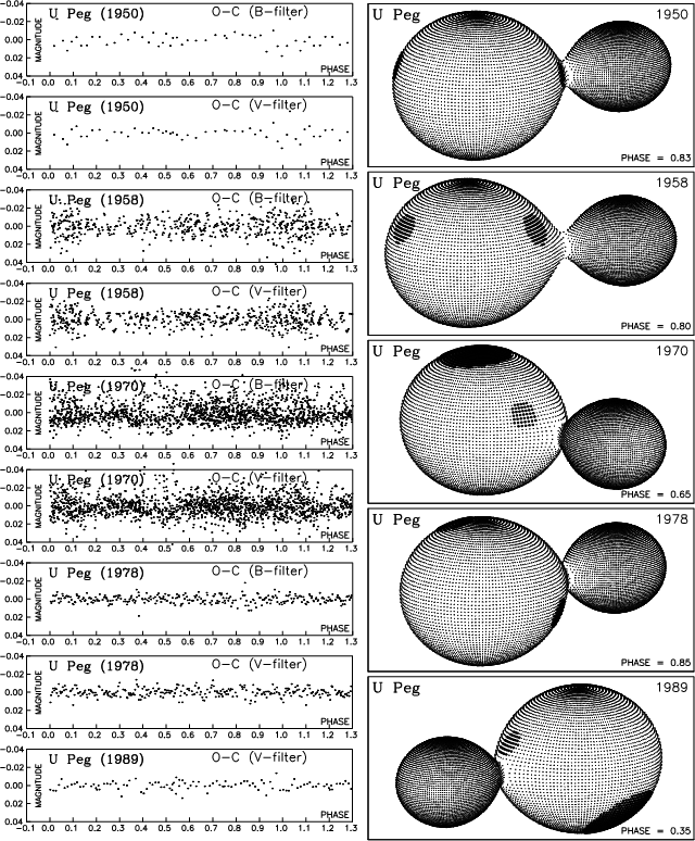
given on the left-hand sides of Fig. 2. The right-hand
side on these panels shows the view of Roche models of U Peg
obtained with the parameters estimated by analysing the corresponding light
curves. Using such plots, one sees how a CB system would look
at a certain orbital phase, chosen so that the spots are visible.
It is evident from Table 1 and from Figs. 1 and
2 (left) that the Roche model with spot areas on the cooler
component gives a satisfying fit of the analysed light curves.
In the case of two spotted areas on the cooler component, the Roche model
with the system's basic parameters that are constant for the whole set
of the analysed
light curves satisfyingly fits the observations. This indicates that the
complex nature of the light-curve variations during the examined period can
be explained by the evolution and motion of spotted areas across the
stellar surfaces.
The solutions presented here show that U Peg is in an overcontact
configuration
![$(f{\rm _{over}[\%] \sim 14.9\%)}$](/articles/aa/full/2001/09/aa9840/img81.gif) ,
with a
small temperature difference between the components
(
,
with a
small temperature difference between the components
(
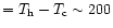 K) proving a good thermal contact between the
components. The mass-ratio estimated to
suggests a
significant energy transfer between the components through the connecting
neck of the common envelope.
The size of a spot area can be used as an indicator of the system's
activity. The analysis of the symmetric light curves from 1950 shows
only the presence of small spotted areas (located relatively close to the
stellar equator) which can produce a very small light-curve asymmetry.
It appears that the system is very probably in the minimum of the
spot activity during that period.
Later, the activity of the system increases, and the analysis of the light
curves from 1958 gives large spots on the same stellar hemispheres which cover
a significant part of the stellar surfaces. So, their presence leads to a
conspicuous asymmetry in the light curves. The spot locations from 1970
produce a light-curve asymmetry and a change in the light level at the maxima.
The larger spot is located at high latitude in the polar region, and the small
one is near the stellar equator. It seems that the system's activity decreases
after that year. The spot locations from 1978 practically do not affect the
symmetric shape of the light curves, but they change the light level at the maxima.
The observations made during November 1989 at the Observatorio Astronómico
Nacional at San Pedro Mártir with 84-cm reflecting telescope in Johnson's V
filter show large activity in the system again. It is possible that large spot
areas at high
latitudes (near stellar polar regions) correspond to an enhanced activity
of the system.
K) proving a good thermal contact between the
components. The mass-ratio estimated to
suggests a
significant energy transfer between the components through the connecting
neck of the common envelope.
The size of a spot area can be used as an indicator of the system's
activity. The analysis of the symmetric light curves from 1950 shows
only the presence of small spotted areas (located relatively close to the
stellar equator) which can produce a very small light-curve asymmetry.
It appears that the system is very probably in the minimum of the
spot activity during that period.
Later, the activity of the system increases, and the analysis of the light
curves from 1958 gives large spots on the same stellar hemispheres which cover
a significant part of the stellar surfaces. So, their presence leads to a
conspicuous asymmetry in the light curves. The spot locations from 1970
produce a light-curve asymmetry and a change in the light level at the maxima.
The larger spot is located at high latitude in the polar region, and the small
one is near the stellar equator. It seems that the system's activity decreases
after that year. The spot locations from 1978 practically do not affect the
symmetric shape of the light curves, but they change the light level at the maxima.
The observations made during November 1989 at the Observatorio Astronómico
Nacional at San Pedro Mártir with 84-cm reflecting telescope in Johnson's V
filter show large activity in the system again. It is possible that large spot
areas at high
latitudes (near stellar polar regions) correspond to an enhanced activity
of the system.
![\begin{figure}
\par\includegraphics[width=17.8cm,clip]{9840f1.eps}\end{figure}](/articles/aa/full/2001/09/aa9840/Timg84.gif) |
Figure 1:
Observed (LCO) and final synthetic (LCC) light curve of U Peg.
The reference light level of Binnendijk's 1958 light curve, at orbital phase
0.25, for the unspotted configuration of the system is shown by the dashed line |
 |
Figure 2:
Left: Final O-C residuals obtained by solving the inverse problem
within the framework of the Roche model with spotted areas on the cooler
component; Right: The view of the Roche model for U Peg at the noted orbital
phase, obtained with parameters estimated by solving the inverse problem |
| Open with DEXTER |
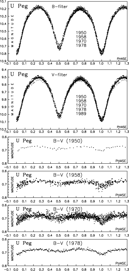
Finally, Fig. 3 presents observations of U Peg drawn together
for the B and V filters respectively, and the corresponding
colour-index B-V drawn for each epoch separately.
During the analysed period, the main variations in the light curves are in the
height of both maxima as well as in the depth of the light-curve minima. The
B-V colour-index for the whole set of the analysed light curves shows some
reddening around the light-curve minima. This effect may be attributed to the
temperature differences between the components, and partially to the
influence of spot active regions.
Both presentations of our results obtained in the analysis of U Peg
light curves between 1950 and 1989 (Table 1 and the
corresponding figures) show that the Roche model with spot
areas on the cooler component provides a satisfying fit of the observations.
During that period, the main variations in the light curves
can be explained by the change in the temperature contrast, and the position
and the size of spot areas on the cooler component. Having in mind that
we used the same basic system parameters for different curves, these
results indicate that the complex nature of the light-curve variations
may be attributed to variable starspot activity.
Moreover, several attempts were made to fit the observations by
assuming a spot model with spots on both components. In that
case we can obtain fits which are similar in quality, but for this we need
some variations of the system's basic parameters derived by analysing
the individual light curves around a mean value. We consider that case
as less reliable, such that we feel it to be possibly excluded.
The present analysis shows that the changes in the light curves can be
relatively well interpreted by the development and migration of spot
regions on the cooler component. The model can successfully simulate
the observed light curves which cover an interval of 39 years.
Our analysis shows that during the deeper (primary) minimum the cooler
(more massive and larger) component eclipses the hotter (less massive and
smaller) one. The solutions presented here show that U Peg is in the
over-contact configuration
,
with
a small temperature difference between the components (
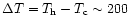 K) indicating a good thermal
contact between the components. The mass-ratio estimated to
suggests a significant energy transfer
between the components.
K) indicating a good thermal
contact between the components. The mass-ratio estimated to
suggests a significant energy transfer
between the components.
Having in mind the large changes in the shape of the light curves, future
photometric observations of this interesting system are of great interest.
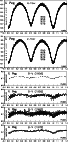 |
Figure 3:
Observations of U Peg drawn together for B and V filters
respectively, and corresponding B-V colour-index drawn for each year
separately |
| Open with DEXTER |
Acknowledgements
Three of us (G. D., S. E. & N. M.) have been partially supported by the
Ministry for Sciences and Technology of Serbia through the project
"Astrometrical, Astrodynamical and
Astrophysical investigations''.
H. R.-L. & P. R. acknowledge some financial support from Athens University
and the National Observatory of Athens.
- Adams, W. S., Joe, A. H., & Sanford, R. F. 1924, PASP, 36, 139
In the text
- Adams, W. S., Joe, A. H., Humason, M. L., & Brayton, A. M. 1924, ApJ, 81, 187
In the text
NASA ADS
- Binnendijk, L. 1960, AJ, 65, 88
In the text
NASA ADS
- Carbon, D., & Gingerich, O. 1969, in Theory and Observation of Normal
Stellar Atmospheres, ed. O. Gingerich (MIT Press, Cambridge), 377
In the text
- Chandler, S. C. 1895, AJ, 15, 181
In the text
NASA ADS
- Díaz-Cordovés, J., Claret, A., & Giménez, A. 1995, A&AS, 110, 329
In the text
NASA ADS
- Djurasevic, G. 1992a, Ap&SS, 196, 241
In the text
NASA ADS
- Djurasevic, G. 1992b, Ap&SS, 197, 17
In the text
NASA ADS
- Djurasevic, G., Zakirov, M., Hojaev, A., &
Arzumanyants, G. 1998, A&AS, 131, 17
In the text
NASA ADS
- La Fara, R. 1952, ApJ, 115, 14
NASA ADS
- Lafta, S. J., & Grainger, J. F. 1986, Ap&SS, 121, 61
In the text
NASA ADS
- Lejeune, T., Cuisinier, F., & Buser, R. 1997, A&AS, 125, 229
In the text
NASA ADS
- Lejeune, T., Cuisinier, F., & Buser, R. 1998, A&AS, 130, 65
In the text
NASA ADS
- Lu, W. X. 1985, PASP, 97, 1086
In the text
NASA ADS
- Lucy, L. B. 1967, Zs. f. Ap., 65, 89
In the text
- Lucy, L. B., & Wilson, R. E. 1979, ApJ, 231, 502
In the text
NASA ADS
- Marquardt, D. W. 1963, J. Soc. Ind. Appl. Math., 11, No. 2, 431
In the text
- Maupomé, L., Rodríguez, E. Hobart, M. A., Peña, J. H., & Peniche, R. 1991, Rev. Mexicana Astron Astrof., 22, 235
In the text
NASA ADS
- Press, W. H., Teukolsky, S. A., Vetterling, W. T., & Flannery, B. P. 1992, Numerical Recipes in Fortran, The Art of Scientific Computing, Second Edition (Cambridge
University Press, New York), 120
In the text
- Rafert, J. B., & Twigg, L. W. 1980, MNRAS, 139, 78
In the text
- Rigterink, P. V. 1972, AJ, 77, 319
In the text
NASA ADS
- Rucinski, S. M. 1969, Acta Astr., 19, 245
In the text
- Rucinski, S. M., & Duerbeck, H. W. 1997, PASP, 109,
1340
In the text
NASA ADS
- Russo, G., Sollazzo, C, Maceroni, C., & Milano, L. 1982,
A&AS, 47, 211
In the text
NASA ADS
- Struve, O., Horak, H. G., Canavaggia, R., Kourganoff, V., & Colachevich, A. 1950, ApJ, 111, 658
In the text
- Vaz, L. P. R., Anderson, J., & Rabello Soares, M. C. A. 1995, A&A, 301, 69
In the text
- Wilson, R. E., & Devinney, E. J. 1971, ApJ, 166, 605
In the text
NASA ADS
- Zhai, D. S., Leung, K. C., & Zhang, R. X. 1984, A&AS, 57, 487
In the text
NASA ADS
- Zhai, D. S., Lu, W. X., & Zhang, X. Y. 1988, Ap&SS, 146, 1
In the text
NASA ADS
Copyright ESO 2001

![\begin{figure}
\par\includegraphics[width=17.8cm,clip]{9840f1.eps}\end{figure}](/articles/aa/full/2001/09/aa9840/img84.gif)