A&A 367, 199-210 (2001)
DOI: 10.1051/0004-6361:20000413
A. Skopal1![]() -
M. Teodorani2 - L. Errico2 - A. A. Vittone2 - Y. Ikeda3 - S. Tamura3
-
M. Teodorani2 - L. Errico2 - A. A. Vittone2 - Y. Ikeda3 - S. Tamura3
1 - Astronomical Institute, Slovak Academy of Sciences, 05960 Tatranská Lomnica, Slovakia
2 - Osservatorio Astronomico di Capodimonte, via Moiariello 16, 80131 Napoli, Italy
3 - Astronomical Institute, Tohoku University, Sendai 980-8578, Japan
Received 27 July 2000 / Accepted 7 November 2000
Abstract
We analysed photometric and spectroscopic optical observations of
the eclipsing symbiotic binary AXPersei. For the first time, we
present and discuss its historical, 1887-1999, photographic/B-band and visual light curve (LC).
The red giant in AXPer losses mass via the wind at a rate of
![]() .
The terminal velocity of the wind is
.
The terminal velocity of the wind is
![]() .
We estimated an effective radius of the H II nebula during the post-outburst stage (to JD2450000) to be of
.
We estimated an effective radius of the H II nebula during the post-outburst stage (to JD2450000) to be of
![]() and its average electron concentration
and its average electron concentration
![]() for the electron temperature
for the electron temperature
![]() = 1-1.5 104K. The [O III] nebula in AXPer is rather dense, having the electron concentration
= 1-1.5 104K. The [O III] nebula in AXPer is rather dense, having the electron concentration ![]() ([O III])
([O III])
![]() for
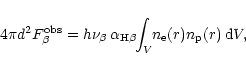
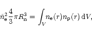
for ![]() = 1-1.5 104K. Spectroscopic observations made in the middle of the 1992.8 and 1994.7 eclipses showed that a significant part of flux emitted in the H I, He II and nebular [O III] lines originates in the vicinity of the hot component. Transition of AXPer to its nebular phase occurred at/around JD2450000. A small
= 1-1.5 104K. Spectroscopic observations made in the middle of the 1992.8 and 1994.7 eclipses showed that a significant part of flux emitted in the H I, He II and nebular [O III] lines originates in the vicinity of the hot component. Transition of AXPer to its nebular phase occurred at/around JD2450000. A small ![]() 0.6mag brightening at that time and consequently very broad wave-like variation in the LC developed. This event was caused by dilution of a shell around the hot star, during which about of
1.5 1050 particles (
0.6mag brightening at that time and consequently very broad wave-like variation in the LC developed. This event was caused by dilution of a shell around the hot star, during which about of
1.5 1050 particles (![]()
![]() )
were injected into the ionized region.
)
were injected into the ionized region.
Key words: stars: binaries: symbiotics - stars: circumstellar matter - stars: mass-loss
At present, AXPer is known as an eclipsing symbiotic binary with
an orbital period of 680 days (Skopal 1991).
The cool component of the binary is a normal giant of the spectral
type M4.5 (Mürset & Schmid 1999). Its effective temperature,
![]() K,
was recently determined by Skopal (2000) by comparing the observed
broad-band optical/IR photometry to synthetic spectra for cool giants.
Mikolajewska & Kenyon (1992) determined the mass ratio,
K,
was recently determined by Skopal (2000) by comparing the observed
broad-band optical/IR photometry to synthetic spectra for cool giants.
Mikolajewska & Kenyon (1992) determined the mass ratio,
![]() = 2.4,
by solving the spectroscopic orbit of AXPer for both components.
Mürset et al. (1991) derived the temperature of the hot
component,
= 2.4,
by solving the spectroscopic orbit of AXPer for both components.
Mürset et al. (1991) derived the temperature of the hot
component,
![]()
![]() 105 K,
and its luminosity,
105 K,
and its luminosity,
![]() ,
by using their modified Zanstra method for the recombination line
He II1640Å.
,
by using their modified Zanstra method for the recombination line
He II1640Å.
Other fundamental parameters for AXPer are known within the
uncertainty given by limiting values of the orbital inclination:
(i) If the giant fills its tidal lobe (
![]() ),
the orbital inclination is
),
the orbital inclination is
![]() ,
which implies
the stellar masses
,
which implies
the stellar masses
![]() and
and
![]() (Mikolajewska & Kenyon 1992).
(ii) In the case of
(Mikolajewska & Kenyon 1992).
(ii) In the case of
![]() ,
the giant's radius
,
the giant's radius
![]() (Skopal 1994)
and the distance
(Skopal 1994)
and the distance
![]() pc (Skopal 2000).
Quantities of the latter case agree well with those obtained from
empirically determined dependencies of effective temperature upon
spectral type (cf. van Belle et al. 1999; Skopal 2000).
Also, Mürset & Schmid (1999) suggest that AXPer is
a well detached binary.
pc (Skopal 2000).
Quantities of the latter case agree well with those obtained from
empirically determined dependencies of effective temperature upon
spectral type (cf. van Belle et al. 1999; Skopal 2000).
Also, Mürset & Schmid (1999) suggest that AXPer is
a well detached binary.
![\begin{figure}
\par\includegraphics[width=12cm,clip]{ms10145f1.eps} \end{figure}](/articles/aa/full/2001/07/aa10145/img30.gif) |
Figure 1: The historical LC of AXPer. It is compiled from photographic measurements published by Lindsay (1932), Payne-Gaposchkin (1946), Wenzel (1956) and Mjalkovskij (1977), visual magnitude estimates gathered by members of the Association Française des Observateurs d'Étoiles Variables, which are available on CDS (smoothed within 20-day bins), and from photoelectric B magnitudes from Table 2 |
The quiescent phase of AXPer is sometimes interrupted by 2-3 mag optical eruptions. The nature of the outburst stage is not well understood. Different models explaining the behaviour during outbursts have been developed. Mikolajewska & Kenyon (1992) suggested that the system contains a red giant that fills its tidal lobe and transfers material into an accretion disk surrounding a low mass main sequence star. They ascribed the phase-dependent modulation of the light at the 2-mag level to superhumps resulting from a resonance interaction between the disk and the mass losing giant. Skopal (1994) suggested a model in which the material ejected during the outburst impacts the giant and creates a collisionally excited emission region on its hemisphere facing the hot star. The wave-like orbital modulation of the optical continuum then results from its different visibility at different orbital phases.
This contribution is in major part devoted to studying a transition period of AXPer from its recent (1988-90) activity to the present quiescent (nebular) phase. In Sect. 2 we give a description of our observations with a special emphasis on the historical, 1887-1999, LC. In Sect. 3 we analyze our observations, trying to determine some parameters of the system, and to identify physical processes which are responsible for the observed properties.
Our spectroscopic observations were taken during the recent 1989 outburst and the following quiescent phase.
High-dispersion spectroscopy was secured at the Asiago Astrophysical
Observatory with the REOSC Echelle Spectrograph (RES) equipped with
a CCD detector mounted at the Cassegrain focus of the 1.82-m telescope
at Mt. Ekar. The telescope is operated by the Astronomical Observatory of
Padova.
In 1998 the RES spectrograph was equipped with a Thompson THX31156
UV-coated CCD detector,
![]() pixels of
pixels of ![]() m size. Dispersions
of 3.1, 3.2, 4.0 and 4.5 Å mm-1 were obtained in the ranges
4330-4460, 4800-4940, 5800-5990 and 6480-6670 Å, respectively.
Exposures of 60 min were used.
The RES echelle orders were straightened through the software developed
at the Astronomical Observatory of Capodimonte in Napoli. Thereafter,
the spectroscopic data were processed by using the ESO MIDAS software
package in the following steps:
(i) Flat field and bias subtraction,
(ii) sky-background subtraction,
(iii) calibration in wavelength using a thorium lamp for comparison lines
and
(iv) correction for heliocentric velocity.
m size. Dispersions
of 3.1, 3.2, 4.0 and 4.5 Å mm-1 were obtained in the ranges
4330-4460, 4800-4940, 5800-5990 and 6480-6670 Å, respectively.
Exposures of 60 min were used.
The RES echelle orders were straightened through the software developed
at the Astronomical Observatory of Capodimonte in Napoli. Thereafter,
the spectroscopic data were processed by using the ESO MIDAS software
package in the following steps:
(i) Flat field and bias subtraction,
(ii) sky-background subtraction,
(iii) calibration in wavelength using a thorium lamp for comparison lines
and
(iv) correction for heliocentric velocity.
Additional high-dispersion spectroscopy was secured
at the Okayama Astrophysical Observatory (OAO) with the 74-inch Coudé
spectrograph using an intensified Reticon. The spectra were centered
on the regions of H![]() ,
[O III]5007Å and
He II4686Å lines with a dispersion of 5.24, 5.49 and
5.50Åmm-1, respectively. The data were treated by using
the IRAF software package. A standard procedure of (i) dark subtraction,
(ii) flattening, (iii) wavelength calibration with the Th-Ne lamp,
and (iv) correction for heliocentric velocity, was applied.
,
[O III]5007Å and
He II4686Å lines with a dispersion of 5.24, 5.49 and
5.50Åmm-1, respectively. The data were treated by using
the IRAF software package. A standard procedure of (i) dark subtraction,
(ii) flattening, (iii) wavelength calibration with the Th-Ne lamp,
and (iv) correction for heliocentric velocity, was applied.
A medium-dispersion spectrogram (17Åmm-1) was obtained with a grating spectrograph mounted in the Coudé focus of the 2-m telescope at the Ondrejov Observatory. The spectrogram was exposed on a Kodak IIa-O plate, covering the optical region from 3600Å to 4900Å, and was analyzed by the 5-channel microphotometer at the Ondrejov Observatory using the SPEFO software (Horn 1992).
The continuum of all spectra was scaled to fluxes determined by (near-)simultaneous photometric measurements, which we dereddened with EB-V = 0.27. The conversion between the magnitude system and corresponding fluxes was made according to Henden & Kaitchuck (1982). The log of our spectroscopic observations is given in Table 1.
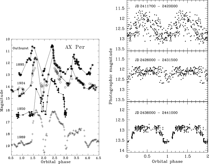 |
Figure 2:
Left: the main outbursts of AXPer. The phase dependent
ingress/egress modulation of the light at the 2-mag level represents
a dominant feature of each outburst. Sources of the data:
( |
| Date | Orbital | Exp. | Wavelength | Obs.b |
| phasea | [s] | [Å] | ||
| 1989 Nov. 30 | 0.46 | 10800 | 3600-4900 | O |
| 1992 Oct. 13 | 0.00 | 3600 | 4330-5400 | A |
| 1993 Nov. 1 | 0.56 | 270 | 6490-6600 | OAO |
| 1993 Nov. 3 | 0.56 | 540 | 4630-4750 | OAO |
| 1993 Nov. 5 | 0.57 | 600 | 4950-5060 | OAO |
| 1994 Aug. 19 | 0.99 | 900 | 4950-5060 | OAO |
| 1994 Aug. 20 | 0.99 | 900 | 6490-6600 | OAO |
| 1994 Aug. 21 | 0.99 | 1200 | 4630-4750 | OAO |
| 1994 Dec. 12 | 0.15 | 720 | 4950-5060 | OAO |
| 1998 Jan. 9 | 0.81 | 3600 | 4330-6670 | A |
| 1998 Sep. 5 | 0.16 | 3600 | 4330-6670 | A |
Photometric observations used in this paper consist of photographic
measurements summarized from the literature (see Fig. 1), as well
as standard broad-band UBVR photoelectric photometry and visual
magnitude estimates available from the CDS. Our photoelectric
measurements were performed using a single-channel photon-counting
device mounted at the Cassegrain foci
of 0.6-m reflectors at the Skalnaté Pleso and Stará Lesná
Observatories. The star BD+54331 (HD9839, SAO22444, V=7.43,
B-V = 1.02,
U-B = 0.63) and the neighbouring star
(
![]() )
were used as comparison and check stars, respectively. We measured
the check star with respect to the comparison and found its brightness
as V = 9.48,
B-V = 1.37,
U-B = 1.20.
Observations are listed in Table 2.
Each value represents the average of the observations taken during
a single night. The uncertainty of these night-means is of
a few
)
were used as comparison and check stars, respectively. We measured
the check star with respect to the comparison and found its brightness
as V = 9.48,
B-V = 1.37,
U-B = 1.20.
Observations are listed in Table 2.
Each value represents the average of the observations taken during
a single night. The uncertainty of these night-means is of
a few
![]() mag in the V and B bands, and up to 0.02mag
in the U band.
mag in the V and B bands, and up to 0.02mag
in the U band.
The historical (1887-1999) LC of AXPer is depicted in Fig. 1. It is characterized by long-lasting periods of quiescence (in contrast to BFCyg: see Fig. 1 of Skopal et al. 1997), with superposition of a few bright stages lasting about 1.5 orbital cycles.
The left panel of Fig. 2 shows in detail four main phases of activity
observed from the end of the last century (1895, 1924, 1950 and 1989).
The rise to a maximum of brightness begins around orbital phase
![]() 0.5 and follows the same type of variation during
each outburst. It exhibits two dominant
features: first, deep minima caused by eclipses of the hot star by
the red giant (orbital phase
0.5 and follows the same type of variation during
each outburst. It exhibits two dominant
features: first, deep minima caused by eclipses of the hot star by
the red giant (orbital phase
![]() ), and second, a wave-like
modulation at the 2-mag level. The latter varies as a function of
orbital phase with a maximum of light around
), and second, a wave-like
modulation at the 2-mag level. The latter varies as a function of
orbital phase with a maximum of light around
![]() .
The modulation disappears after about 1.5 orbital cycles. It is
obvious that such behaviour reflects a geometrical effect.
Skopal (1994)
explained this modulation by varying visibility of a collisionally
excited emission region located on the red giant hemisphere
facing the hot star. The emission region on the giant star results
from the impact of material ejected by the hot star during outbursts.
.
The modulation disappears after about 1.5 orbital cycles. It is
obvious that such behaviour reflects a geometrical effect.
Skopal (1994)
explained this modulation by varying visibility of a collisionally
excited emission region located on the red giant hemisphere
facing the hot star. The emission region on the giant star results
from the impact of material ejected by the hot star during outbursts.
During the quiescent phase, the star's brightness varies periodically
between about 12 and 13.5 mag. The LC displays typical wave-like
modulation, which is connected to orbital motion.
We folded the data from quiescent phases into a phase diagram
according to the ephemeris for the minima
| (1) |
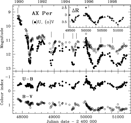 |
Figure 3:
The UBV and |
![\begin{figure}
\includegraphics[width=7.5cm,clip]{ms10145f4.eps}\end{figure}](/articles/aa/full/2001/07/aa10145/img40.gif) |
Figure 4: Variation in the profile of the minima during different epochs. Top: phase diagram of Mjalkovski's (1977) data from the 1958-1972 period (open circles mirror the data observed prior to phase 1.0). Middle: minima observed during the transition period from the recent outburst to the present quiescence. Bottom: the broad wave-like minima which developed after 1995.8 |
Our photoelectric UBVR measurements cover a transition period of
AXPer from its recent (1989) active phase to the present quiescence,
until 1999.3 (Fig. 3). The most interesting variation can be seen
in the evolution of the minima profile. Prior to JD2450000 (1995.8),
they were narrow with broader ingress/egress wings, and were more pronounced
at the 1992.8 and 1994.7 minima (middle panel of Fig. 4).
The deep, narrow
core of these eclipses implies the presence of a component of radiation
located close to the hot star. This is probably due to the fact that
a shell, which was created in maximum, still persisted around the hot
star and redistributed a fraction of its radiation into the optical.
On the other hand, the broader wings accompanying the central core of
the eclipse profile indicate the simultaneous presence of a nebula
extended around the hot component (see Sect. 3.2 for more detail).
In addition, we can see
that the depth of minima in V became shallower after the outburst
stage. The B-V colour index increased from ![]() 0.6 in 1990 to
0.6 in 1990 to
![]() 1.4mag in 1999. A larger change by
1.4mag in 1999. A larger change by ![]() 0.3mag occured
after 1995.8, when the nebular continuum dominated the optical
spectrum (see Sect. 3.5).
0.3mag occured
after 1995.8, when the nebular continuum dominated the optical
spectrum (see Sect. 3.5).
A drastic change in the LC profile occured after a brightening
of about 0.6mag, observed at JD2450000 (October 1995).
The narrow minima
observed prior to this time developed abruptly in very broad waves
(bottom panel of Fig. 4). The minima were still located around the
position of the inferior conjunction of the giant star, but their
centres are shifted by ![]() 10 days from the position predicted
by the ephemeris (1). The amplitude is similarly wavelength dependent,
as observed for other symbiotics with such
type of variation (
10 days from the position predicted
by the ephemeris (1). The amplitude is similarly wavelength dependent,
as observed for other symbiotics with such
type of variation (
![]() ).
During this period, the maximum level of the star's brightness
decreased by about 0.5, 0.2 and 0.1mag in the UB,
V and R
bands, respectively. Simultaneously, the colour indices, mainly
the U-B index, display a sinusoidal variation along the orbit.
).
During this period, the maximum level of the star's brightness
decreased by about 0.5, 0.2 and 0.1mag in the UB,
V and R
bands, respectively. Simultaneously, the colour indices, mainly
the U-B index, display a sinusoidal variation along the orbit.
| Element | Wavelength | |||
| [Å] | Nov. 1993 | Aug. 1994 | Dec. 1994 | |
| N III | 4634.160 | 2.5/4.4/3.0 | - | - |
| N III | 4640.640 | 8.8/8.4/3.0 | - | - |
| He II | 4685.682 | 60.2/34.5/3.0 | 24.0/17.2/1.6 | - |
| [O III] | 4958.910 | 37.1/29.4/3.0 | 18.0/18.8/1.5 | 31.5/28.9/3.2 |
| [O III] | 5006.840 | 103.6/77.4/3.0 | 59.4/47.7/1.7 | 98.2/76.0/3.2 |
| He I | 5015.675 | 4.9/5.4/3.0 | 1.2/1.8/1.5 | 3.5/4.9/ 3.2 |
| H I | 6562.817 | 701.8/254.1/4.4 | 144.1/72.6/4.0 | - |
The spectrum of AXPer, which developed during the last, 1988-90, active phase, has already been described by several authors (Skopal & Komárek 1990; Mikolajewska & Kenyon 1992; Ivison et al. 1993). Generally, the spectrum resembles that of a low ionization shell spectrum, characterized by strong lines of H I with a complex double-peaked profile and numerous fainter lines of mainly Fe II and Ti II (Fig. 5). The continuum around the Balmer jump was flat.
The spectrum from the post-outburst phase (our spectrograms from 13/10/92, 1-5/11/93, 19-21/8/94, 9/1/98 and 5/9/98) resembled that of a typical symbiotic spectrum of a quiescent phase. The line spectrum was characterized by strong emissions of H I, He I, He II, [O III], [Ca V], [Fe VI], [Fe VII] and N III. The lines of [O III], He I and He II exhibited single narrow profiles. Numerous Fe I absorptions and TiO bands were also present.
After JD2450000, a significant change occured in the line spectrum. Prior to this time, all emissions, but mainly the [O III] lines, dominated the spectrum. After October 1995 the line fluxes decreased (Fig. 5, Table 3) and the profiles of [Fe VI], [Fe VII] and [Ca V] lines consisted of two components (Figs. 5, 9). This change was probably caused by the larger opacity of the more extended nebula, which developed after 1995.8 (see Sect. 3.5). In this case, the radial velocity field of the line emission regions was more complex, which could result in two (or possibly more) component profiles of some species.
The H I lines displayed single profiles, in contrast to the active phase. However, they were affected by an absorption, mainly on the violet side (Figs. 5, 9). Such behaviour was recently observed also for BFCyg (Skopal et al. 1997). Analysis of the H I lines is described in Sect. 3.4.
Basic characteristics of the line spectrum of our spectra are shown
in Figs. 5 and 6. Tables 3 and 4 summarize the observed
spectrophotometric
parameters of individual lines. The emission line fluxes were measured
using our own code. The level of the local continuum was estimated
by eye. A high level of the signal-to-noise ratio of our spectra
allowed us to measure the line parameters with an uncertainty of a few
percent. Only in the case of the spectra observed at OAO during
the 1994 eclipse was the continuum more poorly defined. As a result,
the uncertainty in line fluxes is about 15-20% for He II and
[O III], and less then 10% for H![]() .
.
The phased photographic LC, which was measured by Mjalkovskij
(1977)
during the quiescent phase between 1958 and 1972, displays a very
broad, but nearly rectangular, minimum. The bottom part
is nearly flat and lasted from the orbital phase
![]() to
to ![]() 1.1 (Fig. 4 top).
This suggests that the eclipsed region occupied a large volume
during that period, and thus could not be of stellar nature.
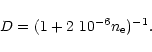
It is well known that during quiescent phases, the nebular continuum
dominates the optical region. The hot
star (
1.1 (Fig. 4 top).
This suggests that the eclipsed region occupied a large volume
during that period, and thus could not be of stellar nature.
It is well known that during quiescent phases, the nebular continuum
dominates the optical region. The hot
star (
![]() K) ionizes a portion of the cool
star wind and gives rise to the recombination continuum. The extent
of the ionized zone can be obtained from a parametric equation
K) ionizes a portion of the cool
star wind and gives rise to the recombination continuum. The extent
of the ionized zone can be obtained from a parametric equation
![\begin{figure}
\par\includegraphics[width=7cm,clip]{ms10145f7.eps} \end{figure}](/articles/aa/full/2001/07/aa10145/img51.gif) |
Figure 7:
The H I/H II boundary calculated for
three models of the stellar wind distinguished by the parameter
|
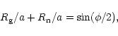
The eclipse profile puts limits to the extension of the ionized
region, which is subject to eclipse. According to Eq. (2) it is
a function of the parameter X. The ingress to the minimum started
at
![]() and the egress ended at
and the egress ended at
![]() .
It means that the lines of sight at these phases represent
the limits for maximum opening of the H II zone in AXPer
during that time (Fig. 7). Therefore we calculated the
H I/H II boundary in order to match these lines.
In this way, we obtained the parameter X = 0.35, 0.65 and 1.0,
corresponding to
.
It means that the lines of sight at these phases represent
the limits for maximum opening of the H II zone in AXPer
during that time (Fig. 7). Therefore we calculated the
H I/H II boundary in order to match these lines.
In this way, we obtained the parameter X = 0.35, 0.65 and 1.0,
corresponding to ![]() ,
1.25 and 2.5, respectively, in
the stellar wind model (5).
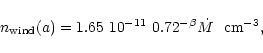
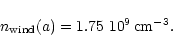
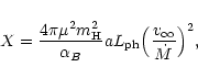
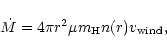
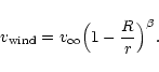
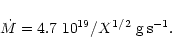
Independently, relation (3) enables us to determine the mass loss
rate,
,
1.25 and 2.5, respectively, in
the stellar wind model (5).
Independently, relation (3) enables us to determine the mass loss
rate, ![]() ,
as a function of X for the known parameters
of the binary. For AXPer, the hot star bolometric luminosity of
,
as a function of X for the known parameters
of the binary. For AXPer, the hot star bolometric luminosity of
![]() (
(
![]() for
for
![]() pc; Skopal 2000)
and the temperature
pc; Skopal 2000)
and the temperature
![]() K (Mürset et al. 1991)
give the rate of ionizing photons
K (Mürset et al. 1991)
give the rate of ionizing photons
![]() .
Then, the quantities
.
Then, the quantities
![]() (resulting from
(resulting from
![]() ,
,
![]() and
and
![]() days, Sect. 1),
days, Sect. 1),
![]() (Skopal 1994),
(Skopal 1994),
![]() (Sect. 3.4 below),
(Sect. 3.4 below),
![]() and
and
![]() transform Eq. (3) into
transform Eq. (3) into
| X | ||
|
|
||
| 0.35 | 0 | |
|
|
0.65 | 1.25 |
|
|
1.0 | 2.5 |
During the post outburst stage, from about 1990 to 1995, small
ingress/egress wings developed in the 1992.8 and 1994.7 minima
profiles (Fig. 4 mid).
This feature obviously reflects the presence of a nebula extended
around the hot component, caused by an increase in its temperature.
This view is supported by the presence of very strong nebular
and He II lines (Figs. 5, 6, Tables 3, 4), which
were absent or very faint during the maximum. The nebula was relatively
stable in size as well as optical properties until October 1995
(![]() JD2450000). This is indicated by fluxes of the
[O III] lines, which did not change during this period (within
10-15% uncertainty of their determination), but in both eclipses
were lower by about 50% of their out-of-eclipse values. As we did
not observe any other significant brightness variation along the
orbital cycle, we can assume that the nebula was optically thin
during that period. Under such conditions, a maximum of the observed flux,
JD2450000). This is indicated by fluxes of the
[O III] lines, which did not change during this period (within
10-15% uncertainty of their determination), but in both eclipses
were lower by about 50% of their out-of-eclipse values. As we did
not observe any other significant brightness variation along the
orbital cycle, we can assume that the nebula was optically thin
during that period. Under such conditions, a maximum of the observed flux,
![]() (in
(in
![]() ), in the line
H
), in the line
H![]() can be obtained from the equation
can be obtained from the equation
 |
(8) |
 |
(10) |
 |
(11) |
To check the reality of the
![]() density,
we compared its value to the particle density given by the mass
loss rate of the giant, derived in Sect. 3.1. According to
Eqs. (4) and (5) and the parameters for AXPer (the end of Sect. 3.1),
we can write the particle density at the distance a from the giant's
center as
density,
we compared its value to the particle density given by the mass
loss rate of the giant, derived in Sect. 3.1. According to
Eqs. (4) and (5) and the parameters for AXPer (the end of Sect. 3.1),
we can write the particle density at the distance a from the giant's
center as
 |
(12) |
 |
(13) |
![\begin{figure}
\par\includegraphics[width=8.5cm,clip]{ms10145f8.eps} \end{figure}](/articles/aa/full/2001/07/aa10145/img118.gif) |
Figure 8:
Dependence of the electron concentration |
To estimate these parameters in the nebula of AXPer, we
employed the well-known method based on the observed fluxes
of [O III]4363 and the nebular
N1, N2 ([O III]5007
and [O III]4959) lines. A theoretical dependence of
![]() and
and ![]() on the ratio, R, of these lines
can be written as (e.g. Gurzadyan 1997)
on the ratio, R, of these lines
can be written as (e.g. Gurzadyan 1997)
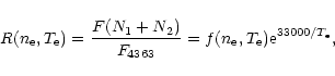 |
(14) |
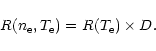
Electron densities, ![]() ([O III]), are limited by real
temperatures (
([O III]), are limited by real
temperatures (
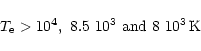
![]() K), which put lower limit of
K), which put lower limit of
![]() for the measured values of R (Fig. 8). The upper limit is then
given by densities in the H II zone around
the hot star, being of
for the measured values of R (Fig. 8). The upper limit is then
given by densities in the H II zone around
the hot star, being of ![]()
![]() (Sect. 3.2).
This limit can be determined more precisely if we consider
a deactivation of nebular transitions. This process of line
weakening takes place when the electron concentration is higher
than a critical value for the nebular line under consideration.
For the nebular N1 and N2 lines the deactivation factor is
(Sect. 3.2).
This limit can be determined more precisely if we consider
a deactivation of nebular transitions. This process of line
weakening takes place when the electron concentration is higher
than a critical value for the nebular line under consideration.
For the nebular N1 and N2 lines the deactivation factor is
 |
(15) |
 |
(16) |
![\begin{displaymath}n_{\rm e}([O{\sc iii}]) \approx 3~10^{7}\,\rm cm^{-3}.
\end{displaymath}](/articles/aa/full/2001/07/aa10145/img132.gif)
![\begin{figure}
\par\includegraphics[width=16.8cm,clip]{ms10145f9.eps} \end{figure}](/articles/aa/full/2001/07/aa10145/img133.gif) |
Figure 9: Examples of fitting the observed profiles (thin full line) by Gaussian functions. Emission components are drawn by broken lines, and the resulting fit by thick full lines |
We corrected the observed fluxes of H![]() ,
H
,
H![]() and H
and H![]() for an absorption originating from the cool
component wind. Therefore
we de-convolved the observed profile into an emission component,
emerging from the H II zone, and an absorption component, having
its origin in the H I zone (Fig. 9). In accordance with this view,
the radial velocity of the H
for an absorption originating from the cool
component wind. Therefore
we de-convolved the observed profile into an emission component,
emerging from the H II zone, and an absorption component, having
its origin in the H I zone (Fig. 9). In accordance with this view,
the radial velocity of the H![]() absorption component is the sum
of the space velocity of the system, the cool star
orbital motion, and the velocity of the neutral gas
with respect to the giant, which is assumed to be close to the
terminal velocity of the giant's wind,
absorption component is the sum
of the space velocity of the system, the cool star
orbital motion, and the velocity of the neutral gas
with respect to the giant, which is assumed to be close to the
terminal velocity of the giant's wind,
![]() .
The values of -150, -160, -150 and -136kms-1 obtained from fitting H
.
The values of -150, -160, -150 and -136kms-1 obtained from fitting H![]() profiles on 1/11/93, 20/8/94, 9/1/98
and 5/9/98 spectra, respectively, suggest the terminal velocity of the giant's wind to be
profiles on 1/11/93, 20/8/94, 9/1/98
and 5/9/98 spectra, respectively, suggest the terminal velocity of the giant's wind to be
The right panel of Fig. 6 shows a drastic change in the H![]() profile due to the eclipse of the hot star by its giant companion.
The observed flux decreased by factor of
profile due to the eclipse of the hot star by its giant companion.
The observed flux decreased by factor of ![]() 5, and the broad wings,
extending to
5, and the broad wings,
extending to ![]() 550kms-1 on 1/11/93, shrank to about
550kms-1 on 1/11/93, shrank to about
![]() 200kms-1 in the eclipse on 20/8/94. This means that
the ionized region in the vicinity of the hot star, within the radius
of the giant stellar disk, contributes significantly to the emission in
H
200kms-1 in the eclipse on 20/8/94. This means that
the ionized region in the vicinity of the hot star, within the radius
of the giant stellar disk, contributes significantly to the emission in
H![]() ,
mainly to its broad wings.
,
mainly to its broad wings.
The temperature of the ionized source increased from 1992 to 1998.
This is indicated by an increase of the
![]() ratio from 1992 to 1998.
According to the He II/H I method for determining nebular
nuclei temperatures (e.g. Gurzadyan 1997), the measured
ratios of 0.17 and 0.46 (Table 3) correspond to the temperatures
ratio from 1992 to 1998.
According to the He II/H I method for determining nebular
nuclei temperatures (e.g. Gurzadyan 1997), the measured
ratios of 0.17 and 0.46 (Table 3) correspond to the temperatures
Finally, Table 6 presents fluxes, corrected to
the absorption component and dereddened with EB-V = 0.27,
and the corresponding Balmer decrement.
| Date |
|
|
|
|
|
| [10-13ergcm-2s-1] | |||||
| 13/10/92 | - | 302 | 59 | - | 0.20 |
| 09/01/98 | 880 | 134 | 29.: | 6.6 | 0.22: |
| 05/09/98 | 589 | 61.0 | 11.5 | 9.7 | 0.19 |
Figure 10 shows a part of the LC around JD2450000 covering
the abrupt transition into the wave-like variation, which developed
just after a short-term brightening (Sect. 2.2).
The change of the LC profile reflects a change in the geometry
and location of the main source of the optical continuum.
Such behaviour is currently observed in many symbiotic stars
during their transition from the active to quiescent phases,
but the change is more gradual. Generally, this variation
is connected with changes in the energy distribution of the hot
star spectrum (Skopal 1998). A cool shell, which developed
around the hot star during the outburst, causing the deep
minima (eclipses) in the LC, was subject to dilution between
the time of the last eclipse (JD2449592) and the beginning
of the wave variation (JD2450000). This event caused
a decrease of the stellar component of the optical light in favor
of radiation at shorter wavelengths. As a result, after
JD2450000, we observed (i) a fading of the maximum level of
the star's brightness and (ii) an increase in the hot star
temperature (Sect. 3.4). The latter caused a larger production of
ionizing photons,
![]() ,
which led to an increase of the
parameter X in Eq. (2), i.e. the size of the H II zone, and thus
the production of the nebular continuum. Therefore, the main source
of the optical light was spread out into a more extended H II
region, the optically thick part of which caused a complex variation
in the LC. Generally, in such situation, we observe a periodic wave-like
variation as a function of orbital phase
(Skopal 1998, 2001).
,
which led to an increase of the
parameter X in Eq. (2), i.e. the size of the H II zone, and thus
the production of the nebular continuum. Therefore, the main source
of the optical light was spread out into a more extended H II
region, the optically thick part of which caused a complex variation
in the LC. Generally, in such situation, we observe a periodic wave-like
variation as a function of orbital phase
(Skopal 1998, 2001).
Finally, we note that the emission in all observed lines decreased significantly after October 1995, which means that the nebula became more opaque also in the observed lines during this period.
Dilution of the shell around the hot star releases N+ particles
into the H II zone. As the ionized region is open, the new
emitters will consume an excess of the
![]() photons and thus
produce a surplus of nebular radiation in addition to the flux during
quiescence. This event leads to an increase in the flux of
optical photons.
photons and thus
produce a surplus of nebular radiation in addition to the flux during
quiescence. This event leads to an increase in the flux of
optical photons.
We now estimate the number of particles injected into
the ionized zone to produce the observed brightening.
Let m0, L0 be the magnitude and luminosity before
the flare, and
![]() ,
L0 + L+ denote
the same quantities at its maximum. Then
,
L0 + L+ denote
the same quantities at its maximum. Then
 |
(18) |
| m0 | F0 |
|
L+/L0 | L+ | N+ | |
| 3600 | 11.50 | 3.51 | 0.68 | 0.87 | 11 | 9.1E+49 |
| 4400 | 12.00 | 3.60 | 0.55 | 0.66 | 8.5 | 1.6E+50 |
| 5500 | 11.12 | 3.01 | 0.55 | 0.66 | 7.1 | 1.5E+50 |
The error in our estimate of N+ particles comes mainly
from the fact that the maximum of the flare was not observed. This is
indicated by visual magnitude estimates which suggest a maximum
around JD2449985. This affects mainly the value determined
from the U band, because the nebular emission here is far
larger than that at longer wavelengths. Therefore the N+
values estimated from the observed maxima in B and V are closer
to the real quantity. Also it is not possible to determine accurately
the volume of the ionized region, because of its variation due to
an increasing quantity of the
![]() photons during and just
after expansion of the shell. Therefore, our derived quantity of
N+ particles is approximate.
photons during and just
after expansion of the shell. Therefore, our derived quantity of
N+ particles is approximate.
In summary, the transition of AXPer into the nebular phase was
caused by dilution of a shell around the hot component, which occured
around JD2450000 and lasted about 30-40 days. This event
supplied approximately
The main results of this study may be summarized as follows:
(i) We collected the historical, 1887-1999, LC of AXPer. It shows extended periods of quiescence which were interrupted by four main active phases. All bright stages lasted only about 1.5 orbital cycles and exhibited a wave-like modulation with deep minima occurring at the eclipses. The same type of the LC profile was observed during each outburst, which supports their nature as suggested by Skopal (1994).
(ii) From the shape of the photographic LC observed during the
1958-1972 quiescent phase, we determined the mass loss rate from
the giant as
![]() ,
for the wind model characterized by the parameter
,
for the wind model characterized by the parameter
![]() .
.
(iii) The eclipse profile observed during the post-outburst stage,
at 1992.8 and 1994.7, suggests the simultaneous presence of both
stellar and nebular radiative sources located around the hot star.
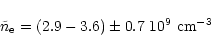
We estimated the effective radius of the H II nebula to be
![]() during this period, and its average
electron concentration
during this period, and its average
electron concentration
![]() for
for
![]() K.
K.
(iv) Our analysis of the nebular lines revealed that the [O III]
nebula in AXPer is rather dense, having an electron density
![]() for
for
![]() K.
K.
(v) Spectra taken at the middle of the 1992.8 and 1994.7 eclipses
showed that about 60, 40 and 80% of the flux emitted in the He II
nebular [O III] and H![]() lines, respectively, has
an origin in the vicinity of the hot star - within the radius of
the stellar disk of the giant. The very different density in
the H II and [O III] emission regions, but, on
the other hand, their proximity, implies a complex structure
of the material accreted from the wind by the hot component.
lines, respectively, has
an origin in the vicinity of the hot star - within the radius of
the stellar disk of the giant. The very different density in
the H II and [O III] emission regions, but, on
the other hand, their proximity, implies a complex structure
of the material accreted from the wind by the hot component.
(vi) Analysis of the hydrogen Balmer lines showed that their profiles
are affected mainly by an absorption component arising in the neutral
portion of the giant's wind. From its position, we determined the
terminal velocity of the wind,
![]() .
The temperature of the hot star increased from
.
The temperature of the hot star increased from ![]() 115000 to
115000 to
![]() 170000K, during transition from 1992 to 1998.
170000K, during transition from 1992 to 1998.
(vii) Transition of AXPer to its nebular phase happened around
JD2450000 and lasted a short time of 30-40 days. The narrow
minima observed in the LC prior to this time drastically changed
into a very broad wave-like phase-dependent variation. This transition
was caused by dilution of the shell around the hot star, which
injected approximately of
1.5 1050 particles
(![]()
![]() )
into the ionized region.
These new emitters converted a part of the far-UV radiation of the hot
star by recombination and free-free transitions into the optical region,
where we observed it as the 0.6mag flare.
)
into the ionized region.
These new emitters converted a part of the far-UV radiation of the hot
star by recombination and free-free transitions into the optical region,
where we observed it as the 0.6mag flare.
Acknowledgements
This research was supported by the Alexander von Humboldt foundation under project SLA/1039115 and by the Slovak Academy of Sciences under grant 5038/2000. We thank Horst Drechsel for reading the manuscript and commenting on it, and Drahomír Chochol for the kind provision of the 13/10/92 spectrum secured at the Asiago Astrophysical Observatory. AS acknowledges the hospitality of the Astronomical Institute, University of Erlangen-Nürnberg, in Bamberg, and of the Capodimonte Astronomical Observatory, in Naples.
![\begin{figure}
\par\includegraphics[width=17.2cm,clip]{ms10145f5.eps} \end{figure}](/articles/aa/full/2001/07/aa10145/img44.gif)
![\begin{figure}
\par\includegraphics[width=16.6cm,clip]{ms10145f6.eps} \end{figure}](/articles/aa/full/2001/07/aa10145/img45.gif)
![\begin{figure}
\includegraphics[width=7cm,clip]{ms10145f10.eps} \end{figure}](/articles/aa/full/2001/07/aa10145/img143.gif)