A&A 366, 547-557 (2001)
DOI: 10.1051/0004-6361:20000196

Simultaneous intensive photometry and high resolution spectroscopy of $\delta$ Scuti stars

V. The high-degree modes in the pulsational content of BV Circini

L. Mantegazza - E. Poretti - F. M. Zerbi

Osservatorio Astronomico di Brera, Via E. Bianchi 46, 23807 Merate, Italy

Received 6 September 2000 / Accepted 3 November 2000

Abstract
We discuss here the pulsation properties of the $\delta$ Scuti star BV Circini on the basis of data obtained during a simultaneous photometric and spectroscopic campaign in 1996 and a spectroscopic one in 1998, and taking also advantage of the previous photometric observations by Kurtz (#!kur81!#). Nine pulsation modes were detected from photometry and thirteen from spectroscopy; five of them are in common to both techniques. The spectroscopic data give ample evidence of dramatic amplitude variations in some modes, in particular the strongest spectroscopic mode in 1998 was not detectable in 1996 data. The two dominant photometric modes (6.33 and 7.89 cd^-1) are observed on both seasons. The typing of the modes was performed by means of a simultaneous model fit of line profile and light variations. The 6.33 cd^-1photometric term is probably the fundamental radial mode, while the 7.89 cd^-1is a nonradial mode with $m\neq 0$. There are six high-degree prograde modes with an azimuthal order m ranging from -12 to -14, and also a retrograde mode with $m\sim 7$. These modes combined with the identification of the 6.33 cd^-1mode allowed us to estimate $i\sim 60^{\rm o}$for the value of the inclination of the rotation axis. An accurate evaluation of the main stellar physical parameters is also proposed as a result of the pulsational analysis.

Key words: methods: data analysis - techniques: spectroscopic - techniques: photometric - stars: individual: BV Cir - stars: oscillations - stars: variables: $\delta$ Sct

1 Introduction

Asteroseismology is knowing an increasing interest thanks to satellites which are expected to fly in the incoming years (MOST, MONS, COROT) and which will perform accurate investigations of stellar variability at the $\mu$mag level. Stars located in the lower part of the instability strip are suitable candidates to find a large quantity of excited modes, both radial and nonradial. The detailed knowledge of the pulsational properties of $\delta$ Sct stars can help in the preparation of the scientific background of these missions; a review of the photometric properties of these variable stars is given by Poretti (2000). The main difficulty in their investigation is the typing of the excited modes, i.e. classifying the oscillations in terms of quantum numbers $n,\; \ell$ and m. To proceed on this way, we started an observational project combining photometric and spectroscopic techniques at the European Southern Observatory. In this paper we supply the last result, after those on FG Vir (Mantegazza et al. 1994), X Cae (Mantegazza & Poretti 1996; Mantegazza et al. 2000) and HD 2724 (Mantegazza & Poretti 1999).

BV Circini $\equiv$ HD 132209 was discovered to be a $\delta$ Scuti variable star by Kurtz (1981). He detected four pulsation modes from the frequency analysis of 18 nights of observations in the B and V colours in 1980. The author also pointed out that these modes did not provide a complete description of the stellar variability. The strongest term at 6.328 cd^-1 was suggested to be the radial fundamental mode. Since the star is rather bright (V=6.56) and its light variations are quite large ( $\Delta V>0.1$ mag), we decided to include it among our targets.

2 Physical parameters

The stellar physical parameters can be estimated independently by means of the $uvby\beta$ and Geneva colour indices and related calibrations. They are required for fitting the line profile variations and are useful for discussing the pulsation properties.

The Moon & Dworetsky (1985) calibration applied to Hauck & Mermilliod's $uvby\beta$data supplies $T_{\rm eff}=7330\pm30$ K and $\log g=3.58\pm 0.06$(this estimate also includes the correction for metallicity effects as derived by Dworetsky & Moon 1986). The recent calibration of Geneva photometric indices by Kunzli et al. (1997) applied to the data by Rufener (1988) supplies $T_{\rm eff}=7185\pm62$ K and $\log g=3.95\pm 0.10$. The discrepancy in the value of the temperature is negligible since models are marginally affected by small temperature differences. In the following an average value of $T_{\rm eff}=7260\pm100$ K will be adopted.

The disagreement on $\log g$ deserves further investigation in the future, since it has also been found for X Cae (Mantegazza et al. 2000). From some tests made on other $\delta$ Sct stars, the $\log g$ values derived from Geneva photometry seem to be always higher than those derived from $uvby\beta$photometry, even if usually with a lesser extent than here. In the case of BV Cir, the HIPPARCOS parallax measurement ( $7.85\pm0.60$ mas) offers us the possibility to solve the matter. From this parallax and the interstellar reddening estimate supplied by the $uvby\beta$ indices ( E(b-y)=0.022, and thus A_V=0.095), we derive $M_V=0.94\pm0.17$ and therefore $M_{\rm bol}=0.97$ (BC=+0.035, Flower 1996). Finally, from the photometric temperature and the HIPPARCOS luminosity, we get $R=3.59\pm 0.30$ $R_{\odot}$. BV Cir is then an evolved $\delta$ Scuti star, located in the middle of the instability strip, slightly shifted toward the cold border.

According to the theoretical models by Schaller et al. (1992) a mass of $2.0\pm0.1~ M_{\odot}$ can correspond to such temperature and luminosity; finally, by combining this with the radius estimate we get $\log g=3.62\pm 0.09$ in nice agreement with the estimate from the Moon & Dworetsky (1985) calibration.

3 Frequency analysis of Kurtz's (1981) photometric data

Since the solution proposed by Kurtz (1981) did not give a fully satisfactory fit of the observations, we decided to analyze his data with the least-squares power spectrum technique, which has been widely used by us in a lot of papers and has proved to be rather efficient in analysing multi-periodic time-series (e.g. Mantegazza et al. 2000).

Both B and V datasets were independently analyzed and the results are summarized in Table 1. Nine components were found in common between the two datasets, 8 with the same frequencies and one with an uncertainty of 1 cd^-1(9.232 cd^-1in B and 10.232 cd^-1in V). One low frequency term was detected in both datasets, but the frequency is slightly different (0.295 cd^-1in B and 0.239 cd^-1in V). Owing to the fact that the data are distributed in 5 sequential segments and were obtained with three different telescopes, this term could be due to the procedure adopted to align the differents datasets. This spurious nature can account for the quite high A_B/A_V ratio, i.e. 1.9, unlikely for a pulsation mode.

The four strongest terms are the same as detected by Kurtz (1981). We note that among the new terms, a frequency (9.901 cd^-1) is very close to a 2 cd^-1alias of the term at 7.892 cd^-1. However, it should be a real feature since each attempt to get rid of it has failed (for example by substituting the two frequencies with the intermediate alias at 8.90 cd^-1and so on).

Other terms are probably present but their unambiguous detection is problematic with the present data. There could be also variations in the amplitudes of the detected terms, as detected in the spectroscopic data (see below); since the photometric baseline spans 116 days, these variations could be appreciable, but again the data sample is inadequate to supply an unambiguous answer.

In order to get a final list of frequencies, the B and V data were put together by aligning the zero-points and rescaling the V data in order to match the B amplitudes; the resulting time-series was frequency analyzed again. This approach is the same as used by Breger et al. (1998) to study FG Vir and by Mantegazza et al. (2000) to study X Cae. The frequencies detected in this way are also listed in Table 1; the B and V amplitudes obtained by fitting the respective time-series and the rms residual are also reported.

 

 

Table 1: Reanalysis of the photometric data supplied by Kurtz (1981). The terms at 11.077 and 11.128 cd^-1were no further observed in 1996

Frequencies [cd-1]				Amplitudes [mmag]
B	V	$B\&V$		AB	AV
0.295	0.239	0.294		3.1	1.6
6.328	6.328	6.328		24.3	19.7
7.892	7.892	7.892		10.0	8.2
9.901	9.901	9.901		5.6	4.6
9.232	10.233	10.234		2.5	2.0
11.077	11.077	11.077		3.5	3.6
11.128	11.128	11.128		6.8	6.0
11.631	11.631	11.631		7.3	6.0
12.289	12.289	12.289		12.5	10.0
12.381	12.380	12.381		5.4	4.1
rms residuals				4.4	3.5

4 New photometric observations

The photometric data presented in this paper were collected during a campaign in June 1996 with the 0.5 m telescope at la Silla Observatory. During five consecutive nights 322 and 312 measurements were collected in the Strömgren v and y bands respectively. Differential photometry was performed by using HD 132249 and HD 132222 as comparison stars. These stars were used by Kurtz (1981), who found them constant at the mmag level. Due to the non-perfect atmospheric transparency during these Chilean winter nights, systematic intra-night variations were noticed in the extinction coefficient. Therefore, the data were reduced by means of the instantaneous extinction coefficient procedure (Poretti & Zerbi 1993). Nevertheless, the photometric measurements could not reach the typical level of precision for the La Silla site; the magnitude differences between the two comparison stars show a standard deviation of 6.5 mmag in y-light and 8.7 mmag in v-light.

The new observations were analyzed with the same approach adopted for the Kurtz (1981) data: the v and y measurements were first frequency analyzed separately and then were merged together. The detected frequencies are listed in the first 3 columns of Table 2. We notice that the spectral resolution of this dataset, 0.2 cd^-1, is consistently lower than that of the 1980 dataset. In the 4th column the corresponding frequencies of Table 1 are reported for comparison purposes. The frequencies at 6.328 and 7.892 cd^-1that were dominant in the 1980 data are still present in the new photometry still with a dominant character. A number of other terms such as 9.901, 11.631, 12.289, 12.381 cd^-1were also confirmed in the new photometry while the term at 10.234 cd^-1 presented some aliasing uncertainty. The terms at 11.077 and 11.128 cd^-1were not recovered in the 1996 dataset; as we shall see later, they were not detected in the spectroscopic analysis too. Also in our dataset low frequency terms are observed, at values (0.36 cd^-1and its alias 0.64 cd^-1) different from those observed in Kurtz's data (0.29 cd^-1): this difference can be accounted for the worst frequency resolution, but it is greater than that observed for other terms (see Table 2). Moreover, the power spectrum of the measurements between the two comparison stars shows increased noise at f<1 cd^-1, strongly supporting a spurious nature of the detected peaks.

	Figure 1: Light curves obtained at ESO in the y-light. The fit is calculated by using the parameters listed in Table 2
Open with DEXTER

Amplitudes in the v and y bands were derived by fitting the respective data adopting the Kurtz values for the frequencies, which are more accurate because of the longer baseline. Figure 1 shows the fit of the measurements in the y-band. By comparing the Vamplitudes of Kurtz's (1981) data with those of the present ones it appears that most of the terms have comparable values. This is not true for the 10.23 cd^-1term, much stronger in the recent data. However, this term is not well resolved from the alias at 2 cd^-1of the 12.29 cd^-1term and therefore this effect could be spurious.

 

 

Table 2: Frequency analysis of the new photometric data

Frequencies [cd-1]					Amplitudes [mmag]
v	y	$v\&y$	$B\&V$		Av	Ay
0.64	0.36	0.65	--		4.8	3.9
6.33	6.33	6.33	6.328		28.2	19.3
7.88	7.88	7.87	7.892		16.0	10.3
--	9.93	9.94	9.901		6.9	5.5
10.28	9.23	9.27	10.234		9.2	7.1
11.69	11.61	11.63	11.631		8.7	5.8
--	11.25	12.29	12.289		10.5	7.3
11.38	13.42	12.36	12.381		7.3	5.4
	rms residuals				7.2	5.4

5 Spectroscopic observations and data processing

The spectroscopic observations were performed during two runs in 1996 and 1998 at La Silla Observatory (ESO) with the Coudé Echelle Spectrograph attached to the Coudé Auxiliary Telescope (1.4 m).

The first run (6 consecutive nights, June 18-24, 1996) was performed in Remote Control Mode from Garching with the CES configured in the blue path with the long camera and the CCD #38. The reciprocal dispersion was 0.018 Å pix^-1 with an effective resolution of about 54000, and the useful spectral region ranged from 4482 to 4532 Å. The weather conditions were not always optimal and, to get an adequate S/N, the integration times ranged between 12 to 25 min. 118 useful spectrograms were gathered; they monitor the star variability for about 38 hours (duty cycle of about 30$\%$) and on a baseline of 5.2 days.

The second run (12 consecutive nights, June 7-19, 1998) was performed from La Silla with the same CCD and blue path, but with the very-long camera. The reciprocal dispersion was of 0.0075 Å pix^-1 with an effective resolution of about 51000. The useful spectral region ranged from 4498 to 4517 Å. Integration times were of 15 min and a total of 156 useful spectrograms were obtained during 9 nights, corresponding to about 48 hours of stellar monitoring (duty cycle about 18$\%$) on a baseline of 11.3 days.

The data reduction was performed using the MIDAS package developed at ESO. The spectrograms have been normalized by means of internal quartz lamp flat fields, and calibrated into wavelengths by means of a thorium lamp.

The spectrograms of each run have then been averaged and some windows on the continuum were selected in the very high S/N mean spectra. The individual spectrograms have been normalized to the continuum by fitting a 3rd degree polynomial to these windows for the first run set (longer spectral range) and a 2nd degree polynomial for the second run set (shorter spectral range).

Finally the spectra have been shifted in order to remove the observer's motion (Earth's rotation and revolution). The spectrograms were rebinned with a step of 0.04 Å  (average of 2 original pixels) for the first season data and of 0.035 Å  (average of 5 original pixels) for the second one. This step allows us to save the effective resolution according to the Nyquist criterion, and not to have too many pixels to analyze.

Due to the relatively high projected rotation velocity (see below), only the Fe  II line at 4508.3 Å  is completely free from blends of adjacent features, and therefore was the only line suitable to study line profile variations.

The mean standard deviation of the pixels belonging to the continuum allows an estimation of the S/N of the spectrograms. The resulting average value at the continuum level is about 257 for the first season data and 251 for the second one.

A non-linear least-squares fit of a rotationally broadened Gaussian profile to the average line profiles of the two seasons allows us to get very similar estimates of the projected rotational velocity and the intrinsic width of the 4508 Å  line. We get $v\sin i=96.5\pm 1.0$ kms^-1and $W_i=12.5\pm 0.5$ kms^-1, respectively.

6 Analysis of spectroscopic variations

6.1 Radial velocities and the second moment of the line profile

Radial velocities were derived by the computation of the instantaneous line barycentre (i.e. they coincide with the first moment of the line profile, Balona 1986). They were derived for both datesets and the two resulting timeseries were analyzed by the same least-squares technique adopted for the light curve analysis. The amplitudes of radial velocity variations are rather small, not exceeding 5 km s^-1peak to peak; the accuracy of these data is 0.6-0.7 km s^-1as estimated from the white noise level. Because of this, only the 6.33 cd^-1can be detected unambiguously in both datasets. Its semi-amplitude is the same within the uncertainties in both seasons: $1.3\pm0.1~$kms^-1. The fit of the radial velocity data with the other photometrically dominant frequencies shows that these terms should have amplitudes of the order of 0.5 km s^-1or less. The analysis of the second moment supplies again the same result for both seasons: only one mode is clearly discernible, but it is the 7.89 cd^-1, not the 6.33 cd^-1mode. Forcing the fit of the 6.33 cd^-1 term to the data we get a negligible amplitude. The conclusion is that the 6.33 cd^-1mode, which is also the photometrically dominant term, is axisymmetric (m=0); on the contrary the 7.89 cd^-1mode should have $m\neq 0$.

6.2 Analysis of the line profile variations

The variations of the shape of the line profiles was studied by means of the pixel by pixel analysis. A detailed description of this approach was made by Mantegazza & Poretti (1999) and by Mantegazza (2000). In particular Fig. 6 of the second paper shows the pixel by pixel least-squares power spectrum relative to the Fe  II 4508 Å  line of BV Cir as derived from the 1998 data, where it is apparent that there is a significant contribution to the line profile variations in the whole frequency range (from 1 to 20 cd^-1).

	Figure 2: Least-squares global power spectra of the line profile variations of the 4508 Å  line. Left: 1996 data; right: 1998 data. Upper panels: spectra of the signal contained in the data. Lower panels: residual spectra after considering all the detected terms. The reduction factors refer to the initial data variance of the respective season both in the upper and lower panels
Open with DEXTER

The frequencies detected for the two datasets with this technique are listed in order of increasing frequency in Table 3. Not all the terms were detected in both seasons; in particular the dominant term in the 1998 data (17.28 cd^-1) was not seen in the 1996 ones. The upper panels of Fig. 2 show all the signal contained in the data, while the bottom panels show the signal left after considering all the detected terms. In the 2nd and 3rd columns of Table 3 we report the mean square amplitudes across the line profile of the detected terms for the 1996 and 1998 data respectively. These quantities are expressed in square units of the local continuum of the stellar spectrum. Due to the high number of excited modes and to the complexity of the spectral window it cannot be ruled out that some of the detected frequencies could be 1 cd^-1aliases of the true ones. We can be more confident on terms which have been independently detected in both seasons and/or in the photometric data.

 

 

Table 3: Detected modes by pixel by pixel least-squares frequency analysis of high-resolution spectrograms. The photometric counterparts are also reported

Freq.		Power		Photom.
[cd-1]		1996	1998	[cd-1]
0.65		2.88	3.28	0.65
1.48		4.02	2.88	--
2.22		--	3.08	--
6.33		3.42	2.42	6.328
7.89		3.40	3.55	7.892
9.90		--	2.85	9.901
11.63		3.11	3.40	11.631
(13.43)		3.18	--	12.381
13.85		9.04	10.07	--
14.34		4.41	2.87	--
14.95		7.97	7.03	--
15.80		--	3.86	--
16.44		--	6.74	--
17.28		--	12.87	--

Fourteen terms were detected out of which seven were present in both seasons. Moreover six terms have an independent photometric detection: 0.65, 6.33, 7.89, 9.90, 11.63 and 13.43 cd^-1. The last value probably corresponds to the 1 cd^-1alias of the photometric value of 12.38 cd^-1and in the following we shall adopt this photometric value. The nature of the low-frequency terms is discussed in Sect. 6.4.

An independent check of these detections can be performed with the CLEAN algorithm (Roberts et al. 1987) generalized to study line profile variations (see for example Bossi et al. 1998; De Mey et al. 1998). Such an approach is complementary to the previous one because the selection of the peaks is completely automatic, i.e. free from human judgement, with the consequent merits and defects. Among the merits the major one is the absence of human intervention: indeed any time we select a known constituent and add it to the least-squares solution we intervene on the representation of the signal thus conditioning to some extent the next procedure. Among the defects the major one is that CLEAN is in condition to make a reliable distinction between a true signal and an alias only when the spectral window is of very good quality. For this reason the procedure we adopted in the past on similar analyses was to put more reliability on the least-squares analysis and use CLEAN only as a cross-check. Moreover, for sake of clarity, we prefer to use the CLEAN power spectra to present the frequency content of the data.

The results of the CLEAN analysis are shown in the two panels of Fig. 3. By comparing this figure with Table 3 we can see that there are no great differences with the least-squares technique and that both techniques agree on several detections. Two different alias identifications are observed: the 0.65 and 0.35 cd^-1peaks, the 14.94 and 13.94 cd^-1peaks. Moreover, in the 1998 data the 12.87 and 13.85 cd^-1peaks are related to the same term. It is also possible to see that the peaks of the 1998 data are narrower than those of the 1996 data because of the longer baseline; the same fact can be appreciated with the least-squares power spectra (Fig. 2).

The comparison with the least-squares analysis confirms most of the terms (0.65, 1.46, 2.22, 6.33, 7.89, 9.92, 11.63, 14.34 and 17.28 cd^-1) and allows us to prefer the 14.94 and 13.85 cd^-1terms to their aliases.

As regards the terms with frequencies around 16.2-16.5 cd^-1, both CLEAN and the least-squares technique confirm the difference between the 1996 (no significant term detected in this region) and 1998 (a bunch of detected terms) datasets. The least-squares technique seems to explain the signal in this region in a simplest way (a unique term, rather than the three suggested by CLEAN). Moreover, CLEAN did not reveal clearly the 15.80 and 12.38 cd^-1terms. These small discrepancies can be accounted for by a noise effect and bad spectral window. In the following analysis we shall use the terms identified by means of the least-squares approach.

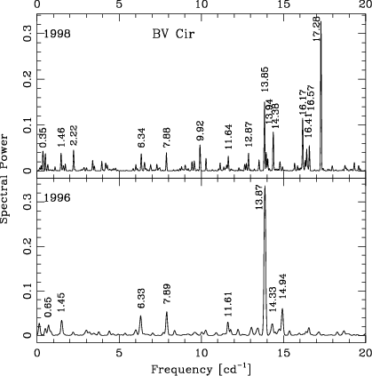	Figure 3: Average CLEAN power spectra of the line profile variations across the Fe  II 4508 Å line. The frequencies of the main peaks are given in the labels. Lower panel: 1996 data; upper panel: 1998 data
Open with DEXTER

Figure 4: Behaviours of phases across the line profile of the Fe  II 4508 Å line of the terms detected with the least-squares power spectrum analysis both in the 1996 and the 1998 data. The phases are in degrees (each tickmark corresponds to $50^{\rm o}$). The thin horizontal line in each panel gives the zeropoint level. The line profile is measured in Doppler velocities: the centre of the line defines the zeropoint. The frequency of each mode is written on the top of each panel. The doubtful pulsational nature of the 0.65 cd-1term is discussed in the text

Open with DEXTER

	Figure 5: Same as in the previous figure but relative to the modes detected in one dataset only: 12.38 cd-1and 14.34 cd-1were detected in the 1996 data, the others in the 1998 ones. The doubtful pulsational nature of the 2.22 cd-1term is discussed in the text
Open with DEXTER

In particular, we don't put particular confidence on the low-frequency terms, except for the 1.48 cd^-1term. The other terms (0.65 and its alias 0.35 cd^-1, the 2.22 cd^-1) are considered to be spurious ones (see Sect. 6.4).

The behaviours of phases across the line profile of the modes adopted for further analysis are shown in Fig. 4 for the 8 modes detected in the spectra of both seasons and in Fig. 5 for those detected in one dataset only. The behaviour of the 9.901 cd^-1term is puzzling. It was observed photometrically in 1980 and 1996. On this latter occasion, there was no significant spectroscopic counterpart (see lower panel of Fig. 3): the spectroscopic amplitude may be undetectable because the mode had quite a small photometric amplitude. Moreover, owing to the modest frequency resolution, its power could have been transferred via the 2 cd^-1 alias to the stronger 7.89 cd^-1mode. The frequency resolution is better in the 1998 data and the 9.901 cd^-1term was clearly detected, maybe thanks to an increased amplitude; unfortunately, we do not have photometric data with which to check this possibility. Therefore, we decided to consider a 9.90 cd^-1term in the analysis of the 1996 spectroscopic data also.

The behaviour of the phases across the line profile gives already some hints about the nature of a few of the detected modes. For instance the phases of the 13.85, 14.34, 14.95, 15.80, 16.44 and 17.28 cd^-1modes have the typical signature of high-degree prograde modes. The behaviour of the phases of the 1.48 cd^-1term is interesting because it is typical of a retrograde mode.

6.3 Mode identification: The technique

It is possible to try to estimate the $\ell$, m parameters of the detected modes by a model which fits the variations induced on the line profile shape. The technique adopted to separate the contributions of the different modes to the global observed line profile variations and to fit them is described in Mantegazza et al. (2000) and Mantegazza (2000). The theoretical line profile variations are computed according to the model developed by Balona (1987), by means of his LNPROF routine. If simultaneous light variations are available it is possible to fit them with the same model at the same time, and in this case a more accurate typing of the mode can be proposed, since we can constrain at the same time both the velocity fields and the flux variations. The best fitting modes are selected according to a "discriminant'' whose value defines the goodness with which the candidate mode reproduces the variations of the line profile and of the light (if available) of the detected frequency term. For some modes the discriminant is also sensitive to the inclination of the rotational axis, and therefore if several modes are detected it is possible to build a total discriminant (the sum of the individual ones) as a function of inclination angle i. The minimum of this function can in principle fix this parameter.

In the case of BV Cir only the 1996 data have simultaneous light and spectroscopic observations and therefore only these data can be used to perform a simultaneous fit of both quantities and hence to constrain velocity and flux variations.

	Figure 6: Discriminants of the 1.48 cd-1mode as a function of the azimuthal order m computed from the 1996 (solid lines) and 1998 (dashed lines) data. These values are relative to $i=55^{\rm o}$ and $\ell =m$. But the discriminants are rather insensitive to i and are comparable for any $\ell \geq m$
Open with DEXTER

6.4 Low frequency modes

Three terms were observed at low frequencies: 0.65, 1.48 and 2.22 cd^-1. The attempts to fit 0.65 and 2.22 cd^-1 were fruitless and no meaningful identification was possible. The phase diagrams of 0.65 (Fig. 4, left panel of the upper row) and 2.22 cd^-1(Fig. 5, left panel of the upper row) terms look like a scattered plot, without any discernible trend. This result supports our hypothesis that these terms are spurious effects in the analysis. It can be argued that the 0.65 cd^-1term is found both in the spectroscopic and in the photometric datasets, which are independent from each other. However, there are other peaks in this frequency region having similar amplitudes (see Fig. 3) and therefore the numeric coincidence can be considered as merely casual. We again remind the reader that in the photometric analysis also there are many doubts on the reality of the 0.65 cd^-1term. Therefore, in the discussion, we prefer not to consider the 0.65 and 2.22 cd^-1terms as pulsational modes, even if some uncertainties are left, especially on the former.

Figure 7: Behaviours of the discriminant of the best fitting modes versus the inclination for the terms detected both spectroscopically and photometrically. Left panels: discriminants computed by simultaneously fitting line profile and light variations in the 1996 season. Central panels: discriminant computed by fitting line profile variations in the 1996 data only. Right panels: discriminants computed by fitting line profile variations in the 1998 data. The panels of the same line concern the same term whose frequency is reported in the leftmost panel

Open with DEXTER

On the contrary the term at 1.48 cd^-1, which has been observed in both seasons, and whose phase diagrams clearly show that it is a retrograde mode, supplied useful discriminants. As is also evident from its phase diagrams (Fig. 4, right panel of the upper row) it is retrograde and has a rather high degree, and as in the case of the prograde mode the discriminant is rather insensitive to the inclination and to the $\ell$ degree. The derived values from the two datasets are shown in Fig. 6. The 1998 discriminant has a lower depth than the 1996 one because in that season the S/N was lower. In any case we can estimate m=7 or 8.

Such modes are rarely observed in $\delta$Scuti stars, and often their detection is rather ambiguous, but in this case the evidence is remarkable and is independently shown by the two datasets (Fig. 4). This typing constitutes a warning about the identification of a low-frequency terms as a g-mode, since a p-mode can assume these values in the observer's reference frame.

6.5 Modes with spectroscopic and photometric detections

The identification of the modes which were independently detected both by photometry and spectroscopy was performed looking for all the possible $\ell,m$ combinations up to $\ell=4$and with inclinations of the rotation axis between 20 and 90 degrees (the lower limit was fixed considering that the star reaches the break-up velocity at about $i=17^{\rm o}$). The main results are shown in Fig. 7 where the horizontal panels belong to the same mode whose frequency is reported in the leftmost panel. In each panel the behaviours of the discriminants versus the inclinations of the best fitting modes are reported. Each mode is identified by a different colour. Since in the 1998 season we have no photometric data, in order to allow a comparison of the results the 1996 data were analyzed fitting simultaneously line profile and light variations (left panels) and only line profile variations (central panels). The panels on the right contain the discriminant computed from the 1998 spectroscopic data. In the first case the models allowed for both velocity and flux variations, while in the second case only velocity variations were considered. In the 1998 data the 12.38 cd^-1term was not detected and therefore the corresponding panel is missing. The simultaneous fitting of velocity and flux variations made the results shown in the leftmost panels more reliable. Those in the other two panels are useful only to check how reasonable it is to neglect flux variations to model line profile variations (and hence if we can avoid getting simultaneous light and spectroscopic data) and the consistency between the two seasons' data. The general conclusion is that the agreement between the best fitting modes in the two seasons' data is reasonable because the best fitting modes are the same, with a few exceptions. However we can see that by fitting line profile variations only we tend to assign a higher degree to the detected modes. The light curves play a decisive role in the mode typing since the photometric amplitude is very sensitive to the cancellation effects originated by the high-degree modes. For instance for the 6.33 cd^-1term the possibility of identifying it as 3,0is completely ruled out if we also take into account light variations.

As regards possible identification, we can give reasonable estimates for two terms only. The terms at 9.91, 11.63, and 12.38 cd^-1are the more uncertain since many modes supply comparable results. The term at 6.33 cd^-1is certaintly axissymmetric (all the proposed identifications have m=0) and its most probable identification is $\ell=0$, m=0, unless the star is seen almost exactly equator-on. In this case $\ell=2$, m=0 could also be possible. The term at 7.89 cd^-1has $\ell=1$, m=-1 or $\ell=2$, m=-1 as the most probable identifications, although we cannot completely rule out the possibility $\ell=2$, m=-2.

	Figure 8: Discriminants of the six high degree prograde modes as a function of the azimuthal order m computed from the 1996 (dashed lines) and 1998 (solid lines) data. These values are relative to $i=55^{\rm o}$ and $\ell =-m$. But the discriminants are rather insensitive to i and are comparable for any $\ell\geq\;\mid m\mid$
Open with DEXTER

Because of the mode involved, the present discriminants do not help very much to decide on the most probable inclination of the rotational axis, which however will be constrained on the basis of different considerations later.

6.6 High degree prograde modes

Six of the detected terms belong to this group: 13.85 and 14.95 cd^-1(which were detected both in the 1996 and in the 1998 data), 14.34 cd^-1(which was detected in the 1996 data) and 15.80, 16.44 and 17.28 cd^-1(which were detected in the 1998 data). In order to fit the line profile variations produced by these terms all the prograde modes with $5\leq \ell \leq 20$ were explored, either taking into account flux variations or not. These high-$\ell$ modes are not very sensitive to flux variations. In turn, line profile variations are rather insensitive to the inclination and to the $\ell$ degree, while they were strongly dependent upon the azimuthal order. Figure 8 shows the discriminant of these six terms as a function of m and computed for $i=55^{\rm o}$ and $\ell=\;\mid m\mid$. However as was said above the inclination is rather unimportant, as for a fixed mode the discriminant is flat at minimum and increases appreciably only for $i \leq 35^{\rm o}$. In Fig. 8 the solid lines indicate the discriminants derived from the 1998 data while the dashed lines indicate those obtained from the 1996 data, and they are in agreement. From Fig. 8 we can also estimate the m values reported in Table 4.

As an example of how the fits of the models to the observational quantities look we show in Fig. 9 the behaviour of the amplitude and phase across the line profile of the 17.28 cd^-1mode with the best fitting solutions for $\ell=12, m=-12$ (dashed lines) and $\ell=13, m=-13$ (dotted lines).

	Figure 9: Behaviour of amplitude (solid line upper panel) and phase (dots, lower panel) of the 17.28 cd-1term across the line profile and their best fits with $\ell =-m=12$ (dashed lines) and $\ell =-m=13$ (dotted lines)
Open with DEXTER

 

 

Table 4: Detection (Y: positive; N: negative) and typings of the pulsation modes observed in the photometric (P, 1980 and 1996) and spectroscopic (S, 1996 and 1998) datasets of BV Cir. No mode identification is possible for the modes detected only photometrically (lower panel)

Freq.	Tech.	Typing		Detection
[cd-1]			1996	1998
1.48	S	m=7 or 8	Y	Y
6.33	S P	$\ell=0$, m=0	Y	Y
7.89	S P	$\ell=1$ or 2, m= -1 or -2	Y	Y
9.91	S P	$0\leq\ell\leq3, m>0$	Y	Y
11.63	S P	$\ell=2\pm1$, m=-1 or -2	Y	Y
12.38	S P	$-1\leq\ell\leq3, m<1, m\neq0$	Y	N
13.85	S	m= -12 or -13	Y	Y
14.34	S	m= -13	Y	Y
14.95	S	m= -14	Y	Y
15.80	S	m= -13	N	Y
16.44	S	m= -12	N	Y
17.28	S	m= -12 or -13	N	Y
			1980	1996
10.23	P		Y	Y
12.29	P		Y	Y
11.077	P		Y	N
11.128	P		Y	N

7 Discussion and conclusions

BV Circini has a lot of excited pulsation modes with observed frequencies ranging from low to high values. Nine frequencies were detected from photometric data (1980 and 1996) and 13 from spectroscopic (1996 and 1998) ones, 5 of them are in common in both datasets. The amplitudes of some modes are dramatically changing and this is particularly evident from the two spectroscopic datasets, in particular the strongest spectroscopic mode in the 1998 data at 17.28 cd^-1, was not detectable in the previous dataset.

Six of the detected modes are high azimuthal order prograde modes with $-14\leq m \leq -12$ and one is retrograde with m=7 or 8. For only two of the modes detected by simultaneous photometry and spectroscopy it has been possible to suggest a complete $(\ell, m)$ identification, while better S/N spectroscopic data are needed for the others. The two identified modes are the one at 6.33 cd^-1(the photometric dominant mode), which can be identified as the $\ell=0$ (radial mode). The other is the one at 7.89 cd^-1which is a low degree prograde mode with $\ell=1$ or 2 and m=-1. The proposed typings of the pulsation modes of BV Cir are summarized in Table 4.

By using the physical parameters computed in Sect. 2 we can evaluate the pulsation constant of the 6.33 cd^-1mode, i.e. $Q=0.032\pm0.005$ d. Therefore, this mode is probably the radial fundamental in agreement with the suggestion by Kurtz (1981). If we take this result for granted, we can use this information to narrow the uncertainties on some physical parameters. In fact, assuming for this mode the theoretical value of $Q=0.033\pm 0.001$ d as pulsation constant, we get from its definition $\overline{\rho}/\overline{\rho}_{\odot}=0.044\pm 0.003$ and also $\log g=3.63\pm0.04$. Moreover if we combine the mean density with the radius estimate we get $M=2.04\pm 0.12~ M_{\odot}$, again in excellent agreement with the value derived from the evolutionary models (see Sect. 2).

Hence by comparing the information from pulsation properties (as derived from our analysis), HIPPARCOS parallax and effective temperature (as derived from multicolour photometry), we determined physical parameters which are perfectly consistent (Table 5.)

We have remarked in the previous section that the discriminants of the detected modes are not particularly sensitive to the inclination of the rotation axis. However we can constrain this value using the azimuthal orders derived for the high degree modes and the fact that the 6.33 cd^-1 mode is the radial fundamental, because in this case their frequencies in the stellar reference frame should be larger than the radial fundamental one. Among the prograde modes the critical one is the 13.85 cd^-1, which with $m=-12.5\pm 1$ imposes $i\geq 62^{\rm o}\pm10^{\rm o}$, while the 1.48 cd^-1with $m=7.5\pm1$ gives $i\leq 56^{\rm o}\pm 12^{\rm o}$. By combining the two results we obtain $i\sim 60^{\rm o}$. Consequently the equatorial rotation velocity is about 111 kms^-1 and the rotation frequency $\Omega$ about 0.61 rev d^-1.

 

 

Table 5: Basic physical parameters of BV Cir

Parameter	Estimated value
Mass	$2.04\pm 0.12~ M_{\odot}$
Effective temperature	$7260\pm100^{\rm o}\;$K
Absolute bolometric magnitude	$0.97\pm 0.17$
$\log g$	$3.63\pm0.04$
Radius	$3.59\pm0.30~ R_{\odot}$
Equatorial rotational velocity	$111\pm 12$ kms-1
Rotational frequency	$0.61\pm0.07$ d-1

Let us finally deal with a few considerations about the technique to fit line profile variations. We have seen that in order to get an unambiguous discrimination between the possible identifications we need data with a rather high S/N. The present data, with a S/N of the order of 250, supply useful information for the strongest spectroscopic terms only. Since the observed amplitudes are typical of $\delta$ Scuti stars, it is not unreasonable to believe that, in order to do a good job, data with a S/N of 500 or better could be necessary.

We have also explored the difference between fitting line profile variations considering velocity fields only or taking also into account flux variations. We have seen that in the first case we tend to overweight the higher degree modes when we try to identify low degree modes. For these modes it is therefore important to consider flux variations too, and in this case, in order to properly constrain the fitted model, it is necessary to have simultaneous light variations.

Acknowledgements

The authors wish to thank D. Kurtz for kindly putting his data at their disposal and Jacques Vialle for checking the English form of the manuscript.

References

 

• Bossi, M., Mantegazza, L., & Nuñez, N. S. 1998, A&A, 336, 518 In the text NASA ADS  
• Balona, L. 1986, MNRAS, 220, 647 In the text NASA ADS  
• Balona, L. 1987, MNRAS, 224, 41 In the text NASA ADS  
• Breger, M., Zima, W., Handler, G., et al. 1998, A&A, 331, 271 In the text NASA ADS  
• De Mey, K., Daems, K., & Sterken, C. 1998, A&A, 336, 327 In the text  
• Dworetsky, M. M., & Moon, T. T. 1986, MNRAS, 220, 787 In the text NASA ADS  
• Flower, P. J. 1996 ApJ, 469, 355 In the text NASA ADS  
• Hauck, B., & Mermilliod, M. 1990, A&AS, 40, 1 NASA ADS  
• Kunzli, M., North, P., Kurucz, R. L., & Nicolet, B. 1997, A&AS, 122, 51 In the text NASA ADS  
• Kurtz, D. W. 1981, MNRAS, 196, 53 In the text NASA ADS  
• Mantegazza, L. 2000, in Delta Scuti and Related Stars, ed. M. Breger, & M. H. Montgomery, ASP Conf. Ser., 210, 138 In the text  
• Mantegazza, L., & Poretti, E. 1996, A&A, 312, 855 In the text NASA ADS  
• Mantegazza, L., & Poretti, E. 1999, A&A, 348, 139 In the text NASA ADS  
• Mantegazza, L., Poretti, E., & Bossi, M. 1994, A&A, 287, 95 NASA ADS  
• Mantegazza, L., Zerbi, F. M., & Sacchi, A. 2000, A&A, 354, 112 In the text NASA ADS  
• Moon, T. T., & Dworetsky, M. M. 1985, MNRAS, 217, 305 In the text NASA ADS  
• Poretti, E. 2000, in Delta Scuti and Related Stars, ed. M. Breger, & M. H. Montgomery, ASP Conf. Ser., 210, 45 In the text  
• Poretti, E., & Zerbi, F. M. 1993, A&A, 268, 369 In the text NASA ADS  
• Roberts, D. H., Lehar, J., & Dreher, J. W. 1987, AJ, 93, 698 In the text  
• Rufener, F. 1988, Catalogue of stars measured in the Genève Observatory Photometric System, Genève Obs. In the text  
• Schaller, G., Schaerer, D., Meynet, G., & Maeder, A. 1992, A&AS, 96, 269 In the text NASA ADS