A&A 366, 317-325 (2001)
DOI: 10.1051/0004-6361:20000088

Multi-resolution wavelet analysis of high time resolution millimeter wavelength observations of solar bursts

C. G. Giménez de Castro¹ - J.-P. Raulin¹ - C. H. Mandrini² - P. Kaufmann¹ - A. Magun³

1 - CRAAE: (Mackenzie, INPE, USP, UNICAMP), Instituto Presbiteriano Mackenzie, Rua de Consolação 896, 01302-000 S. Paulo, SP, Brazil
2 - Instituto de Astronomía y Física del Espacio, CC 67, Suc. 28, 1428 Buenos Aires, Argentina
3 - Institute of Applied Physics, Division of Solar Observations, University of Bern, Sidlestrasse 5, 3012 Bern, Switzerland

Received 4 January 1999 / Accepted 28 September 2000

Abstract
By means of the wavelet representation of multi-resolution analysis, we study millimeter wavelength (mm-w) radio solar bursts obtained at 48 GHz with high time resolution ($\le$8 ms); observed at Itapetinga (Brazil). The multi-resolution analysis decomposes the signal locally both in time and in frequency, allowing us to identify the different temporal structures which underlie the flux density time series and the transient phenomena characteristic of solar bursts. The analysis was applied to the flux time profile of four solar bursts observed at a mm-w, studying separately the pre-flare, impulsive and post-flare phases when possible. We find that a wide range of time scales contributes to the radio flux. The minimum time scale found for the impulsive phase is 32 ms, after which the noise dominates the emission; the maximum is 8 s. Pre- and post-flare phases have a minimum time scale of 256 ms and a maximum between 1 to 8 s. Multi-resolution "spectral indexes'', which are a measure of the self-similar behavior of the signal, are in some cases bigger for the impulsive phase than for the pre- and post-flare phases. We find that as the flux becomes higher the contribution from shorter time scales is enhanced.

Key words: Sun: flares - Sun: radio radiation - methods: data analysis

1 Introduction

Solar burst observations present an enormous challenge for time series analysis because they show structures which may be discrete, random or quasi-periodic in nature, suggesting the superposition of many different transient phenomena over a wide time scale range. Since the pioneering works of Frost (1969) and van Beek et al. (1974), it was proposed that bursts are built up with what were originally called, in X-rays, the Elementary Flare Bursts (EFB) by de Jager & de Jonge (1978). Similarly at microwaves, Kaufmann et al. (1980) later extended this concept to smaller time scales, adding a quasi-quantization hypothesis. The existence of elementary spatial scales, and the fragmentation of the energy release, may also be inferred from interpretation of statistical distributions of solar events at X-ray and radio-wavelengths (Kaufmann et al. 1978; Lu & Hamilton 1991). Unfortunately, the sensitivity of present telescopes and X-ray detectors does not always allow the observation of the manifestations of the smallest energy releases, from which we can infer the elementary scales.

 

 

Table 1: Spectral index, $\alpha _{\rm MRA}$, and limit scale for different phases and different events. The uncertainties in $\alpha _{\rm MRA}$ are computed from the mean deviation between the fitted curve and the computed value

Event	Time Resolution	Phase	Start	End	Duration	$\alpha _{\rm MRA}$	Limit Scale
	(ms)		(UT)	(UT)	(s)		(ms)
A: 1990 Dec. 30 1318 UT	1	Impulsive	13:18:42	13:18:58	16.384	$3.20 \pm 0.21$	32
B: 1990 Dec. 30 1830 UT	8	Impulsive (I)	18:28:42	18:29:14	32.768	$2.31 \pm 0.07$	64
		Intermediate	18:29:17	18:29:34	16.376	-	-
		Impulsive (II)	18:29:35	18:30:08	32.768	$1.96 \pm 0.17$	64
C: 1991 Dec. 27	8	Pre-burst	17:11:47	17:16:09	262.144	$1.66 \pm 0.14$	512
		Impulsive	17:16:09	17:20:31	262.144	$1.69 \pm 0.15$	256
		Post-burst	17:20:49	17:23:00	131.072	$1.68 \pm 0.05$	256
D: 1993 Feb. 11	1	Pre-burst	18:31:02	18:31:06	4.096	$1.72 \pm 0.20$	128
		Impulsive	18:31:15	18:31:48	32.768	$3.00 \pm 0.04$	64
		Post-burst (I)	18:32:22	18:32:55	32.768	-	256
		Post-burst (II)	18:33:32	18:34:05	32.768	-	256

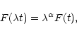
Many mathematical techniques have been employed to obtain the fundamental parameters which govern burst phenomena. The Statistical and Harmonic Analysis are among the first to have been used. In recent years, more sophisticated methods, derived from Chaos and Information Theories (Kurths & Schwarz 1994 and references therein), have also been applied successfully. Direct inspection, relating pulse counts with mean flux over equal periods of time, was explored by Kaufmann et al. (1980), Correia et al. (1995) and, more recently, by Raulin et al. (1998). This method has proven to be an excellent tool used to show the process of pile-up of elementary structures. Costa et al. (1990) have discussed techniques to identify fast structures comparing the Fourier, second derivative, and the signal subtraction smoothed burst component. Kaufmann et al. (1980) and Kaufmann (1985) have also shown that mm-w quantized energy at the origin of both small and big flares is of the same order. The limitation of this method is the overlap of the fast pulses which could not be distinguished in many cases. More analytical methods can be useful to gain insight into the presence of fast structures at higher time resolutions. The Fourier Transform could be a good candidate but, as we will show later (Sect. 3), it is not suitable for the case where transient phenomena are present.

In this work we use the multi-resolution wavelet analysis (Mallat 1989), which gives a picture both in time and in frequency of a time series, allowing us to estimate the different temporal scales involved in the different phases of bursts. We apply this method to high time resolution and sensitivity observations of solar radio bursts at 48 GHz, which are believed to be generated close to the energy release sites. Such data have a better S/N ratio in the domain of sub-seconds compared to X-ray telescopes.

This paper is organized as follows: in Sect. 2 we present the data set used, in Sect. 3 we introduce the analysis tools and refer the reader to thorough reviews. In Sect. 4 we present our findings, which are discussed in Sect. 5.

   
2 Data set

In the present work we study four bursts observed at 48 GHz, by the 13.7 m single dish radome-enclosed Itapetinga antenna with the Multibeam System (MBS), an array of 5 receivers with a Half Power Beam Width (HPBW) of about 2' at the focal plane. The MBS has been developed to achieve an accurate determination of the total flux density received, which is not altered by any displacement of the antenna with respect to the source (Giménez de Castro et al. 1999 and references therein). The absolute calibration of the flux density may have an uncertainty of less than 50%; however, it is not important for the present work since we are concerned in the relative time variations of the flux density. The total number of events which were observed at 48 GHz is small, since the antenna is not a solar dedicated instrument, and this particular receiver array was in operation from 1989 to 1993. Only a few events can be properly calibrated for a reliable analysis.

The events are described in Table 1, while their time profiles are shown in Figs. 1 and 2. When the recorded data allowed, we divided the events into different phases. The division was made in terms of the spiky (burst) and gradual (pre- and post-burst) nature of the received radiation. In the case of event A, the derived flux is too low ($\sim$0, see Fig. 1a) during the pre-burst phase to draw any reliable conclusions; therefore, we have decided not to analyze it in particular. The same occurs with the intermediate phase of event B (Fig. 1b).

	Figure 1: Time profiles at 48 GHz of the bursts analyzed. a) The derived flux density time profile for the solar burst of 1990 December 30, 1318 UT ( A). The thick horizontal line indicates the time interval studied. b) The same for the 1990 December 30, 1829 UT ( B) solar microwave burst. This event was divided in two impulsive and one intermediate phases. The intermediate phase is not analyzed
Open with DEXTER

	Figure 2: a) The derived flux density time profile for the solar burst of 1991 December 27 ( C) with its three phases. b) The same for the 1993 February 11 ( D) solar burst. The three studied intervals are also shown
Open with DEXTER

   
3 The analysis tools

The decomposition of a signal (or time series) is usually done with the Fourier Transform (FT) which uses sines and cosines as a basis. Even though they are a well accepted set of basis functions, other possibilities exist, like Bessel, Legendre etc., making the selection arbitrary. Costa et al. (1990) have demonstrated that the use of FT filters is not suitable to detect local maxima occurring during flares because it changes the shape of the signal and, thus, creates a shift in the real peak position. Because of the high frequency localization of the basis functions, the FT also loses the temporal information of the signal. Therefore, if one looks for a description also in time, a less localized set of basis functions is needed. The idea was first implemented in the Windowed Fourier Transform; however this method was also found to be inaccurate and inefficient (Kaiser 1994).

Wavelets can be used to address the previously mentioned problems. By dilations and translations of a so called mother wavelet it is possible to implement a decomposition with an adjustable interval in the frequency domain $(\Delta f)$, and in this way to catch even the episodic pulses which happen in different time scales (Daubechies 1992; Chui 1992). In a general way, we can divide wavelets into two classes: (a) continuous or nonorthogonal (CWT) and (b) discrete or orthogonal (DWT). The decision to use one or other should be taken in regard to the kind of data involved. In both cases very fast algorithms have been developed for their implementation (for the CWT see e.g. Torrence & Compo 1998, and for the DWT see e.g. Daubechies 1992; Chui 1992; Cohen & Kovacevic 1996; Strang 1989).

	Figure 3: The wavelet coefficient distribution for ${\rm scale}=-8$ and a noise amplitude equal to 0.07 s.f.u. The vertical line indicates the 99000th point and the horizontal one, its wavelet coefficient. For the sake of clarity we show the distribution near the point of interest
Open with DEXTER

In this work, we use the DWT, derived from a triangular mother wavelet which appears to be a reasonable choice as a representation of the burst pulses. Bendjoya et al. (1993) have derived an algorithm in the frame of the multi-resolution analysis (MRA) first developed by Mallat (1989). We follow the same procedure, except that our wavelets discard the redundant information.

   
4 Multi-resolution wavelet analysis

We have obtained the wavelet spectrum (WS) for each phase in the events. We note that since the MRA acts as a filter, we do not need to use any other kind of filter to denoise the data. For a time series having 2^Nelements we may have N levels or time scales (or simply, scales). The shortest one has a time resolution twice the time resolution of the original signal, the next, 4 times, and so on, increasing by a factor of two each time we change the scale. These scales represent half the period of a peak.

To estimate the uncertainty in the WS we proceeded as Torrence & Compo (1998). We created a series of 10⁵ pseudo-random signals of 2¹⁵ elements (the maximum length of a time series in our data set) with normal distribution and rms equal to the one obtained from the density flux derived from observations. For each of these pseudo-random signals we computed the WS. For each scale we took the wavelet coefficient of the middle of the interval. In this way, we produced a distribution of 10⁵ wavelet coefficients for each scale. We sorted each distribution in ascending value. Adopting the 99000th coefficient value as the uncertainty for this particular scale, we can reject with a 99% probability (1% level of significance) the hypothesis that a particular wavelet coefficient, bigger than the adopted uncertainty, originated by a normal random process. Figure 3 shows the final distribution obtained for one of the scales.

	Figure 4: a) Scalogram of the event A. Thick contours are the 1% level of significance. The other contours are drawn for 0.15, 0.3, 0.5, and 2.0 respectively. b) and c) same as a) for the first and second impulsive phases of event B
Open with DEXTER

One possible representation of the WS is the so called scalogram, which is, in fact, a 2-D plot with time as abscissa and scale as the

	Figure 5: a) Scalogram for the pre-burst phase of event C. Thick contours are the 1% level of significance. The other contours are drawn for 0.03, 0.05, 0.07, 0.09 and 0.2 respectively. b) and c): same as a) for the impulsive and post-burst phases, respectively
Open with DEXTER

ordinate; contours of equal wavelet coefficient value represent the decomposition. We show the scalogram of event A in Fig. 4a, where we interpolated the wavelet coefficients in time

	Figure 6: Scalograms of event D: a) Impulsive Phase, b) Post-burst phase (I) and c) Post-burst phase (II). Thick contours are the 1% level of significance. The other contours are drawn for 0.2, 0.3, 0.7, and 1.0 respectively
Open with DEXTER

in order to have a regular temporal grid for the whole scale range. Contours are drawn only for positive values, which reflect the peaks of the radio flux density shown in Fig. 1a. The thick contours are the 1% level of significance. The main features have a hierarchical time structure indication. Some structures appear, even at the fastest scale (2 ms). Below we discuss its possible noise nature. The two impulsive phases of event B are shown in Figs. 4b and c. They repeat the same behavior of the previous case with scales of up to 32 ms. Figures 5 and 6 show the scalograms for the other events. In general they do not show features as fast as the ones encountered in events A and B. The impulsive phase of event C (Fig. 5b) seems to have structures with scales of up to 64 ms, which are also present in the post-burst phase of the same event (Fig. 5c). We don't show the pre-burst phase of event D because it is featureless, so Fig. 6 shows only the impulsive and post-burst phases. We note that the impulsive phase (Fig. 6a) has a scale as short as 64 ms (during the interval 22-24 s), while both post-burst phases (Figs. 6b and c) show structures with longer scales.

Taking the mean square wavelet coefficient over a scale we produce a scalegram  (Scargle et al. 1993). The mathematical definition of the scalegram is as follows:

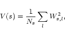$$V(s) = {1 \over N_s} \sum_l W_{s,l}^2,$$ (1)

where N_s is the total number of elements for the scale $s \in {\rm Z}$, $l \in {\rm Z}$ is the temporal index and W_s,l are the wavelet coefficients. Scalegrams are the wavelet equivalent of the FT power spectrum, and in fact, both show the same qualitative behavior for a given signal.

A time series F(t) has a self-similar behavior if:

$$F(\lambda t) = \lambda^\alpha F(t),$$ (2)

where $\alpha$ is called the similarity exponent. In that case, Scargle et al. (1993) showed that the scalegram, V(s) of F(t), should be a power law

$$V(s) \propto s^{2\alpha}.$$ (3)

We call in this work $\alpha \equiv \alpha_{\rm MRA}$ in order to specify that we obtained it from a MRA (for other ways to obtain $\alpha$ see Schwarz et al. 1998).

In order to remove the contribution of the noise in our scalegrams, we have obtained a noise scalegram with a 1% level of significance for each scale from the scalegrams of the 100000 pseudo-random time series we used before. As in Scargle et al. (1993), we corrected each obtained scalegram, subtracting the noise scalegram. But, unlike these authors, we adopted a more conservative approach and we defined the intersection between the corrected scalegram and the noise scalegram as the noise limit scale, which is the minimum scale we can identify without doubts.

Figure 7 shows the scalegram for event A. The thin solid curve is the scalegram of the whole event, the thick solid curve is the corrected scalegram, and the thick dashed curve is the scalegram of the noise. The limit scale is 32 ms. We computed the scalegram for the first 8 s (dot-dashed curve) and for the interval between 8-12 s (dashed curve) which exhibits strong pulses for scales below 32 ms in the scalogram (Fig. 4a). Both partial scalegrams have the same power law behavior for scales greater than 32 ms. However, the first 8 s interval shows a scalegram similar to the noise below the limit scale, while during the 8-12 s interval the scalegram has the same shape and slope but is well above the noise. We then conclude that a decrease in the S/N ratio occurred during the interval 8-12 s, giving rise to the features seen in the scalogram.

This event shows different power laws for different scale ranges. We consider a power law regime when three or more scales are involved. In this particular case, up to three different power laws are found; these correspond to scales ranging from 32 to 128 ms ( ${\alpha_{\rm MRA}} = 3.12 \pm 0.15$), from 256 to 1024 ms $({\alpha_{\rm MRA}} = 3.28 \pm 0.15)$ and from 2 to 8 s $({\alpha_{\rm MRA}} = 2.43 \pm 0.15)$. Taking into account that the first two values overlap we took the mean, yielding a ${\alpha_{\rm MRA}} 3.2 \pm 0.21$, which we consider characteristic for this event.

	Figure 7: Scalegrams of the derived radio flux density of the event A (Fig. 1a) The thin solid curve is the scalegram for the whole event, the dot-dashed curve for the first 8 s, the dashed curve for the interval between 8 and 12 s, the thick solid curve is the corrected scalegram, and the thick dashed curve is the noise scalegram. The vertical line shows the noise limit scale
Open with DEXTER

	Figure 8: Corrected scalegrams of the derived radio flux density of the event B (Fig. 1b) The solid curve is the corrected scalegram for the first impulsive phase, the dot-dashed curve is the second impulsive phase and the dashed curve is the noise scalegram. The vertical line shows the noise limit scale
Open with DEXTER

Figure 8 shows the corrected and noise scalegrams for the two impulsive phases of event B, which has a limit scale of 64 ms. The first impulsive phase has a power law for scales 32 to 512  ms, with ${\alpha_{\rm MRA}} = 2.31 \pm 0.07$. It has a negative slope between 512 and 1024 ms scales; afterwards the slope is always positive with the exception of the last scale. The negative slope is a clear indication of different hierarchies of structures, also seen in the scalogram (Fig. 4b). The scalegram of the second impulsive phase shows a power law regime for scales between 64 and 512 ms with $\alpha_{\rm MRA}= 1.96 \pm 0.17$, and reproduces the same hierarchical behavior of the first impulsive phase.

Figure 9 shows the scalegram of event C. The limit scale is 256 ms for the postburst and impulsive phases, while 512 ms for the preburst phase. The impulsive phase has a mean ${\alpha_{\rm MRA}} = 1.69 \pm 0.15$, for scales between 256 ms and 64 s. However, a clear variation of the slope from scales 1 to 16 s is seen, which means a smaller mean wavelet coefficient, principally for the scale 2 s. This is again an indication of the different hierarchies underlying the signal. The post-burst phase has a power law regime extending from scales 256 ms to 32 s, with ${\alpha_{\rm MRA}} =1.68 \pm 0.05$. Finally, the range of the power law for the pre-burst phase extends from 512 ms to 32 s, with ${\alpha_{\rm MRA}} =1.66 \pm 0.14$. Thus, the three phases of the event show the same $\alpha _{\rm MRA}$.

Figure 9: Corrected scalegrams of the derived radio flux density of the three phases of the event C (Fig. 2a). The solid line is the scalegram for the impulsive phase, the dot-dashed line is the scalegram of the preburst phase, the dotted line the scalegram of the postburst phase. The dashed line is the scalegram of the noise. The vertical dashed line is the limit scale for the burst and postburst phases, where the dot-dashed vertical line is the limit scale for the preburst phase

Open with DEXTER

The scalegrams of event D are shown in Fig. 10. It is evident that the impulsive phase has a bigger $\alpha _{\rm MRA}$ coefficient than the other phases. During the impulsive phase (solid line in the figure), the limit scale is 64 ms while the power law extends from scales 128 ms to 1 s, with $\alpha _{\rm MRA}$ equal to $3.00 \pm 0.04$. The limit scale is 256 ms for the pre-burst phase, while a tentative ${\alpha_{\rm MRA}} = 1.72 \pm 0.2$ is computed. Both post-burst phases barely show a power law regime, but in a general sense they have a lower slope than the impulsive phase and, probably, the pre-burst phase.

Our $\alpha _{\rm MRA}$ results are in general within the range of the values derived by Aschwanden et al. (1998) for hard X-rays, with a limit scale (which corresponds to their minimum time scale) occasionally lower by a factor of 2.

Figure 10: Corrected scalegrams of the derived radio flux density of the four phases of the 1993 February 11 event ( D, Fig. 2b). The solid curve is the scalegram for the impulsive phase, the dotted curve is the scalegram for the preburst phase, the dashed curve is the scalegram for the postburst I phase and the dot-dashed line for the postburst II phase. The thick dashed curve is the noise scalegram. The vertical dotted line is the limit scale for the impulsive phase, the dashed vertical line is the limit scale for the preburst phase, while the dot-dashed vertical line is the limit scale for both postburst phases

Open with DEXTER

   
5 Summary and discussion

In this paper, the MRA is used as a tool to identify and characterize the different time scales observed in solar bursts at mm-w. This technique was originally introduced for solar flare observations by Schwarz et al. (1998) and later, Aschwanden et al. (1998) applied it for X-rays. Fast time structures are thought to be signatures of energetic injections. Compared to flares observed at other wavelengths (hard X-rays, decimeter, meter), millimeter observations have the advantage that the flux time profile probably reflects more directly the energy release process because it is less affected by non-linear phenomena and/or transport effects. Compared to previous similar analyses done with radio data (Kurths & Schwarz 1994; Schwarz et al. 1998), our study uses much higher time resolution (either 8 or 1 ms, instead of 50 and 500 ms) solar flare observations. In fact, in previous works the minimum time scales found are set by the instrumental time resolution, contrary to our case where instrumental flux sensitivity is the limit.

The main result obtained in Sect. 4, and summarized in the scalograms of Figs. 4-6, is that the time scales of fine structures occurring during a solar flare are not necessarily constant during the development of the event. On the contrary, the scalograms show that there is a change in the characteristic time scales with time. This is clearly seen for example in Fig. 4a, where time structures in the range of 32 ms-2 s are observed at particular times during the event.

Another important finding arising from the scalograms is that there is a close association between peaks in the flux time profile and the occurrence of finer time structures down to 32 ms. On the other hand, during valleys, longer time structures (>128 ms) are dominant. Thus, the occurrence of finer time structures is not randomly distributed, but they appear preferentially at times of flux maxima throughout the flare time profile. The rather wide range of time scales found in the four events studied in this paper (32 ms-2 s and 64 ms-4 s) indicates that the flux time profiles are composed of a collection of hierarchical time scales. A tentative suggestion is that the events under consideration are composed of many elementary blocks of different durations and amplitudes, as revealed by the different time scales and wavelet coefficients found. Similar conclusions have been proposed for microwave/mm-w solar flare observations (Kaufmann et al. 1980; Krügger et al. 1994; Correia et al. 1995; Raulin et al. 1998), using different methods and criteria.

As we have mentioned before, the time scales detected by the MRA vary in time. For event D, the scalograms (Fig. 6) clearly show that faster structures are detected during the impulsive phase, compared to those observed during the less structured phases of the event. This property results in different slopes in the scalegram plots (Fig. 10). The power law behavior of the different phases of a solar flare (revealed by the scalegrams), indicates a power law distribution of time scales down to the minimum time scale detected.

Our $\alpha _{\rm MRA}$ values can be compared with those obtained by Aschwanden et al. (1998) in hard X-rays ( $\alpha_{\rm MRA}= 1.5{-}3.2$for strong impulsive flares, and $\alpha_{\rm MRA}= 0{-}2.5$ for gradual flares) and by Schwarz et al. (1998) at 37 GHz ( $\alpha_{\rm MRA}= 2.1{-}2.7$ during the main phase of solar flares). Contrary to Schwarz et al. (1998) we found significant differences in slope for the different phases in some events. Event D (Fig. 10) has a $\alpha _{\rm MRA}$ during the impulsive phase which is almost twice as big as $\alpha _{\rm MRA}$ of the pre-burst phase. Furthermore, the scalegram has a qualitatively bigger slope than that of the scalegram during the post-burst phases. The value found for the impulsive phase agrees with the $\alpha _{\rm MRA}$ found for the impulsive phase during the event A which could be an indication that in this case the $\alpha _{\rm MRA}$ of the other phases should be smaller too. Other events may have similar $\alpha _{\rm MRA}$ values independently of the phase. Event C (Fig. 9) is one example and can be compared with the two impulsive phases of event B. In fact, as Schwarz et al. (1998) note, greater $\alpha _{\rm MRA}$ coefficients are expected during impulsive phases.

The MRA method, in principle, should give us new clues to understand the characteristics of the primary energy release mechanism on the basis of the elementary time scales determined. Furthermore, because the MRA has shown its ability to detect simultaneously a broad range of time scales, from tenths of milliseconds to a few seconds, we should be able to study the contribution of different physical mechanisms involved in the solar flare emission (thermal, gyrosynchrotron from trapped/injected electrons).

Acknowledgements

This research has been done with financial support from the Fundação de Amparo à Pesquisa do Estado de São Paulo (FAPESP, Brazil) through contracts 93/3321-7, 96/06956-1 and 97/09691-1. C.H.M., a member of the Carrera del Investigador Científico (CONICET), acknowledges grant PEI 104/98. The authors want to thank the referee, for her/his constructive comments on the original version of the manuscript.

CRAAE, Centro de Rádio-Astronomia e Aplicações Espaciais, is a joint center between Mackenzie, INPE, USP and UNICAMP.

References

 
• Aschwanden, M. J., Kliem, B., Schwarz, U., et al. 1998, ApJ, 505, 941 In the text NASA ADS  
• van Beek, H. F., de Feiter, L., & de Jager, C. 1974, Space Res., XIV, 447 In the text  
• Bendjoya, Ph., Petit, J.-M., & Spahn, F. 1993, Icarus, 105, 385 In the text NASA ADS  
• Chui, C. 1992, Wavelets Analysis and its Applications, vol. I, An Introduction to Wavelets (Academic Press) In the text  
• Cohen, A., & Kovacevic, J. 1996, Proceedings of the IEEE, 84, 4, 514 In the text  
• Correia, E., Costa, J. E. R., Kaufmann, P., Magun, A., & Hermann, R. 1995, Solar Phys., 159, 143 In the text NASA ADS  
• Costa, J. E. R., Brown, J. C., Correia, E., & Kaufmann, P. 1990, ApJ, 73, 191 In the text  
• Daubechies, I. 1992, Ten Lectures on Wavelets, Society for Industrial and Applied mathematics In the text  
• de Jager, C., & de Jonge, G. 1978, Solar Phys., 58, 127 In the text NASA ADS  
• Frost, K. J. 1969, ApJ, 158, L159 In the text NASA ADS  
• Giménez de Castro, C. G., Raulin, J.-P., Makhmutov, V. S., Kaufmann, P., & Costa, J. E. R. 1999, A&AS, 140, 373 In the text NASA ADS  
• Kaiser, G. 1994, A friendly Guide to Wavelets (Birkhäuser) In the text  
• Kaufmann, P., Rizzo Piazza, L., Schaal, R. E., & Iacomo, Jr. P. 1978, Ann. Geophys., 34, 2, 105 In the text NASA ADS  
• Kaufmann, P., Strauss, F. M., Opher, R., & Laporte, C. 1980, A&A, 87, 58 In the text NASA ADS  
• Kaufmann, P. 1985, Solar Phys., 102, 97 In the text NASA ADS  
• Kaufmann, P., Correia, E., Costa, J. E. R., Sawant, H. S., & Zodi Vaz, A. M. 1985, Solar Phys., 95, 155 NASA ADS  
• Krügger, A., Kliem, B., Hidebrand, J., & Zaitzev, V. V. 1994, ApJS, 90, 683 In the text NASA ADS  
• Kurths, J., & Schwarz, U. 1994, Space Sci. Rev., 68, 171 In the text NASA ADS  
• Lu, E. T., Hamilton, R. J. 1991, ApJ, 380, L89 In the text NASA ADS  
• Mallat, S. G. 1989, IEEE Transactions on Pattern Analysis and Machine Intelligence, 11, 7, 674 In the text NASA ADS  
• Raulin, J.-P., Kaufmann, P., Olivieri, R., et al. 1998, ApJL, 498, L173-L177 In the text NASA ADS  
• Scargle, J. D., Steiman-Cameron, T., Young, K., et al. 1993, ApJ, 411, L91 In the text NASA ADS  
• Schwarz, U., Kurths, J., Kliem, B., Krüger, A., & Urpo, S. N. 1998, A&AS, 127, 1 In the text NASA ADS  
• Strang, G. 1989, Siam Rev., 31, 613 In the text  
• Torrence, C., & Compo, G. P. 1998, Bull. Am. Meteor. Soc., 79(1), 61 In the text