A&A 366, 174-177 (2001)
DOI: 10.1051/0004-6361:20000223
A similarity model for supernovae light curve calculations
F. J. Mayer1 - J. R. Reitz2
1 - Mayer Applied Research, Inc., 1417 Dicken Drive, Ann Arbor, MI
48103, USA
2 - 2260 Chaucer Ct., Ann Arbor, MI 48103, USA
Received 25 July 2000 / Accepted 7 November 2000
Abstract
A simple, similarity model is developed to model the explosive hydrodynamics and radiation of a supernova. The model has two periods of
energy release, an earlier one representing the initial nuclear explosion or gravitational collapse, and a later one representing the longer-term radioactive decay energy. Because the model conserves mass, momentum and energy, the overall dynamics and the scaling connections between key variables is expected to be fairly accurate. The model is used to calculate luminosity versus time curves for a number of typical type I supernovae and compared with recent data from the Supernova Cosmology Project.
Key words: hydrodynamics - methods: analytical - stars: supernovae: general
The mechanisms that produce a supernova and its long period of intense light emission are believed to be thermonuclear explosion (type I) or gravitational collapse followed by an intense shock wave (type II), which in turn produce radioactive nuclei in the interior regions of the star. In order to evaluate the validity of these mechanisms one needs a physical model that can test a range of values for the relevant parameters involved. There are a number of supernova models in the literature, notably those of Arnett (1996), which allow calculations of the luminosity ("light curves") of supernovae and comparison to data. Many involve detailed (sometimes lengthy) computer calculations, but a number of authors have introduced simplications and obtained "analytic" solutions (see e.g., Blinnikov & Popov 1993; Pinto &
Eastman 2000). These analytic models have allowed parametric studies of some of the variables that influence the supernovae light curves. However, all of the models in the supernovae literature are sufficiently complex as to make comparison with data the domain of a specialist.
It occurred to us that a simple self-similar hydrodynamic model might be useful, not only to the non-specialist, but also to the observational astronomer who wants to make data comparisons between different supernova explosion parameters. Similarity solutions of this type have been made for various problems involving spherical explosions, e.g.,
Sedov (1959), Zeldovich & Raizer (1967), Mayer & Tanner (1981) but most have not included an internal energy source. In the present paper, we consider a spherical explosion with two periods of energy release: one with a short time constant representing the energy of thermonuclear explosion or gravitational collapse, and the other with a longer time constant compatible with radioactive decay heating.
In this self-similar model we ignore small-scale motions, and model the large-scale dynamics with a solution to the spherically symmetric hydrodynamic equations which uses a Gaussian density profile  and a linear velocity profile v(r,t), with a time-dependent scale-length. In this way, we convert the hydrodynamic equations into a set of ordinary differential equations in one independent variable, time. The results of this analysis are used to calculate and compare with the light curves of some recently recorded type I supernovae.
We consider a spherically-symmetric explosion. We choose to satisfy the hydrodynamic equations with
![$\displaystyle \rho(r,t)=\rho_{0}\,[\exp{-(r/r_{\rm s})^2}]\,y^{-3} \qquad
v(r,t)=(r/r_{\rm s})\,\dot{r_{\rm s}}$](/articles/aa/full/2001/04/aa10142/img7.gif) |
|
|
(1) |
where
 |
|
|
(2) |
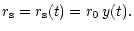
Here r0 is the starting radial density scale of the exploding material and the time dependence of the scale-length is found by determining y(t) from energy conservation.
By using a Gaussian profile, i.e.,
![$\exp[-(r/r_{\rm s})^2]$](/articles/aa/full/2001/04/aa10142/img9.gif) ,
to describe the density variation in the star, we find that a sphere of radius
,
to describe the density variation in the star, we find that a sphere of radius  contains about 43 percent of the mass of the star, we find that a sphere of radius
 contains about 95 percent of the mass. If we assume the progenitor star was in radiative equilibrium with
 ,
then from the Lane-Emden equation (see Chandrasekhar 1958) one gets a density profile for the star. If
,
then from the Lane-Emden equation (see Chandrasekhar 1958) one gets a density profile for the star. If  is the radius of this star, then by fitting the density to the Gaussian profile one finds that
 .
.
Some properties of the Gaussian model: the total mass M0 of the star and the gravitational energy per unit mass (GPE) are
 |
|
|
(3) |
where G is the gravitational constant. The gravitational force per unit volume is
![$\displaystyle F_{\rm g}=-[G\,\rho(r)/{r^2}]{\int_0^r}\,4\pi\rho(r')\,{r'}^2\,{\rm d}r'.$](/articles/aa/full/2001/04/aa10142/img16.gif) |
|
|
(4) |
The gravitational force is the one quantity that is not self-similar in this model, i.e.,
this force does not tend to maintain the Gaussian shape. However, it does do so at small r.
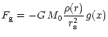
Equation (4) can be written as
 |
|
|
(5) |
where
![$\displaystyle g(x)=\left[{{\rm Erf}(x)-(2\,x/\sqrt{\pi})\,\exp(-x^2)}\right]$](/articles/aa/full/2001/04/aa10142/img18.gif) |
|
|
(6) |
and
 .
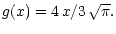
The function g(x) is linear for small x and can be approximated by a linear function out to x=1 after which there is substantial deviation. Now, the gravitational decelerating force is not the major force acting here, and it is only important in the very early stages of supernova expansion. We propose, therefore, to use the linear approximation for g(x) throughout, thus allowing it to be used in the similarity solution;
.
The function g(x) is linear for small x and can be approximated by a linear function out to x=1 after which there is substantial deviation. Now, the gravitational decelerating force is not the major force acting here, and it is only important in the very early stages of supernova expansion. We propose, therefore, to use the linear approximation for g(x) throughout, thus allowing it to be used in the similarity solution;
 |
|
|
(7) |
However, we use the exact expression for the gravitational potential energy, Eq. (3).
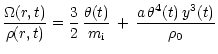
The internal energy (per unit mass) is taken to be
 |
|
|
(8) |
where a is the radiation constant, and the pressure p(r,t) is
![$\displaystyle p(r,t)={\rho(r,t)}\left[{\frac{\theta(t)}{m_{\rm i}}}+{\frac{a\,\theta^4\,(t)\,y^3(t)}{3\,\rho_{0}}}\right]$](/articles/aa/full/2001/04/aa10142/img22.gif) |
|
|
(9) |
where  is the central temperature of the star. Since the spatial dependence here (and below) has been removed, we will drop the (t) notation from
 .
.
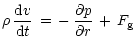
The functional forms from Eqs. (1) and (2) conserve mass. Substituting them into the radial momentum equation
 |
|
|
(10) |
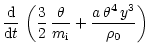
where  is given by Eqs. (5) and (7), we obtain an equation for the temperature (in energy units) in terms of the function y:
![$\displaystyle \theta\,+\,\frac{1}{3}\,\frac{a\,m_{\rm i}\,\theta^4\,{y^3}}{\rho...
...\,=\,\frac{m_{\rm i}r_{0}^2}{2}\,\left[y\,\ddot{y}+1/(\tau_{\rm g}^2\,y)\right]$](/articles/aa/full/2001/04/aa10142/img26.gif) |
|
|
(11) |
where the dots are time derivatives,  is the mass of an average ion
in the exploding material and
is the mass of an average ion
in the exploding material and
 .
.
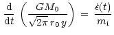
The problem is completed by specifying the energy sources driving the explosion and examining the energy conservation equation (per unit mass) which is given by
where we have taken the energy deposition to be proportional to the density. We choose the energy release rate per particle to be
 |
|
|
(13) |
where t1 and t2 are the mean times for the two energy-releasing processes.
 represents the energy supplied by either the nuclear explosion or gravitational collapse, and
 represents the longer term radioactive energy. We neglect surface radiation loss in Eq. (12); it is a small contribution to the overall energy balance. Equation (12) can be written
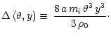
with
 |
|
|
(15) |
Equations (11) and (14) form a set of coupled ordinary differential equations which can be integrated numerically subject to the initial conditions: y(0)=1,  ,
and
,
and
 .
Note that Eq. (11), expressing momentum balance, determines the initial temperature
.
Note that Eq. (11), expressing momentum balance, determines the initial temperature
 of the progenitor star assuming
 .
.
Before proceeding to the integration of the ordinary differential equations, we introduce some normalized units. The mass and radius of the progenitor star in units of the sun's mass and radius is
 and
and
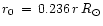
 (the parameter r should not be confused with the radial coordinate). The Gaussian "radius" for the progenitor having mass equivalent to that of the progenitor,
 .
The progenitor's central density
.
The progenitor's central density
 .
Having chosen a mass and radius for the progenitor, we calculate the GPE from Eq. (3) as
.
Having chosen a mass and radius for the progenitor, we calculate the GPE from Eq. (3) as
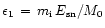
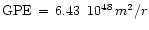 ergs. Further, we relate the supernova explosion energy to a multiple of the GPE as
 which is also related to
 .
We relate the later radioactive decay energy to the supernova explosion energy as
.
We relate the later radioactive decay energy to the supernova explosion energy as
 .
Finally, we take the decay time in terms of the
.
Finally, we take the decay time in terms of the
![$\element[][56]{Ni}$](/articles/aa/full/2001/04/aa10142/img52.gif) decay time,
decay time,
 s.
s.
Now, it is believed that the long-period energy release in supernovae comes from the radioactive decay of
followed by the decay of daughter
![$\element[][56]{Co}$](/articles/aa/full/2001/04/aa10142/img54.gif) .
The mean life of
is 8.8 days and the mean life of the daughter is 111 days. Because of the well-known gamma-ray transparency issue (see Arnett 1996), we do not expect the mean life of decay for the light curve to be a simple amalgamation of the Ni-Co decays, but rather somewhat shorter (see below).
.
The mean life of
is 8.8 days and the mean life of the daughter is 111 days. Because of the well-known gamma-ray transparency issue (see Arnett 1996), we do not expect the mean life of decay for the light curve to be a simple amalgamation of the Ni-Co decays, but rather somewhat shorter (see below).
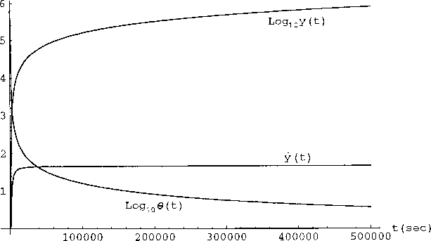
Returning now to the ordinary differential equations, Eqs. (11) and (14), and using the definitions above, we have made numerous numerical integrations of this system using Mathematica (1999) for stars typical in size and mass of type I supernovae.
 |
Figure 1:
A representative similarity model calculation of the normalized radius y(t), the normalized velocity
 ,
and the temperature ,
versus time. The parameters (see text for definitions) were: ,
and the temperature ,
versus time. The parameters (see text for definitions) were:
 |
| Open with DEXTER |
For example, Fig. 1 shows the results of one such integration for an
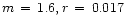 progenitor with
  .
The radius and velocity are obtained by multiplying y and
.
The radius and velocity are obtained by multiplying y and  by
by
 cm. The temperature
is in eV and to begin the integration a root finder is used to determine the starting
cm. The temperature
is in eV and to begin the integration a root finder is used to determine the starting
 eV required for momentum balance in Eq. (11). We note that the temperature determined from our momentum balance is in reasonable agreement with Chandrasekhar's polytropic temperature for the radiative-equilibrium, progenitor star.
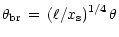
We now calculate the luminous power radiated using the fourth power of the surface temperature and the surface area which is proportional to y2. Our model gives a surface temperature in terms of the central temperature; however, it is not accurate because the actual surface temperature depends upon the star's internal structure, specifically the opacity of the star. Instead, we choose to use a relationship suggested by Zeldovich (1967) which expresses the surface brightness temperature of an optically thick radiating body of dimension  in terms of its central temperature
  :
:
 |
|
|
(16) |
where  is photon mean free path. Chandrasekhar (1958) gives the opacity
 and the mean free path goes as
 .
We take the dimension
.
We take the dimension
 with
with
 .
Finally, to keep the brightness temperature from becoming larger than the central temperature when the density becomes very low, we impose a limit by setting
.
Finally, to keep the brightness temperature from becoming larger than the central temperature when the density becomes very low, we impose a limit by setting
![$\displaystyle \theta_{\rm br}\,=\,\frac{(\ell/x_{\rm s})^{1/4}}{\left[1+(\ell/x_{\rm s})\right]^{1/4}}\,\theta\cdot$](/articles/aa/full/2001/04/aa10142/img70.gif) |
|
|
(17) |
Before we calculate the supernova's luminosity as a function of time, we model the so-called gamma-ray transparency issue (see Arnett 1996). Up to this point, the model permits all of the radioactive energy produced to be absorbed. However, when the debris density becomes sufficiently low, some of the gamma-ray energy escapes and doesn't contribute to driving the expansion. Therefore, we multiply the radioactive-decay, energy term
 in Eq. (13) by an absorption fraction given by
![$\displaystyle {A(t)}=\left[1-\exp{\left(-\kappa\,\int_0^{\infty}\,\rho\,{\rm d}r\right)}\right]$](/articles/aa/full/2001/04/aa10142/img72.gif) |
|
|
(18) |
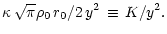
where  is an energy-averaged (gamma-ray) absorption coefficient. Using the model's Gaussian density profile the integral can be done, yielding
 |
|
|
(19) |
Hence,
![$\displaystyle {A(t)}=\left[1-\exp{\left(-K/y^2\right)}\right].$](/articles/aa/full/2001/04/aa10142/img75.gif) |
|
|
(20) |
In effect, this procedure modifies the time constant of the radioactive energy production in the expanding star, so that a fit of the model to the experimental data will yield an effective value of t2 that is smaller than the radioactive decay time constant.
This completes our similarity model for calculating the light curves from the supernovae. We now apply the model to recent data on type I supernovae from the Supernova Cosmology Project (1998) (SCP).
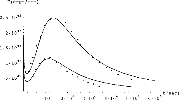
The SCP has recorded light curves from a number of type I supernova observations. We have chosen to examine the data which we refer to as the "orange" data set (the highest luminosity data set of the observations) and the "green" data set (the lowest luminosity data set). We "read" the data points from the orange and green sets from the SCP website with some associated errors not easily estimated. The apparent magnitudes MV, were converted to luminosity assuming a Hubble constant  kms-1/Mpc and
 .
The luminosity data do not, of course, have a zero time indication so there is some latitude in extracting the model parameters by adjusting the zero-time point. Also, the similarity model allows a choice of parameters that may be varied and a radiated power profile to be calculated. Therefore, a number of integrations were required to find the approximate values of the progenitor's mass and radius. These set the energy scale necessary to explode the star. After adjusting the mass and radius and adjusting the ratio of explosion energy to GPE, the ratio
.
The luminosity data do not, of course, have a zero time indication so there is some latitude in extracting the model parameters by adjusting the zero-time point. Also, the similarity model allows a choice of parameters that may be varied and a radiated power profile to be calculated. Therefore, a number of integrations were required to find the approximate values of the progenitor's mass and radius. These set the energy scale necessary to explode the star. After adjusting the mass and radius and adjusting the ratio of explosion energy to GPE, the ratio
 can be varied to get the approximate magnitude of the luminosity correct. There is some sensitivity to the choice of t1 as well, but values between 1000 and 2000 s seemed to give the best fits and are appropriate for stars of this size.
 |
Figure 2:
The SCP orange (higher power points) and green (lower power points) data sets along with the best fits from the similarity model (lines). The orange fitting parameters were:
 ,
and the green fitting parameters were: ,
and the green fitting parameters were:
 |
| Open with DEXTER |
Our best fits to the SCP orange and green data sets are shown in Fig. 2; the best fit parameters are shown in the figure caption. Notice that the green data seem to represent a supernova from a rather small progenitor actually somewhat under the Chandrasekhar limit. Also, average energy per ion
is about 10.5 MeV, and the ratio of explosion energy to the GPE for both cases is similar. We found that the parameter space allowing a "fairly good" fit was rather limited, both by requiring smaller stars and the choice of energy
for the later radioactive decay luminosity. Finally, the large number of digits in the initial temperature is a result of the fact that without sufficient precision at the start of the integration, the numerical noise makes the system unstable and usually fails.
The model-fitting integrations run quickly on a PC so that a large number of comparisons to the observed light curves can be performed without invoking more complex (and lengthy) programs.
The model described above results in a simple set of ordinary differential equations which are easily solved numerically. Each example can be integrated on a modest PC with, e.g., Mathematica, and plotted in less than a minute. This permits the possibility of carrying out a number of detailed parametric studies. Since our model effectively decouples the spatial and temporal variables, modifications to the model can be made easily as was done, for example, in the case of the gamma-ray transparency problem. The model has clear limitations and is not a substitute for full radiation-hydrodynamic codes. However, because it conserves mass, momentum, and energy, the dynamic results and scaling connection between parameters are expected to be fairly accurate. The price paid for the model's simplicity is the lack of detailed knowledge of energy transport and of temperature-dependent energy-producing reactions throughout the star.
We have limited our numerical studies to type I supernovae. We have found that to obtain physical solutions to the equations the mass of the progenitor star should be
 and that these small stars also need a small initial radius
 .
The energy
.
The energy
 must exceed the GPE in order for the expansion to proceed, and it must exceed that energy by about 20 percent or more to avoid initial instabilities in the early stages of expansion. Although this self-similar model is not a substitute for detailed three-dimensional hydrodynamic and radiation transport studies, we feel that it should be useful in providing a framework for setting up such calculations and for analyzing experimental data.
The model, with a few changes in the starting parameters, should also be suited to study type II supernovae light curves.
-
Arnett, D. 1996, Supernovae and Nucleosynthesis (Princeton University Press, Princeton, NJ), Chapter 13, Appendix D, 439
In the text
-
Blinnikov, S. I., & Popov, D. V. 1993, A&A, 274, 775
NASA ADS
-
Chandrasekhar, S. 1958, An Introduction to the Study of Stellar Structure (Dover Publications, Inc., New York, NY), 87, 293
In the text
-
Mayer, F., & Tanner, D. 1981, Annals New York Acad. Sci., 373, 68
In the text
-
Pinto, P. A., &
Eastman, R. G. 2000, ApJ, 530, 744
NASA ADS
-
Mathematica-V4 1999, Wolfram Research, Inc., Champaign, IL 61820
In the text
-
Sedov, L. 1959, Similarity and Dimensional Methods in Mechanics (Academic Press, New York), Chapter 4
In the text
-
Supernova Cosmology Project 1998, Lawrence Berkeley Laboratory,
The data presented here was read from the SCP poster from the January meeting of the American Astronomical Society on the website: In the text
http://supernova.lbl.gov
-
Zeldovich, Ya., & Raizer, Yu. 1967, Physics of Shock Waves and High-Temperature Hydrodynamic Phenomena, vol. II. (Academic Press, New York), Chapter XII, 165
In the text
Copyright ESO 2001

![$\displaystyle \dot{\theta}\,\left[1+\Delta\,(\theta,y)\right]\,$](/articles/aa/full/2001/04/aa10142/img35.gif)
![$\displaystyle \frac{2}{3}\,\dot{\epsilon}\,-\,\frac{\dot{y}\,\theta}{y}\,\left[2+\Delta\,(\theta,y)\,\right]$](/articles/aa/full/2001/04/aa10142/img36.gif)