2 Observations and results

Eight quasars have been observed with ISO in revolution 169-781 (1996 March - 1998 January). Optical and near-infrared imaging observations have followed within 24 months (mostly within 17 months).

2.1 The sample

 

 

Table 1: Quasars' sample

Object	RA (J2000) Dec.		z	MBa	Radiob	Rev (UT)c	Other name and Notes
PC 1548+4637	15:50:07.6	+46:28:55	3.544	-27.0	Quiet	169 (960504)
PC 1640+4628	16:42:05.1	+46:22:27	3.700	-26.8	Quiet	185 (960520)
H 0055-2659	00:57:58.1	-26:43:14	3.662	-29.2	Optical	380 (961130)
UM 669	01:05:16.8	-18:46:42	3.037	-28.4	Optical	415 (970104)	Q 0102-190
B 1422+231	14:24:38.1	+22:56:01	3.62	-29.8d	Loud	424 (970113)	Lensed quasar
PG 1630+377	16:32:01.1	+37:37:49	1.478	-28.2	Quiet	424 (970113)	Also observed on rev. 778 (980101)
PG 1715+535	17:16:35.4	+53:28:15	1.940	-28.5	Quiet	712 (971027)
UM 678	02:51:40.4	-22:00:27	3.205	-29.4	Optical	781 (980104)	Q 0249-222

^a The absolute B magnitude for H₀ = 75 km s^-1 Mpc^-1 with q₀ = 0.0.

^b Radio property; Quiet = radio quiet, Loud = radio loud, and Optical = optically selected.

^c UT is given in the yymmdd format where yy = year, mm = month, and dd = day.

^d $M_{B}\sim -26$ after demagnification (Kormann et al. 1994).

Table 1 lists the sample of the eight quasars in the sequence of ISO revolutions for execution. The sample consists of luminous quasars with M_B < -28 except PC 1548+4637 and PC 1640+4628; these two quasars which were observed at the beginning of this work, turned out to be too faint to be detected in the far-infrared, and thus the sample selection criterion was changed to include very luminous quasars in low far-infrared background of infrared cirrus emission. Figure 1 presents the eight quasars (large filled diamonds) on the z - M_B plane together with those (small filled circles) in the sample by Elvis et al. (1994) and those (faint gray points) complied by Véron-Cetty & Véron (1998). All the sample quasars are radio-quiet or optically selected except B 1422+231 which is a core-dominant flat-spectrum radio source.

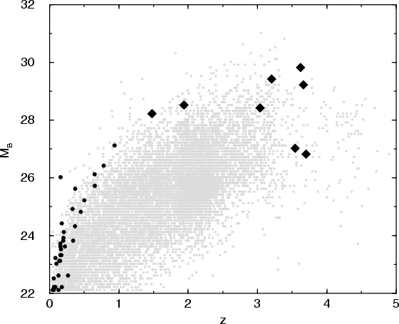Figure 1: Sample quasars (large filled diamonds) compared with other samples of quasars on the z - MB plane. Small filled circles show quasars studied by Elvis et al. (1994). Quasars cataloged by Véron-Cetty & Véron (1998) were plotted by dots, which appears as a gray background on this plane

2.2 Mid-infrared observations with ISOCAM

The mid-infrared observations were performed with ISOCAM (Cesarsky et al. 1996). Three broad band filters, namely, LW2 (reference wavelength 6.7 $\mu$m), LW3 (14.3 $\mu$m), and LW10 (12.0 $\mu$m) were used. All the quasars were observed in LW2 with additional measurements in LW3 or LW10. To detect faint sources against the intense background dominated by zodiacal light, the AOT (Astronomical Observation Template) CAM01 which is the microscan raster mapping mode was used to achieve accurate flat-fielding (e.g., Taniguchi et al. 1997; Altieri et al. 1999). Table 2 lists the details of CAM01 parameters as well as the characteristics of the broad band filters.

The standard ISOCAM reduction software CIA 3.0 was used to produce ISOCAM images from ERD (Edited Raw Data). This process includes dark subtraction, deglitching, correction for the transient behavior of ISOCAM pixel signals, and flat fielding (Delaney 1998). The inversion transient correction model of Starck et al. (1999) was applied. The factor of the correction for the transient behavior is 0.58-0.77 in LW2, 0.79-1.0 in LW10, and 0.87 in LW10. 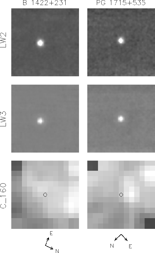Figure 2 shows LW2 and LW3 maps for the two brightest quasars B 1422+231 and PG 1715+535. All the quasars were clearly detected at the expected positions. Aperture photometry was performed using IDL. Two apertures centered on the object were used; the small one has a diameter of $2d_{\rm airy}$, two times the Airy diameter as given in Table 2 and the other has a diameter of $4d_{\rm airy}$. The photometry was corrected for loss of flux in the PSF (Point Spread Function) wings by computing the PSF based on the model having a two mirror f/15 telescope with radii for the primary and secondary mirror of 30 and 10 cm, respectively (Müller 1999). The factor of the PSF correction is 0.75-0.90 (i.e., loss of flux is 0.1-0.25), depending on the raster step and the pixel field of view.

 

 

 

Table 2: Filters and settings for raster mapping

Filtera	LW2	LW3	LW10	C_90	C_160
$\lambda_{\rm ref}$	6.7 $\mu$m	14.3 $\mu$m	12.0 $\mu$m	90 $\mu$m	170 $\mu$m
$\Delta\lambda$	3.5 $\mu$m	6.0 $\mu$m	7.0 $\mu$m	51 $\mu$m	89 $\mu$m
Airy diameterb	5.6 $^{\prime \prime }$	12.0 $^{\prime \prime }$	10.1 $^{\prime \prime }$	76 $^{\prime \prime }$	143 $^{\prime \prime }$
	Raster points M $\times$ N, Raster step, Exposure time per raster pointc, Pixel field of view
QSO field	LW2	LW3	LW10	C_90	C_160
PC 1548+4637	$5 \times 2$, 6 $^{\prime \prime }$, 60 s, 6 $^{\prime \prime }$	...	$4 \times 1$, 6 $^{\prime \prime }$, 25 s, 6 $^{\prime \prime }$	$4 \times 4$, 44 $^{\prime \prime }$, 64 s, 44 $^{\prime \prime }$	$3 \times 3$, 90 $^{\prime \prime }$, 64 s, 89 $^{\prime \prime }$
PC 1640+4628	$5 \times 2$, 6 $^{\prime \prime }$, 60 s, 6 $^{\prime \prime }$	...	$4 \times 1$, 6 $^{\prime \prime }$, 25 s, 6 $^{\prime \prime }$	$4 \times 4$, 44 $^{\prime \prime }$, 64 s, 44 $^{\prime \prime }$	$3 \times 3$, 90 $^{\prime \prime }$, 64 s, 89 $^{\prime \prime }$
H 0055-2659	$5 \times 2$, 6 $^{\prime \prime }$, 60 s, 6 $^{\prime \prime }$	...	...	$5 \times 3$, 44 $^{\prime \prime }$, 69 s, 44 $^{\prime \prime }$	$4 \times 2$, 90 $^{\prime \prime }$, 73 s, 89 $^{\prime \prime }$
UM 669	$6 \times 6$, 7 $^{\prime \prime }$, 90 s, 3 $^{\prime \prime }$	...	...	...	$10 \times 10$, 46 $^{\prime \prime }$, 16 s, 89 $^{\prime \prime }$
B 1422+231	$4 \times 4$, 7 $^{\prime \prime }$, 90 s, 3 $^{\prime \prime }$	$4 \times 4$, 7 $^{\prime \prime }$, 90 s, 3 $^{\prime \prime }$	...	...	$10 \times 10$, 46 $^{\prime \prime }$, 16 s, 89 $^{\prime \prime }$
PG 1630+377d	$4 \times 4$, 7 $^{\prime \prime }$, 38 s, 3 $^{\prime \prime }$	$4 \times 4$, 7 $^{\prime \prime }$, 38 s, 3 $^{\prime \prime }$	...	...	$10 \times 10$, 46 $^{\prime \prime }$, 16 s, 89 $^{\prime \prime }$
PG 1715+535	$4 \times 4$, 7 $^{\prime \prime }$, 38 s, 3 $^{\prime \prime }$	$4 \times 4$, 7 $^{\prime \prime }$, 38 s, 3 $^{\prime \prime }$	...	...	$10 \times 10$, 46 $^{\prime \prime }$, 16 s, 89 $^{\prime \prime }$
UM 678	$4 \times 4$, 7 $^{\prime \prime }$, 90 s, 3 $^{\prime \prime }$	$4 \times 4$, 7 $^{\prime \prime }$, 90 s, 3 $^{\prime \prime }$	...	...	$6 \times 5$, 92 $^{\prime \prime }$, 64 s, 89 $^{\prime \prime }$

^a Cited from $ISO\ Handbook\ Volume\ III\ (CAM)$ (Siebenmorgen et al. 1999) and $Volume\ V\ (PHT)$.

^b The aperture photometry was performed by using the apertures with a diameter of $2\times d_{\rm airy}$ for ISOCAM and of $d_{\rm airy}$ for ISOPHOT. The diameter of the Airy disk $d_{\rm airy}$ is $2.44(\lambda/60~{\rm cm})$ in radian or $0.84\lambda~(\mu$m) in arcsec. Note that the FWHM of the Airy disk is $0.422 \times d_{\rm airy}$.

^c ISOCAM exposure time per raster point is given as $T_{\rm int}\times N_{\exp}$ where $T_{\rm int}$ is an integration time of a single exposure and $N_{\exp}$ is the number of exposures. $T_{\rm int}= 5$ s was used for all LW2 and LW3 observations except for PG 1630+377 and PG 1715+535 for which $T_{\rm int}=2$ s was used. $T_{\rm int}=2$ s was used for LW10 observations.

^d The second observation was executed on revolution 778 in C_160 with a parameter set of ( $6 \times 6$, 92 $^{\prime \prime }$, 64 s, 89 $^{\prime \prime }$).

 

 

Table 3: ISO mid/far-infrared flux density and UV to IR luminosity. This table is also available in electronic form at the CDS
via anonymous ftp to cdsarc.u-strasbg.fr (130.79.128.5)
or via http://cdsweb.u-strasbg.fr/cgi-bin/qcat?J/A+A/365/409

	ISOCAM (mJy)				ISOPHOT (mJy)			Luminosity $~(10^{13}L_{\odot})^a$
Object	LW2	LW3	LW10		C_90	C_160		$L_{\rm UVO}$	$L_{\rm ir}$	$L_{1.25~\mu{\rm m}}$
PC 1548+4637	$0.16\pm0.04$	...	$0.67\pm0.17$		$8.2\pm28$	$32\pm80$		11	<130	1.7
PC 1640+4628	$0.15\pm0.04$	...	$0.29\pm0.11$		$-8.3\pm20$	$83\pm121$		8.1	<240	1.8
H 0055-2659	$0.29\pm0.06$	...	...		$16\pm19$	$-2.7\pm60$		24	<160	3.3
UM 669	$0.50\pm0.01$	...	...		...	$-9.9\pm18$		27	<39	3.5
B 1422+231	$5.8\pm0.06$	$15.1\pm0.07$	...		...	$83\pm56$		410	<320	64
PG 1630+377	$4.3\pm0.04$	$7.3\pm0.07$	...		...	$5.6\pm14$b		28	<16	4.3
PG 1715+535	$4.7\pm0.06$	$10.3\pm0.06$	...		...	$-13\pm16$		81	<26	9.4
UM 678	$0.73\pm0.01$	$1.9\pm0.03$	...		...	$-15\pm58$		30	<116	5.9

^a The UVO ($0.1~\mu$m to $1~\mu$m) luminosity $L_{\rm UVO}$ = $4\pi D_{\rm L}^{2} \times 2.3\int_{14.5}^{15.5}\nu f_\nu {\rm d}\log_{10}\nu$, the IR ($1.5~\mu$m to $100~\mu$m) luminosity $L_{\rm ir}$ = $4\pi D_{\rm L}^{2} \times 2.3 \int_{12.5}^{14.3}\nu f_\nu {\rm d}\log_{10}\nu$, and the $1.25~\mu$m luminosity $L_{1.25~\mu{\rm m}}$ = $4\pi D_{\rm L}^{2}\nu f_\nu$, where $D_{\rm L}$ and $f_{\nu}$ denote the luminosity distance and observed flux density, respectively. Where no observations exist such as $1~\mu$m flux densities, interpolated flux densities were used. $L_{\rm UVO}$ is based on the optical and near-infrared flux densities given in Table 4.

^b $f_\nu(170~\mu{\rm m}) = 89\pm78$ mJy was obtained in the second observation.

Figure 2: ISOCAM LW2 (6.7 $\mu$m) and LW3 (14.3 $\mu$m) and ISOPHOT C_160 (170 $\mu$m) maps are shown on the top, middle, and bottom panels, respectively. B 1422+231 shown on the left was observed on revolution 424 and PG 1715+535 on revolution 712. The ISOCAM and ISOPHOT maps are 90 $^{\prime \prime }$ and 598 $^{\prime \prime }$(10$^\prime$), respectively, with North and East as indicated by the arrows. Quasars should be at the center of the gray circles

The results after these corrections are given in Table 3 with statistical errors. The errors in the absolute photometric calibration are not included in Table 3; these errors are estimated to be 15% (Siebenmorgen et al. 1999).

2.3 Far-infrared observations with ISOPHOT

The far-infrared observations were made with ISOPHOT (Lemke et al. 1996). All the quasars were observed in the broad C_160 (170 $\mu$m) band with additional measurement in C_90 (90 $\mu$m). ISO far-infrared surveys (Kawara et al. 1998; Puget et al. 1999) clearly indicate that the sky seen in the far-infrared has a clumpy structure which is made up of IR cirrus and extragalactic sources. This structure rotates with time relative to the ISO coordinate system due to the field rotation, increasing the probability of fault detection if the chopping mode is used. We thus selected the PHT22 staring raster map mode to make small maps around the quasar. Table 2 presents the characteristics of the photometric filters and the details of observational parameters for raster mapping.

ISOPHOT images were produced by using the standard ISOPHOT reduction software PIA V7.3 and V8.1 (Gabriel et al. 1997), starting at the edited raw data (ERD) created via the off-line processing version 7.0. The AOT/Batch processing mode of PIA is used with the default parameters to reduce ERD to the Astronomical Analysis Processing (AAP) level. This standard reduction includes linearization and deglitching of integration ramps on the ERD level, signal deglitching and drift recognition on the SRD (Signal per Ramp Data) level, reset interval normalization, signal deglitching, dark current subtraction, signal linearization, and vignetting correction on the SCP (Signal per Chopper Plateau data) level. The responsivity calibration was made on the SPD (Standard Processed Data) level by using the second measurement of the internal Fine Calibration Source 1 (FCS1) which is calibrated against celestial standards. The correction for the transient behavior of the detectors was applied to point sources (quasars) on this level. Images were produced on the AAP (Astronomical Analysis Processing) in the mapping mode with median brightness values.

The correction for drift in the responsivity is not important to our observations, and so this correction was not made. To check the importance of the drift, the MEDIAN filter technique was applied to the results from AAP (hereafter called AAP map). Applying this technique to large AAP maps in the Lockman hole, Kawara et al. (1998) show that this is a powerful tool to correct for drift in the detector responsivity. However, unlike large AAP maps in the Lockman hole, the MEDIAN filter technique does not improve our AAP maps. This is attributed to the size of our AAP maps; the observing time of these small maps is shorter than the timescale of drift in the detector responsivity, and so impact by the drift is small. In fact, every detector pixel of the C100 and C200 detector arrays has been checked for signal, and neither spike noise nor drift in the responsivity was found. Maps with all the detector pixels always give better results than those obtained by masking some of the detector pixels. In addition, it was confirmed that there were no significant differences between two AAP maps produced by two different algorithms on the AAP level, namely, the full coverage and distance weighting algorithms. Figure 2 shows AAP maps of C_160 for the brightest quasars B 1422+231 and PG 1715+535.

Aperture photometry was then performed using IRAF and Skyview in the manner similar to ISOCAM. The original pixel sizes of AAP maps are equal to the raster steps. Because these are too large to center the aperture on the quasar with sufficient accuracy, AAP maps were rebinned in such a way that each original pixel is converted into $10 \times 10$ sub-pixels. Two apertures centered on the object were used; the small one has a diameter of $d_{\rm airy}$, the Airy diameter as given in Table 2, and the other has a diameter of $2d_{\rm airy}$. The photometry was corrected for loss of flux in the PSF (Point Spread Function) wings by computing the same PSF model as used for ISOCAM. The factor of the PSF correction is 0.63 except for PC 1548+4632 and PC 1640+4628. These two quasars were centered between four pixels in such a way that quasars illuminate the four pixels equally. Consequently the loss of flux measured with the two apertures is large, and the factor of the PSF correction is 0.27 for C_90 and 0.23 for C_160.

The results after these corrections are given in Table 3 with statistical errors. The errors in the absolute photometric calibration are not included in Table 3; these errors are estimated to be 30% (Klaas et al. 2000). It is noted that PG 1630+377 was observed twice at $170~\mu$m to check variability.

 

 

Table 4: Optical to near-infrared magnitudes. This table is also available in electronic form at the CDS via anonymous ftp to cdsarc.u-strasbg.fr (130.79.128.5) or via http://cdsweb.u-strasbg.fr/cgi-bin/qcat?J/A+A/365/409

This work
Object	V	R	I	J	H	$K^{\prime a}$	UTb	Obs.c
PC 1640+4628	$20.13\pm0.12$	$19.38\pm0.16$	$18.80\pm0.15$	...	...	...	970828	Kiso
PC 1640+4628	...	...	...	...	$17.8\pm 0.2$	...	980606	OAO
H 0055-2659	$18.17\pm0.02$	$17.79\pm0.02$	$17.69\pm0.03$	...	...	...	971018	CTIO
UM 669	$17.65\pm0.01$	$17.47\pm0.01$	$17.23\pm0.02$	...	...	...	971018	CTIO
PG 1630+377	$16.13\pm0.01$	$15.76\pm0.16$	$15.51\pm0.15$	...	...	...	970824	Kiso
PG 1630+377	...	...	...	$14.92\pm0.03$	$14.38\pm0.01$	$14.12\pm0.04$	980603	OAO
UM 678	$17.63\pm0.02$	$17.62\pm0.02$	$17.30\pm0.03$	...	...	...	971018	CTIO
Data from others
Objectd	$u^\prime$	$g^\prime$	$r^\prime$	$i^\prime$	$z^\prime$	UT		Obs.e
PG 1715+535	16.53	15.89	15.47	15.25	15.24	July 1995		R
PG 1630+377	16.27	16.13	15.94	15.83	15.70	July 1995		R
B 1422+231	...	16.33	15.18	15.07	...	July 1995		R
PC 1548+4637	...	...	19.27f	...	...	April 1987		S

^a The $K^\prime$ bandpass filter ( $2.15\pm0.15~\mu$m) is slightly narrower and bluer than the standard K filter ( $2.20\pm0.20~\mu$m).

^b Universal time when observed in the yymmdd format.

^c At the Kiso Observatory, the 2048² CCD with 1.5 $^{\prime \prime }$ per pixel was used on the 105 cm Schmidt telescope.
At CTIO, the 2048² CCD with 0.4 $^{\prime \prime }$ per pixel was used on the 90 cm telescope.
At OAO (Okayama Astrophysical Observatory), the infrared imager spectrometer which has a HgCdTe 256² detector array with 0.97 $^{\prime \prime }$ per pixel was used on the 188 cm telescope.

^d All but PG 1548+4637 were observed within 27 months before the ISO observations.

^e R = Richards et al. (1997); S = Schneider et al. (1994).

^f The r₄ bandpass was used.

2.4 Optical and near-infrared data from ground-based observations

Optical images were taken on the 0.9 m telescopes at CTIO and the Schmidt 1.05 m telescope at Kiso Observatory. Near-infrared imaging was made in the standard dithering mode on the 1.88 m telescope at the Okayama Astrophysical Observatory, NAOJ. SExtractor (Bertin & Arnouts 1996) was applied to the optical and near-infrared images to perform photometry. Flux calibration was made using the standards given by Landolt (1992) in the optical and the UKIRT faint standards (Casali et al. 1992) in the near-infrared. A typical photometric error is 0.05 mag.

Table 4 presents magnitudes of the quasars together with statistical errors. As shown in the table, all the ground-based observations were performed within 24 months (mostly 17 months) from the ISO observations so as to reduce the chance of having flux variations between ISO and ground-based observations. Table 4 also supplements optical magnitudes taken by Richards et al. (1997) and Schneider et al. (1994). All the supplementary quasars but PG 1548+4637 were observed within 27 months before the ISO observations.