![[*]](/icons/foot_motif.gif)
A&A 365, 598-611 (2001)
DOI: 10.1051/0004-6361:20000052
P. Hennebelle1 - M. Pérault1 - D. Teyssier1 - S. Ganesh2
Send offprint request: M. Pérault,
1 - Laboratoire de Radioastronomie Millimétrique, UMR 8540
du CNRS, École Normale Supérieure et Observatoire de Paris,
24 rue Lhomond, 75231 Paris Cedex 05, France
2 - Physical Research Laboratory, Navarangpura, Ahmedabad 380009, India
Received 28 July 2000 / Accepted 24 October 2000
Abstract
The ISO galactic survey provides images of the inner disk in two broad
filters (around 7 and 15  m) over some 15 square degrees, away
from the brightest star forming regions.
A multiresolution analysis of the images leads to a catalogue of infrared dark
clouds, most of which are condensed cores of large molecular clouds,
several kpc away from the Sun, seen in absorption in front of the
diffuse galactic emission. The longitude distributions of the
background emission and of the dark clouds correlate with known
tracers of young population components.
We analyse the morphology of the dark clouds and the intensity
fluctuations within the cloud boundaries at the two wavelengths.
The 7 to 15 m contrast ratio is
m) over some 15 square degrees, away
from the brightest star forming regions.
A multiresolution analysis of the images leads to a catalogue of infrared dark
clouds, most of which are condensed cores of large molecular clouds,
several kpc away from the Sun, seen in absorption in front of the
diffuse galactic emission. The longitude distributions of the
background emission and of the dark clouds correlate with known
tracers of young population components.
We analyse the morphology of the dark clouds and the intensity
fluctuations within the cloud boundaries at the two wavelengths.
The 7 to 15 m contrast ratio is
 for the clouds
located away from the Galactic Centre (
for the clouds
located away from the Galactic Centre (
 )
and
)
and
 for the clouds closest to
the Galactic Centre (
for the clouds closest to
the Galactic Centre (
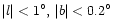 ).
Using a simple absorption model, we derive a 7 to 15 m opacity ratio
equal to
).
Using a simple absorption model, we derive a 7 to 15 m opacity ratio
equal to
 for the clouds located away from the Galactic Centre
and estimate the opacity,
for the clouds located away from the Galactic Centre
and estimate the opacity,  ,
of a few objects at 15 m
in the range 1 to 4.
Several explanations for the variation of the contrast ratio,
including absorption along the line of sight and local
variations of the extinction curve are discussed.
,
of a few objects at 15 m
in the range 1 to 4.
Several explanations for the variation of the contrast ratio,
including absorption along the line of sight and local
variations of the extinction curve are discussed.
Key words: ISM: clouds, dust, structure - Galaxy: structure - infrared: general
Author for correspondance: This email address is being protected from spambots. You need JavaScript enabled to view it.
m. Following studies established that
the mid-infrared emission from the solar neighbourhood was dominated
by diffuse emission, namely re-radiated stellar light from solid
particles and aggregates (Boulanger & Pérault 1988). These results
were extended to galactic scale (Pérault 1987). The mid- to far-IR
colour modulations due to the respective contributions of equilibrium
and non-equilibrium thermal emission by dust were emphasized, and
evidence was given of interstellar extinction in the most central
regions at 12 m, a result not inconsistent with standard
extinction curves and estimated line-of-sight column densities. The
quality of the mid-infrared images, limited by the accuracy of
zodiacal emission modelling, unfortunately restricted all published
IRAS galactic studies (e.g. Sodroski et al. 1989, 1994; Bloemen et al. 1990) to
the 60 and 100 m bands. Fortunately enough, COBE/DIRBE succeeded
(under other things) in producing an accurate zodiacal emission model
(Kelsall et al. 1998), and sensitive galactic emission
measurements at low angular resolution, which however, as far as we
know, have not been much exploited at mid-infrared wavelengths yet.
Median resolution spectroscopy on the other hand, especially from the
ISO short wavelength spectrometer, has provided a spectacular new
insight into physico-chemical properties of dust and gas, at least
close to bright enough sources.
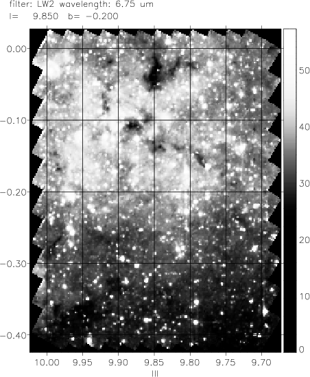 |
Figure 1:
9.85-0.20 field of the ISOGAL survey at 7 m.
The intensity scale is in
MJy sr-1. Positions are in galactic coordinates |
| Open with DEXTER | |
It turns out though that the mid-infrared wavelength range has not
been exhausted, and should still provide distinguished contributions
to studies of galactic diffuse components (large scale distribution
and properties of interstellar phases, disentanglement of stellar
distributions from absorption biases), as well as to studies of
stellar formation at galactic scale (detection of young stellar
populations throughout the disk, heating budget for the interstellar
components). As a matter of fact, the contents of giant molecular
clouds, for instance the gas fraction and temperature as a
function of density, the density and pressure gradients in the
condensation fronts at various spatial scales, and even worse,
the links of their internal structure to their
kinematics and dynamics, are still poorly documented.
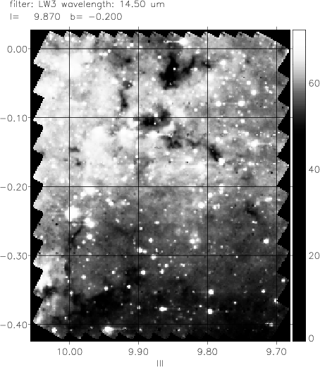 |
Figure 2:
Same field as Fig. 1 at 15 m |
| Open with DEXTER | |
The study of opaque condensed structures in a reasonably transparent
environment is a long-used approach of interstellar structures
(Barnard 1919; Bok 1947; Chandrasekhar & Münch 1952; Lynds 1962, ...).
ISO opened a similar opportunity in the
mid-infrared on galactic scales, with sub-parsec resolution (Pérault
et al. 1996) and detected many dark clouds in the inner
Galaxy. Shortly later the Mid-course space experiment's (MSX) infrared
imager surveyed the entire Galaxy, with a somewhat lower sensitivity
and angular resolution than the ISO camera, and detected some 2000
infrared dark clouds
mostly located between
 and
and
 which Egan et al. (1998) consider a new population
of cold dense isolated clouds.
Using H2CO observations, Carey et al. (1998)
inferred column
densities between 1023 and 1025 cm-2 and
densities around 105 cm-3.
which Egan et al. (1998) consider a new population
of cold dense isolated clouds.
Using H2CO observations, Carey et al. (1998)
inferred column
densities between 1023 and 1025 cm-2 and
densities around 105 cm-3.
The present paper reports
the first outcome of a systematic search of deep absorption features
in the 7 and 15 m images of the ISO galactic (scarse) survey
(ISOGAL: Omont et al. 1999).
A companion paper (Teyssier et al. 2001) will present
spectroscopic follow-up observations conducted at
the IRAM 30-m telescope on several dark objects.
It includes intensive observations of millimeter lines
of 13CO, C18O, HCN, HNC, HCO+, CH3C2H,
HC3N, and 1 mm continuum emission.
A subsequent study will focus on
a systematic correlation between the infrared dark clouds
and the stellar deficit in DENIS (near infrared) counts.
Section 2 briefly introduces the data and comments on
the variations of the galactic mid-infrared background
with longitude at 7 and 15 m.
In Sect. 3 we describe the systematic extraction
of the dark features with the help of a
multiscale analysis of the ISOGAL images.
The objects detected at 2 wavelengths are cross-identified,
and their morphology and distribution are then studied.
The intensity fluctuations in the dark objects are statistically
analysed in Sect. 4 and the mean 7 to 15 m opacity ratio is estimated.
A few individual clouds are further examined in Sect. 5, leading to
direct estimates of the optical depths.
The study of the clouds located near the
Galactic Centre and observed with narrower filters is
presented in Sect. 6. We then conclude in Sect. 7.
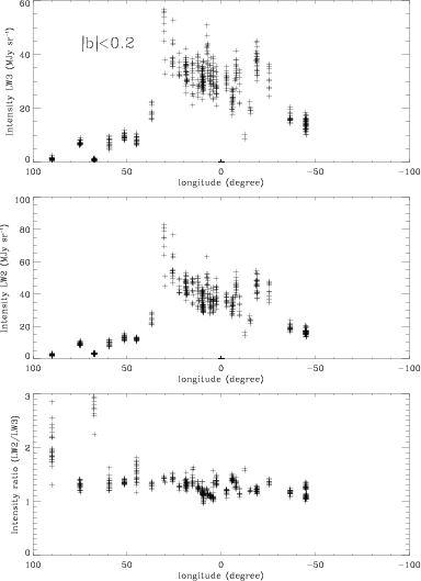 |
Figure 3:
Median intensity evaluated in square boxes of a
 area as a function of longitude for
 .
Intensities in LW2 and LW3
and their ratio are displayed .
Intensities in LW2 and LW3
and their ratio are displayed |
| Open with DEXTER | |
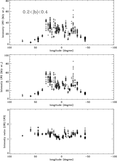 |
Figure 4:
Same as Fig. 3
for
|
| Open with DEXTER | |
Three different filters, LW2 (5-8.5), LW6 (7-8.5), and LW5 (6.5-7)
were used at
 and two filters
LW3 (12-18) and LW9 (14-16) around
and two filters
LW3 (12-18) and LW9 (14-16) around
 m.
The ISOGAL survey covers about 18
square degrees mainly in the inner Milky-Way around 7 and
m.
The distribution is as follows:
m.
The ISOGAL survey covers about 18
square degrees mainly in the inner Milky-Way around 7 and
m.
The distribution is as follows:
 )
has been observed with
the LW2 and LW3 filters (8.5 square degrees);
)
has been observed with
the LW2 and LW3 filters (8.5 square degrees);
 )
has been observed with
the LW2 and LW3 filters (3.5 square degrees);
)
has been observed with
the LW2 and LW3 filters (3.5 square degrees);
 )
has been observed with
the LW6 and LW9 filters (2.5 square degrees);
)
has been observed with
the LW6 and LW9 filters (2.5 square degrees);
 to be better than 1 MJy sr-1.
Figures 1 and 2
are two ISOGAL images of the same field at 7 m (LW2)
and 15 m (LW3).
Both prominent emission and
absorption features can be seen, as presented in earlier
ISOGAL papers (e.g. Pérault et al. 1996), bringing
deep insight into the structure of the interstellar medium,
throughout the Galactic Plane. Several dark features can be seen.
One of them ((
 ,
,
 ),
DF+9.85-0.05) is studied in detail (Sect. 5).
),
DF+9.85-0.05) is studied in detail (Sect. 5).
Figures 3 and 4 show
the median filtered intensity (in MJy sr-1)
of several lines of sight at low latitude
(
)
and
higher latitude (
)
respectively, as a function of longitude in the LW2 and LW3
filters. The intensity ratio is also shown.
The median is computed in square boxes of a
area. The intensities vary in a similar way as the IRAS sky
brightness, away from bright star forming regions.
The ratio between the two bands is strikingly
uniform:
 for all directions of not too low brightness
(where the uncertainty dominates).
for all directions of not too low brightness
(where the uncertainty dominates).
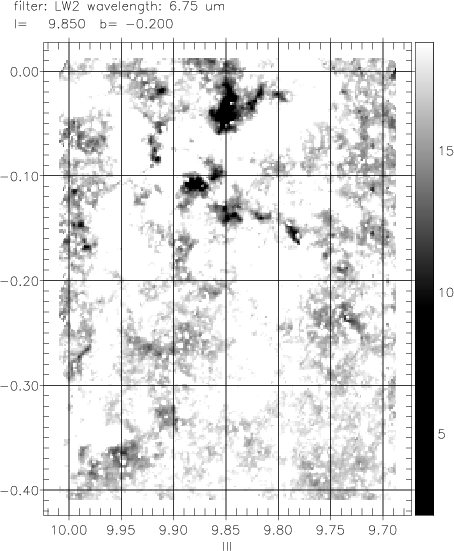 |
Figure 5:
7
LW2 image of the 9.85-0.20 field after
clipping of all positive structures |
| Open with DEXTER | |
In this section, we present a systematic detection of the dark objects seen in the ISOGAL images and statistically study some of their properties.
 )
in the background, at
the scale of an individual image (
)
in the background, at
the scale of an individual image (
 degree). Point sources or
extended sources add up to this contrasted background and to the
inherent complexity of these structures, preventing
simple algorithms from properly extracting the dark structures.
Although sophisticated multiscale analysis tools are
appropriate for complex extraction, they are not designed for
images with both positive and negative structures.
The following strategy was thus adopted:
degree). Point sources or
extended sources add up to this contrasted background and to the
inherent complexity of these structures, preventing
simple algorithms from properly extracting the dark structures.
Although sophisticated multiscale analysis tools are
appropriate for complex extraction, they are not designed for
images with both positive and negative structures.
The following strategy was thus adopted:
 0.5 square arcmin);
m lists.
0.5 square arcmin);
m lists.
 );
);
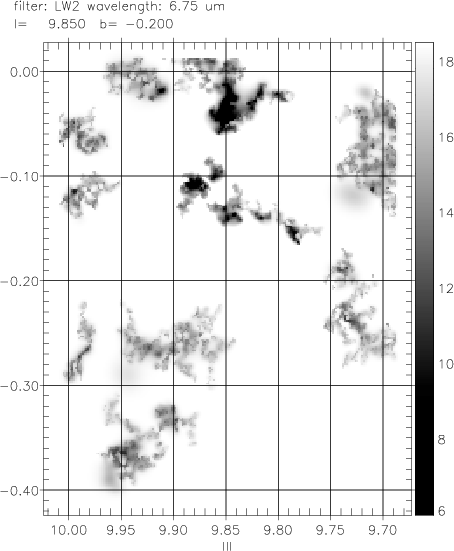 |
Figure 6: Reconstructed LW2 image of the 9.85-0.20 field using MVM |
| Open with DEXTER | |
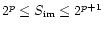 ,
where
,
where
 is the size
of the image), the reconstruction is limited to
scales between 2 and p-1.
Most of the reconstructed objects correspond to
diffuse patches of moderate absorption or to emission minima and are not relevant
for the present study. We thus only keep the objects for which
the contrast (ratio of the intensity deficit to the background intensity), C,
reaches at least 15% at one position of the object.
The resulting lists at 7 and 15 m are then cross-identified on
the basis of spatial coïncidence.
is the size
of the image), the reconstruction is limited to
scales between 2 and p-1.
Most of the reconstructed objects correspond to
diffuse patches of moderate absorption or to emission minima and are not relevant
for the present study. We thus only keep the objects for which
the contrast (ratio of the intensity deficit to the background intensity), C,
reaches at least 15% at one position of the object.
The resulting lists at 7 and 15 m are then cross-identified on
the basis of spatial coïncidence.
Figure 5 shows the result of the emission clipping
in the 9.85-0.20 field at 7 m.
Diffuse and more compact structures, partly connected, are present. The reconstructed
image obtained after performing all steps of MVM and applying
the minimal contrast criterion, is displayed in
Fig. 6.
All significant structures, mostly in the upper part of the map (above
 ), have been properly reconstructed.
The isolated diffuse structures
have been eliminated by the minimal contrast criterion whereas the
diffuse parts spatially connected to the denser ones remain.
Small structures at scale 1, like the feature located at
), have been properly reconstructed.
The isolated diffuse structures
have been eliminated by the minimal contrast criterion whereas the
diffuse parts spatially connected to the denser ones remain.
Small structures at scale 1, like the feature located at
 and
and
 ,
have not been reconstructed either.
One of the limitations of MVM is that, using square wavelets, narrow
filaments are detected as lines of scale 1 elements, and thus fall off
the catalogue.
,
have not been reconstructed either.
One of the limitations of MVM is that, using square wavelets, narrow
filaments are detected as lines of scale 1 elements, and thus fall off
the catalogue.
The clipped and reconstructed LW3 images (Fig. 2)
are displayed in Figs. 7 and 8.
Similar results to LW2 are obtained for the denser parts
(but for the narrowest features) whereas differences for the diffuse
regions are observed (due to the minimal contrast criterion).
Contrarily to what happened with the LW2 image, the narrow structure at
and
is connected with a diffuse feature; the scale
of the object being then greater than 1, it has been
retained.
For similar reasons, the structure at
 and
and
 that was detected in the LW2 image, has been dropped in the LW3 image.
Apart from these boarderline cases, which illustrate the completeness
limit of our catalogue, but certainly could be repaired in a future,
more refined analysis, it is satisfying to remark that all large and
most contrasted features, which represent the target of the present
study, are similarly extracted in both images. Another limitation of
our "local'' detection is that dark objects larger than the
size of the ISOGAL images ( 10-30') will escape detection.
The risk also exists that a background area in the neighbourhood
of a bright emissive region may be mistaken for a dark object.
These false detections however will pop up at a later stage of the
analysis. It should be kept in mind that a study based on sky darkness
is biased in favour of the most "visible'' objects, namely the
nearest.
10-30') will escape detection.
The risk also exists that a background area in the neighbourhood
of a bright emissive region may be mistaken for a dark object.
These false detections however will pop up at a later stage of the
analysis. It should be kept in mind that a study based on sky darkness
is biased in favour of the most "visible'' objects, namely the
nearest.
![\begin{figure}
\par\includegraphics[width=8cm,clip]{ms10159f7.ps}\end{figure}](/articles/aa/full/2001/03/aa10159/img49.gif) |
Figure 7:
14
LW3 image of the 9.85-0.20 field after
clipping of all positive structures |
| Open with DEXTER | |
We applied the procedure just described to all ISOGAL
images.
The number of dark objects found by this procedure
for the LW2 and LW3 filters is about 400, whereas it is about
300 for LW9, 200 for LW6 and 200 for LW5.
The final number of cross-identified objects for each
of the three subsets is
around 250 for LW2-LW3, around 100 for
LW6-LW9, and around 100 for LW5-LW9.
In order to build on sufficiently stable grounds,
we only consider the cross-identified objects
in the analysis below.
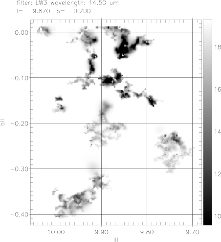 |
Figure 8: Reconstructed LW3 image of the 9.85-0.20 field |
| Open with DEXTER | |
m.
By choosing the reconstructed objects we lose some details, but this also
smoothes out part of the noise.
The aspect ratio is defined as:
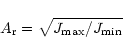
 is the largest principal moment of inertia
and
is the largest principal moment of inertia
and
 the smallest.
Aspect ratios around 1 are representative of roughly
spherical objects while larger ratios characterise
elongated shapes.
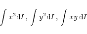
To obtain the moments of inertia, we calculate the
inertia centre of the object, then the three moments:
the smallest.
Aspect ratios around 1 are representative of roughly
spherical objects while larger ratios characterise
elongated shapes.
To obtain the moments of inertia, we calculate the
inertia centre of the object, then the three moments:
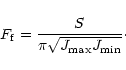
The filling factor is defined by:
As shape indicator, we use the parameter  :
:
 is equal to 1 for a
square,
is equal to 1 for a
square,
 for a rectangle of length
n and width 1,
for a rectangle of length
n and width 1,
 for n disconnected squares.
The histograms of the 4 parameters S,  ,
,
 and
are displayed in
Figs. 9 and 10, for the 3
threshold values.
and
are displayed in
Figs. 9 and 10, for the 3
threshold values.
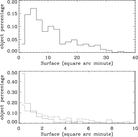 |
Figure 9: Clouds surface. Full line: 1 MJy sr-1 threshold. Dotted line: 3 MJy sr-1 threshold. Dashed line: 5 MJy sr-1 threshold |
| Open with DEXTER | |
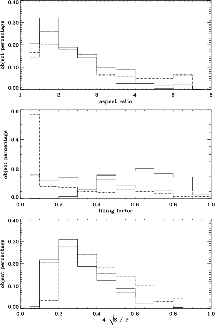 |
Figure 10: Aspect ratio, filling factor and shape indicator of the clouds, for three different thresholds (see Fig. 9) |
| Open with DEXTER | |
The cloud surfaces, S, vary from less than 1 to over 30 square arcmin and depend strongly on the threshold. For the lowest threshold value, the typical surface is about 5 to 20 square arcmin whereas it is barely 1 square arcmin for the largest threshold. This shows that the clouds are not uniform but present small denser parts and broad diffuse parts.
The aspect ratio ranges from 1 to 6 and the peak of the distribution is around 1.5-2. The aspect ratio increases with the threshold value. The condensed structures are thus mostly elongated. This does not exclude sheets, which are more easily detected in absorption when seen edge on.
The filling factor depends a lot on the threshold value. Its typical value is about 0.5, 0.2 and 0.1 respectively for the three thresholds considered. The denser parts do not fill the surface, meaning that the dark structures contain more than one single dense part. Therefore the dark objects present an internal structure composed by a broad envelope with few denser parts inside.
The typical value of
is 0.2, meaning that the objects are very
fragmented with a lot of contours. 25 isolated squares or a rectangle
of aspect ratio 100 would be necessary to get the same value of
.
Its value increases somewhat when larger thresholds are
considered, which is consistent with the picture of few small dense
cores in a more diffuse envelope. As shown in Teyssier et al. (2001),
these objects indeed turn out to be the most condensed cores of giant
molecular clouds located between the Sun and the galactic
"tangent point'' (position where the line of sight is tangent to a galactic
circle, roughly mid way through the disk). We shall now see that many
of them indeed lie quite deep in the disk.
m. Confusion on the contrary might prevent
some detections in the most populated (brightest) areas. The number
density of these condensed objects seems anyway to follow the galactic
distribution of young population components as traced e.g. in CO
surveys: peak in the centre and an excess around
 corresponding to the longest lines of sight through the molecular ring
(Solomon et al. 1979; Cohen et al. 1980; Sanders et al. 1984). The
apparent rough proportionality between the dark clouds number density
and the average mid-IR background intensity, although not astounding,
cannot be straightforwardly interpreted.
corresponding to the longest lines of sight through the molecular ring
(Solomon et al. 1979; Cohen et al. 1980; Sanders et al. 1984). The
apparent rough proportionality between the dark clouds number density
and the average mid-IR background intensity, although not astounding,
cannot be straightforwardly interpreted.
Follow-up studies based on molecular spectroscopy (Teyssier et al. 2001) and near infrared IJK-band star counts agree on distance evaluations in the range 2-8 kpc. A significant fraction of the dark cores detected belongs to the molecular ring or to innermore regions, in agreement with the conclusion of the MSX galactic survey (Egan et al. 1998).
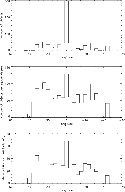 |
Figure 11:
Distribution of the dark objects seen
in LW3 and in LW9 with galactic longitude
for
 .
First top histogram: no normalisation is
applied. Second histogram: normalisation by the
observed surface. For comparison the average background intensity
in LW3 and
LW9 filters has been displayed in the lower panel .
First top histogram: no normalisation is
applied. Second histogram: normalisation by the
observed surface. For comparison the average background intensity
in LW3 and
LW9 filters has been displayed in the lower panel |
| Open with DEXTER | |
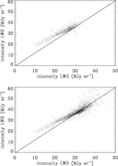 |
Figure 12:
Scatter diagram of LW2 versus LW3 intensity
for the dark feature DF+9.85-0.05.
In the upper panel pixels within the mask
given by the wavelet extraction (threshold equal to
2 MJy sr-1) have been used whereas
the bottom panel includes all pixels in a larger rectangular
area encompassing the object.
The straight line represents the average colour (ratio 1.2) |
| Open with DEXTER | |
m
brightness fluctuations within the boundaries of each of the dense
cores of the LW2-LW3 catalogue. The Galactic Centre samples will be
considered separately (Sect. 6). Average estimates of the opacity
ratio
 are derived from the
correlation of these brightness fluctuations. Absolute opacities will
be derived for a few clouds in Sect. 5.
are derived from the
correlation of these brightness fluctuations. Absolute opacities will
be derived for a few clouds in Sect. 5.
After an accurate image registering using the
ISOGAL star catalogues, scatter diagrams of 7 and 15 m
intensities are plotted for all objects. The examples given in
Fig. 12 show that the dark pixels (upper panel)
significantly depart from the average intensity correlation
represented by the straight line. The second plot (bottom panel) indeed includes a
number of pixels surrounding the dark object. These external pixels
follow the average correlation (7 to 15 m ratio 1.2,
see Fig. 3).
The departure of the dark pixels from the average correlation is interpreted as inverse reddening ("blue-ing'') due to differential absorption in the 2 wavelength bands. The magnitude of the effect implies that the attenuation in both bands is different and significant.
We assume in the following that the pixel intensity fluctuations,
within the boundaries of a given object I i (i=1 for the 15 m
filter, i=2 for the 7 m filter) are dominated by fluctuations of
the absorption within the object, and so define a non absorbed
intensity
 that will be estimated with a median filter in a
 strip around the object.
This strip is extended if needed, in order to include a minimum of 5000
pixels not belonging to the cloud.
The definition of the pixel dependent contrast follows, for each
filter:
strip around the object.
This strip is extended if needed, in order to include a minimum of 5000
pixels not belonging to the cloud.
The definition of the pixel dependent contrast follows, for each
filter:
 |
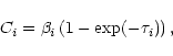
(1) |
m contrast
correlation in the dark objects, we simply model the pixel intensity
as superposition of emission from behind the cloud,
 ,
cloud
opacity
,
cloud
opacity  and emission from material in front of the cloud,
 .
Additional absorption, behind or in front of the cloud is ignored at
this stage. The pixel intensity then simply writes:
.
Additional absorption, behind or in front of the cloud is ignored at
this stage. The pixel intensity then simply writes:
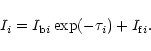 |
(2) |
and
are uniform over the cloud, the intensity
fluctuations being attributed to fluctuations of .
Under these assumptions
 and the "darkness'' contrast writes:
 ,
is at most equal to 1.
The contrast C i always satisfies C
,
is at most equal to 1.
The contrast C i always satisfies C
 .
The uniformity
of the diffuse emission colour shown by
Figs. 3 and 4 favours the
additional assumption
.
The uniformity
of the diffuse emission colour shown by
Figs. 3 and 4 favours the
additional assumption
 .
These simple relations
are now used to constrain the values of
for the LW2-LW3
sample. Part of the assumptions will be relaxed in later sections.
.
These simple relations
are now used to constrain the values of
for the LW2-LW3
sample. Part of the assumptions will be relaxed in later sections.
m opacity ratio
m contrast ratio
m darkness contrast ratio writes, in the simple
workframe just introduced:
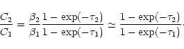 |
(4) |
 ,
,
 ,
if
,
if
 ,
,
 .
.
In order to boost the signal to noise ratio, the calculation of the
contrast ratio is achieved using larger pseudo-pixels.
Pseudo pixels are averages
of 10 pixels, grouped in order of decreasing contrast at 15 m.
The resulting values are noted <Ci> (i=1, 2). The distribution
of these values and of their ratio are shown in Fig. 13:
restricted to the darkest pseudo-pixel of each object (left panels)
or including up to 40 pseudo-pixels per object (right panels).
The distributions of <C1> and <C2> peak respectively
around 0.3 and 0.25.
As <Ci> is smaller than the opacity ,
we can infer that the maximum opacity
for most of the dark objects is greater than
0.3 at 14
and greater than 0.2 at 7
.
Some of them have values of <C1> and <C2> larger than 0.5
indicating probably more massive and/or closer objects.
A few examples are studied in the next section.
The histograms of the 7 to 15 m contrast ratio relatively sharply
peak around
implying an opacity ratio  smaller than 0.8. Let us also remark that the
full width at half maximum of the <C1> histograms
is about 0.15 whereas it is about 0.1 for <C2>.
The ratio of the two is expected to be at first order
roughly proportional to ,
thus consistent
with an upper limit around 0.75.
smaller than 0.8. Let us also remark that the
full width at half maximum of the <C1> histograms
is about 0.15 whereas it is about 0.1 for <C2>.
The ratio of the two is expected to be at first order
roughly proportional to ,
thus consistent
with an upper limit around 0.75.
m opacity ratio
 and 15 m opacities
 .
Assuming that the actual
.
Assuming that the actual  values are in the
range [0.5, 1], a prediction of
can be made from
Eq. (5), under the assumption
values are in the
range [0.5, 1], a prediction of
can be made from
Eq. (5), under the assumption
 ,
namely
,
namely
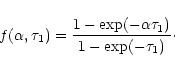
 as shown
in Fig. 14.
as shown
in Fig. 14.
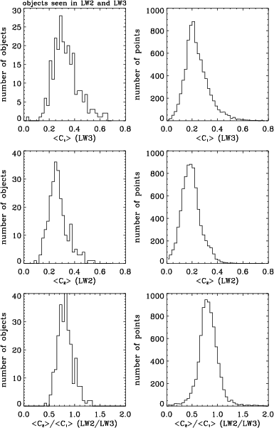 |
Figure 13: Histograms of < C1 > (LW3), < C2 > (LW2) and < C2 > / < C1 >. Left panels: darkest values obtained in each cloud (see text). Right panels: all values obtained (limited to 40) in each cloud |
| Open with DEXTER | |
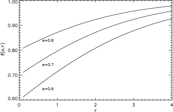 |
Figure 14:
f plotted as a function of
for three values of
|
| Open with DEXTER | |
 is
expected. A similar conclusion was reached by Abergel et al. (1998)
for a dense core in the solar neighbourhood.
Contrarily, it is less consistent with the
observational results of Lutz (1998) who used hydrogen
recombination lines to constrain the extinction law at
mid-infrared wavelengths towards the Galactic center.
His results lead to a larger opacity ratio
is
expected. A similar conclusion was reached by Abergel et al. (1998)
for a dense core in the solar neighbourhood.
Contrarily, it is less consistent with the
observational results of Lutz (1998) who used hydrogen
recombination lines to constrain the extinction law at
mid-infrared wavelengths towards the Galactic center.
His results lead to a larger opacity ratio
 -1.1.
It would be interesting to better constrain our estimate of
.
This will be attempted on individual
objects, refining on the non-linear dependence of <C 2> with <C 1>.
-1.1.
It would be interesting to better constrain our estimate of
.
This will be attempted on individual
objects, refining on the non-linear dependence of <C 2> with <C 1>.
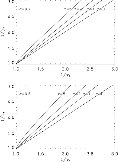 |
Figure 15:
 vs. vs.
 for
equal
to 0.6 and 0.7 and
for
equal
to 0.6 and 0.7 and
 equal to 0.1, 1, 2, 5
 |
| Open with DEXTER | |
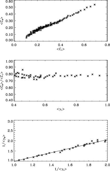 |
Figure 16:
Plot of <C2> vs. <C1>,
<C2> / <C1> vs.
 , ,
 vs. vs.
 for DF+09.85-0.05
 |
| Open with DEXTER | |
Before turning to these objects, let us point out that 10% of the data points have contrast ratios smaller than 0.6, and 10% larger than 1, hence significantly different from the median value 0.8. Several explanations can be put forward:
 and
and
 ;
;
 )
due for example to diffuse extinction on the line of sight (see Sect. 6.3)
or to local emission with different colour;
itself.
)
due for example to diffuse extinction on the line of sight (see Sect. 6.3)
or to local emission with different colour;
itself.
 and the contrast ratio
C 2 / C 1 from
and the contrast ratio
C 2 / C 1 from
 to
to
 ,
with increasing opacities .
It
follows that the maximum relative variation of the contrast ratio
gives an upper limit to
irrespective of additional
assumptions on
.
Conversely, if
is
assumed to be known, the maximum relative variation of the contrast
ratios yields an estimate of the maximum opacity through the cloud.
,
with increasing opacities .
It
follows that the maximum relative variation of the contrast ratio
gives an upper limit to
irrespective of additional
assumptions on
.
Conversely, if
is
assumed to be known, the maximum relative variation of the contrast
ratios yields an estimate of the maximum opacity through the cloud.
| Coordinates (l, b) |
 |
 |
(
vs.
)
slope |
 : :
 ,
( ,
( , ,  ) ) |
 :
,
(, ) :
,
(, ) |
| (4.35, -0.05) | 0.42 | 0.34 |
 |
 ,
(0.43, 0.37) ,
(0.43, 0.37) |
 ,
(0.45, 0.42) ,
(0.45, 0.42) |
| (9.85, -0.02) | 0.67 | 0.50 |
 |
 ,
(1, 1) ,
(1, 1) |
 ,
(1.2, 1.3) ,
(1.2, 1.3) |
| (12.42, -0.15) | 0.52 | 0.36 |
|
 ,
(0.67, 0.55) ,
(0.67, 0.55) |
,
(0.82, 0.71) |
| (15.06, 0.08) | 0.67 | 0.52 |
 |
 ,
(0.73, 0.63) ,
(0.73, 0.63) |
 ,
(0.86, 0.87) ,
(0.86, 0.87) |
| (18.55, -0.15) | 0.47 | 0.3 |
 |
 ,
(0.54, 0.4) ,
(0.54, 0.4) |
 ,
(0.51, 0.38) ,
(0.51, 0.38) |
| (30.01, -0.40) | 0.36 | 0.26 |
|
,
(0.39, 0.31) |
,
(0.46, 0.44) |
We define a normalised contrast, equal to 1 at the darkest position:
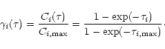 |
(6) |
 and
and  is shown in
Fig. 15 for different values of
is shown in
Fig. 15 for different values of
 ,
and for
and
.
The sensitivity on
is more obvious when using inverse contrasts,
adopted for these plots.
These simple behaviours are now used for examining 6 examples of
relatively good signal to noise ratio.
,
and for
and
.
The sensitivity on
is more obvious when using inverse contrasts,
adopted for these plots.
These simple behaviours are now used for examining 6 examples of
relatively good signal to noise ratio.
,
and
vs.
scatter diagram.
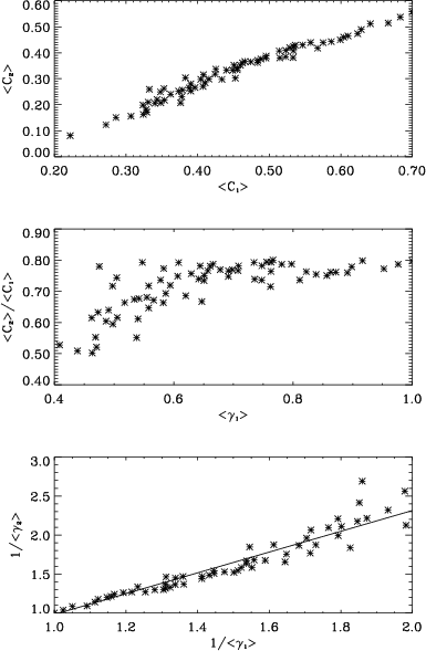 |
Figure 17: Same as Fig. 16 for DF+15.05+0.08 |
| Open with DEXTER | |
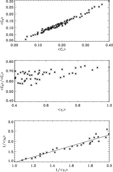 |
Figure 18: Same as Fig. 16 DF+30.00-0.39 |
| Open with DEXTER | |
In the three cases presented in
Figs. 16-18, as predicted by the model
(Fig. 14)
the ratio
<C2> / <C1> increases slightly with .
For DF+09.85-0.05 (Fig. 16)
the value of
<C2> / <C1> does not significantly increase.
Its value is 0.78
suggesting
 and
and
 .
For DF+15.05+0.08 (Fig. 17),
<C2> / <C1> varies
between less than 0.65 and 0.8
suggesting a value of
.
For DF+15.05+0.08 (Fig. 17),
<C2> / <C1> varies
between less than 0.65 and 0.8
suggesting a value of
 and a darker object
with
and a darker object
with
 .
For DF+30.01-0.40 (Fig. 18)
<C2> / <C1> ranges from 0.65 to less than 0.75.
This is compatible with a value of
and a value of
larger than 1.
.
For DF+30.01-0.40 (Fig. 18)
<C2> / <C1> ranges from 0.65 to less than 0.75.
This is compatible with a value of
and a value of
larger than 1.
These three special cases are in good agreement with a value
 ,
close to Draine & Lee's prediction ( 1984).
Most probably, the variations are due to
values of
,
close to Draine & Lee's prediction ( 1984).
Most probably, the variations are due to
values of
 .
.
Best estimates of
 ,
and are given in Table 1 for the 6 examples retained, assuming either
or
.
The accuracy of the slope estimates in the
vs.
diagrams is limited by the accuracy of the background
estimate. We use different methods to measure its value and evaluate
the accuracy of the slope estimates to be
,
and are given in Table 1 for the 6 examples retained, assuming either
or
.
The accuracy of the slope estimates in the
vs.
diagrams is limited by the accuracy of the background
estimate. We use different methods to measure its value and evaluate
the accuracy of the slope estimates to be
 .
.
The maximum 15
optical depths range from 1 to 3.5
(or maybe more, but the methods lack sensitivity to larger values)
for
and from less than 1 to 2.5 for
.
The values of
and
range
from 0.4 for DF+30.01-0.40 to 1
for DF+09.85-0.02. This suggests that DF+09.85-0.02
is the nearest cloud whereas DF+30.01-0.40 should
be the most distant one.
The
ratio is
consistently around 0.8 if
and 1 if
,
but
some variation is not unlikely (see Figs. 3 and 4).
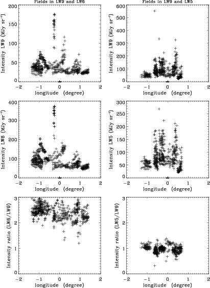 |
Figure 19:
Intensity (median value in a regions of
 pixels)
of the fields seen in LW9-LW6 (left panels)
and LW9-LW5 (right panels)
as a function of the Galactic longitude
pixels)
of the fields seen in LW9-LW6 (left panels)
and LW9-LW5 (right panels)
as a function of the Galactic longitude |
| Open with DEXTER | |
 at 7 m
from Lutz's extinction is 4-5 10-2,
yielding H column densities ranging from 0.25 to 1 1023cm-2 for solar neighbourhood conditions.
The value proposed by Draine & Lee is 1.5-2 10-2 which leads to column densities ranging
from 1 to 4 1023 cm-2.
These values are consistent with
most of the values given by Carey et al. (1998) except for
the clouds located in the Galactic Centre where
higher values (1024-1025 cm-2) are found
(see also Lis & Menten 1998; Lis et al. 1998).
at 7 m
from Lutz's extinction is 4-5 10-2,
yielding H column densities ranging from 0.25 to 1 1023cm-2 for solar neighbourhood conditions.
The value proposed by Draine & Lee is 1.5-2 10-2 which leads to column densities ranging
from 1 to 4 1023 cm-2.
These values are consistent with
most of the values given by Carey et al. (1998) except for
the clouds located in the Galactic Centre where
higher values (1024-1025 cm-2) are found
(see also Lis & Menten 1998; Lis et al. 1998).
3.5 arcmin)
in the fields of the second
and third groups as a function of the longitude.
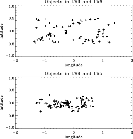 |
Figure 20: Position of the clouds seen in LW9-LW6 (upper panel) and LW9-LW5 (lower panel) |
| Open with DEXTER | |
It ranges from 30 to 150 MJy sr-1 for the second group
and from 50 to 200 MJy sr-1 for the third group.
The intensity variations are more important than for the first
observation group, the background is more structured.
The ratio between the intensities in the two bands,
LW9 and LW6, is about 2.5
whereas it is about 1 between the two bands LW9 and LW5 while it was
1.2 for the first observation group.
This is mostly due to the relative contribution of the 7.7 m PAH
feature to the emission measured in each of the 7 m filters.
The distribution in galactic coordinates
of the clouds belonging to the second and third
observation group
are shown in Fig. 20.
Clearly, the third observation group is nearer
to the Galaxy Centre than the second one.
The nearest clouds are located to about
0.2 from the Galaxy Centre.
The absorption properties of these clouds are now analysed in the same
way as shown in Sects. 4 and 5 for the clouds belonging to the first group.
from the Galaxy Centre.
The absorption properties of these clouds are now analysed in the same
way as shown in Sects. 4 and 5 for the clouds belonging to the first group.
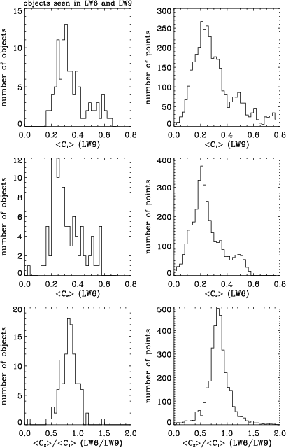 |
Figure 21: Same as Fig. 13 for the clouds observed with the filters LW9 and LW6 |
| Open with DEXTER | |
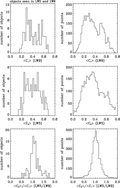 |
Figure 22: Same as Fig. 13 for the clouds observed with the filters LW9 and LW5 |
| Open with DEXTER | |
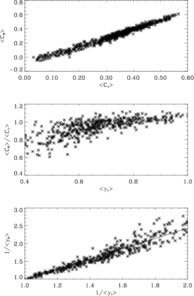 |
Figure 23: Same as Fig. 16 for DF-0.33+0.00 |
| Open with DEXTER | |
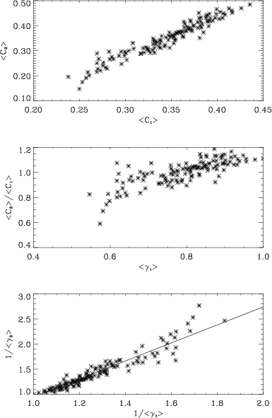 |
Figure 24: Same as Fig. 16 for DF+0.45+0.23 |
| Open with DEXTER | |
The histograms of <C1>, <C2>and <C2>/ <C1> for the second group are displayed in Fig. 21. They are similar to the histograms of the first group (Fig. 13) except that, due to large background intensities (Fig. 19) the distribution of < C1 > and < C2 > present larger wings.
The value of the ratio
<C2> / <C1> for
the second group is equal to
 .
It is a little higher than the value
found for the first group, but
not inconsistent with this wider band, wider area
value. Several explanations for this higher value will
be discussed in the next section.
.
It is a little higher than the value
found for the first group, but
not inconsistent with this wider band, wider area
value. Several explanations for this higher value will
be discussed in the next section.
.
Although massive clouds with larger opacity ( )
could explain a
value of
<C2> / < C1> equal to 0.9-1 (see Fig. 14),
it cannot explain that most of the points are above 1 except if
is significantly larger than 1. A simple way of
achieving such values without changing the colours of the dust
emission along the line of sight in an ad-hoc way, is to take
extinction along the line of sight into account.
Indeed in the direction of the Galactic Centre
opacities up to 1 are expected at 15
.
)
could explain a
value of
<C2> / < C1> equal to 0.9-1 (see Fig. 14),
it cannot explain that most of the points are above 1 except if
is significantly larger than 1. A simple way of
achieving such values without changing the colours of the dust
emission along the line of sight in an ad-hoc way, is to take
extinction along the line of sight into account.
Indeed in the direction of the Galactic Centre
opacities up to 1 are expected at 15
.
If we assume that the source function is constant along the line of sight,
and that the extinction in front of and behind the cloud are respectively
 and
and
 ,
the observed intensities write:
,
the observed intensities write:
 |
 |
||
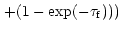 |
(7) |
,
the cloud opacity.
The
ratio then writes:
 |
 opacity ratio different from 1 will result into
ratios not equal to 1, even with the assumption
of a uniform source function.
Assuming again that
opacity ratio different from 1 will result into
ratios not equal to 1, even with the assumption
of a uniform source function.
Assuming again that
 ,
the corresponding
order of magnitude for
,
the corresponding
order of magnitude for
 is 1.1
and 1.2 for
is 1.1
and 1.2 for
 .
Thus, the contrast ratio
has to be divided by a factor 1.1 to 1.2 in order to correct its value
from the diffuse extinction. This leads to a typical value around
0.9 more consistent with first group clouds, although likely to have
higher optical depths. This would imply that most clouds of the
third group are further away from the Sun, hence really close
to the Galactic Centre.
.
Thus, the contrast ratio
has to be divided by a factor 1.1 to 1.2 in order to correct its value
from the diffuse extinction. This leads to a typical value around
0.9 more consistent with first group clouds, although likely to have
higher optical depths. This would imply that most clouds of the
third group are further away from the Sun, hence really close
to the Galactic Centre.
Alternative explanations might have been:
near the Galactic Centre that
could be due to the star contribution to the background
intensity in this region (the ratio
becomes significantly
different from 1). However this explanation is not supported
by the fact that we observe no systematic gradient
in the background colour ratio (Fig. 19);
itself resulting
from an evolution of the dust properties near the
Galactic Centre as for example a gradient of
the abundance ratio of
graphite and silicate particles which are
responsible for the
absorption respectively at 7 and 15 m.
Indeed, the corresponding opacity ratio derived with our model (
)
is in acceptable agreement with the value obtained from the extinction
measurement of Lutz (1998).
However, maximum opacity ratios can be derived from the relative
variation of
<C 2> / <C 1> within the boundaries of one cloud (see
Sect. 5). Two examples are shown (Figs. 23
and 24) which both imply
,
irrespective of
any additional assumption. This finding contradicts Lutz's (1998)
derivation of
.
An equivalent trend is shown by the
normalised contrast scatter diagrams, which exhibit slopes around 1.5,
inconsistent with
values close to 1.
vs.
curve equal to
 for DF-0.33+0.00 and
 for DF+0.45+0.23).
Using a multiresolution analysis,
we have extracted the dark features seen in absorption
and studied their morphology and location.
Although few data are available at longitudes
larger than 40,
the distribution is consistent with
the distribution of young components (see also Egan et al. 1998).
These dark clouds are condensed cores of galactic giant molecular clouds.
Near Infrared and radio follow-ups will refine this view.
We studied the cross-correlation of intensity fluctuations in both
7 and 15 m bands available.
A 7 to 15 m contrast ratio of
has been inferred for the
inner disk sample.
A simple model translates this ratio into a 7 to 15 m opacity
ratio of
in good agreement with the extinction curve calculated by
Draine & Lee (1984) but not consistent with the value obtained by Lutz (1998).
For two values (0.6 and 0.7) of the opacity ratio, we derived the maximum opacity
reached for six of these clouds. Typical values are
m bands available.
A 7 to 15 m contrast ratio of
has been inferred for the
inner disk sample.
A simple model translates this ratio into a 7 to 15 m opacity
ratio of
in good agreement with the extinction curve calculated by
Draine & Lee (1984) but not consistent with the value obtained by Lutz (1998).
For two values (0.6 and 0.7) of the opacity ratio, we derived the maximum opacity
reached for six of these clouds. Typical values are
 leading to H column densities ranging from
1-4 1023 cm-2 for solar neighbourhood conditions.
leading to H column densities ranging from
1-4 1023 cm-2 for solar neighbourhood conditions.
The contrast ratio for the clouds seen with
the narrower filters LW6 and LW9 and
located near the Galactic Centre (
 ,
)
is
whereas it is
for the clouds seen with the filters LW5 and LW9 and located at lower
latitude (
,
).
This last result is straightforwardly accounted for by diffuse
extinction along the line of sight and the fact that the clouds near
the Galactic Centre
are more massive than clouds of the inner disk.
These data are not consistent with Lutz's (1998) finding of a
significantly different mid Infrared extinction curve in the Galactic
Centre area.
,
)
is
whereas it is
for the clouds seen with the filters LW5 and LW9 and located at lower
latitude (
,
).
This last result is straightforwardly accounted for by diffuse
extinction along the line of sight and the fact that the clouds near
the Galactic Centre
are more massive than clouds of the inner disk.
These data are not consistent with Lutz's (1998) finding of a
significantly different mid Infrared extinction curve in the Galactic
Centre area.
Acknowledgements
The authors wish to thank Bill Reach for his decisive help in zodiacal emission estimates and Albert Bijaoui, Eric Slezac and Benoit Vandame for providing the MVM software. This work much benefitted from the involvement of the ISOCAM instrument team and of the ISOGAL team. Let them all be warmly thanked. We also thank Patrick Boissé for several stimulating discussions.