A&A 365, 301-313 (2001)
DOI: 10.1051/0004-6361:20000004
Real-time optical path difference compensation at the Plateau de
Calern I2T interferometer
B. Sorrente1 - F. Cassaing1 - G. Rousset1
- S. Robbe-Dubois2,3 - Y. Rabbia2
Send offprint request: B. Sorrente
1 - Office National d'Études et de Recherches Aérospatiales (ONERA),
DOTA, BP 72, 92322 Châtillon Cedex, France
2 - Observatoire de la Côte d'Azur, Fresnel Department, UMR 6528,
avenue Copernic, 06130 Grasse, France
3 - now at Université de Nice - Sophia Antipolis,
Laboratoire d'Astrophysique, UMR 6525, Parc Valrose,
06108 Nice Cedex 2, France
Received 6 January 1999 / Accepted 14 August 2000
Abstract
The fringe tracker system of the ASSI (Active Stabilization in Stellar
Interferometry) beam combining table at the I2T interferometer is described
and its performance evaluated. A new real-time algorithm for the optical path
difference (OPD) measurement is derived and validated. It is based on a
sinusoidal phase modulation whose amplitude is optimized. It also allows
automatic fringe detection at the beginning of an observation when scanning
the OPD. The fringe tracker servo-loop bandwidth is adjusted by a numerical
gain and ranges between 20 and 50 Hz in the reported experiments. On stars,
fringe-locked sequences are limited to 20 s due to fringe jumps. However, the
fringe tracker is able to recover the coherence area after a few seconds. Such
a fringe tracker operation can last more than one hour. A fringe tracking
accuracy of 85 nm is achieved for visibility ranging between 7 and 24%, a
turbulence coherence time of approximately 9 ms at 0.85  m, a Fried
parameter of around 14 cm at 0.5 m and an average light level of
100000 photoevents/s, (typically visual magnitude 2 in the conditions of the
experiment). Visibility losses are evaluated and are found to be mainly due to
turbulent wavefront fluctuations on the two telescopes and to the static
aberrations of the optical train. The measurements of OPD and angle of arrival
are reduced to derive turbulence parameters: the coherence time, the average
wind speed, the Fried parameter and the outer scale. Our estimations for the
outer scale range between 20 and 120 m, with an average value of the order of
40 m. Both OPD and angle of arrival data, obtained on 15 m baseline and a
26 cm telescope diameter respectively, are fully compatible with the same
modified Kolmogorov spectrum of the turbulence, taking into account a finite
outer scale.
m, a Fried
parameter of around 14 cm at 0.5 m and an average light level of
100000 photoevents/s, (typically visual magnitude 2 in the conditions of the
experiment). Visibility losses are evaluated and are found to be mainly due to
turbulent wavefront fluctuations on the two telescopes and to the static
aberrations of the optical train. The measurements of OPD and angle of arrival
are reduced to derive turbulence parameters: the coherence time, the average
wind speed, the Fried parameter and the outer scale. Our estimations for the
outer scale range between 20 and 120 m, with an average value of the order of
40 m. Both OPD and angle of arrival data, obtained on 15 m baseline and a
26 cm telescope diameter respectively, are fully compatible with the same
modified Kolmogorov spectrum of the turbulence, taking into account a finite
outer scale.
Key words: atmospheric effects - instrumentation: interferometers - methods:
data analysis -
methods: observational - techniques: interferometric
Author for correspondance: Sylvie.robbe-dubois@unice.fr
According to the Zernike-van Cittert theorem, the fringe visibility in a
stellar interferometer of baseline  is directly related to the object
spectrum value at the spatial frequency
is directly related to the object
spectrum value at the spatial frequency
 where
where  is the
observation wavelength. Since the baseline can reach several tens of meters,
long baseline interferometry has the ability to achieve very high resolution
(Labeyrie 1975). However, observations made from the ground are severely
limited by atmospheric turbulence (Roddier 1981). Such turbulence induces
wavefront disturbances over the telescopes, reducing the fringe visibility.
These distorsions are responsible for speckled images, image motion and
optical path difference (OPD) fluctuations. Turbulence effects can be fought
by speckle techniques, based on the recording of a long set of short exposure
data, or by real-time correction for better signal to noise ratio (SNR)
(Roddier & Léna 1984). Two modes can be distinguished for OPD correction. In the
coherencing mode, the requirement is to achieve OPD residuals smaller than the
coherence length, ensuring interference only in the short exposure data. In
the cophasing mode, the requirement is to achieve OPD residuals much smaller
than the wavelength, allowing long exposures. In case of large OPD residuals,
cophasing suffers from fringe jumps and requires some kind of coherencing to
track the central fringe. Only a few fringe tracker systems have been
implemented for stellar observations. The SUSI (Davis et al. 1995) or GI2T
(Koechlin et al. 1996) interferometers allow only coherencing. Cophasing (with
simultaneous coherencing) has only been used by the Mark III (Shao et al. 1988),
NPOI (Armstrong et al. 1998) or PTI (Colavita et al. 1999) interferometers.
is the
observation wavelength. Since the baseline can reach several tens of meters,
long baseline interferometry has the ability to achieve very high resolution
(Labeyrie 1975). However, observations made from the ground are severely
limited by atmospheric turbulence (Roddier 1981). Such turbulence induces
wavefront disturbances over the telescopes, reducing the fringe visibility.
These distorsions are responsible for speckled images, image motion and
optical path difference (OPD) fluctuations. Turbulence effects can be fought
by speckle techniques, based on the recording of a long set of short exposure
data, or by real-time correction for better signal to noise ratio (SNR)
(Roddier & Léna 1984). Two modes can be distinguished for OPD correction. In the
coherencing mode, the requirement is to achieve OPD residuals smaller than the
coherence length, ensuring interference only in the short exposure data. In
the cophasing mode, the requirement is to achieve OPD residuals much smaller
than the wavelength, allowing long exposures. In case of large OPD residuals,
cophasing suffers from fringe jumps and requires some kind of coherencing to
track the central fringe. Only a few fringe tracker systems have been
implemented for stellar observations. The SUSI (Davis et al. 1995) or GI2T
(Koechlin et al. 1996) interferometers allow only coherencing. Cophasing (with
simultaneous coherencing) has only been used by the Mark III (Shao et al. 1988),
NPOI (Armstrong et al. 1998) or PTI (Colavita et al. 1999) interferometers.
The "Active Stabilization in Stellar Interferometry'' (ASSI) table, developed
by the Office National d'Études et de Recherches Aérospatiales (ONERA)
aims to compensate in real-time for turbulence disturbances in the
"Interféromètre à 2 Télescopes'' (I2T) of the Observatoire de la
Côte d'Azur (OCA), France (Robbe et al. 1994). OPD and angle of arrival
fluctuations respectively are corrected by a fringe tracker and two star
trackers, one for each telescope. The first fringes were observed and
stabilized in June 1994 with an 11 m baseline.
The goals of our work were to implement the technologies relevant to optical
aperture synthesis and to demonstrate the performance of fringe tracking as a
function of observing conditions, i.e. the seeing and the visual magnitude
( )
of the observed star. The performance evaluations are coupled
to measurements of the spatial and temporal characteristics of the turbulence.
Atmospheric measurements previously were made by other stellar interferometers
(Mariotti & Di Benedetto 1984; Bester et al. 1992;
Buscher et al. 1995; Davis et al. 1995).
)
of the observed star. The performance evaluations are coupled
to measurements of the spatial and temporal characteristics of the turbulence.
Atmospheric measurements previously were made by other stellar interferometers
(Mariotti & Di Benedetto 1984; Bester et al. 1992;
Buscher et al. 1995; Davis et al. 1995).
This paper discusses the results obtained with the fringe tracker. For the
star trackers, see Robbe et al. 1997. In Sect. 2,
the I2T-ASSI interferometer and the fringe tracker are described. In
Sect. 3, two new algorithms for fringe detection and tracking are
presented and their noise performance given. An analysis of visibility losses
is performed in Sect. 4. The experimental visibilities are
compared with the expected values. Section 5 deals with the
fringe tracking results in the laboratory and the sky. In
Sect. 6, we report the estimations of the atmospheric
coherence time and the outer scale deduced from temporal power spectra and
variances of OPD and angle of arrival fluctuations.
2 Description of the instrument
I2T is a stellar interferometer including two movable 26 cm diameter
telescopes mounted on rail tracks on a north-south baseline
(Koechlin & Rabbia 1985). Accessible baselines span from 10 to 140 m. Light is
sent through the air towards a central laboratory where the two beams are
combined by ASSI for visibility measurements in a scientific instrument. The path
length variation due to the Earth's rotation is compensated by a cat's eye
delay line inserted in the south arm. A static delay line in the north arm
ensures symmetry.
Early I2T operations showed the limitations of visual fringe search and
calibration of turbulence-degraded visibility (Koechlin 1985). It was
decided in 1988 to equip I2T with the ASSI table dedicated to automatic fringe
detection and fringe stabilization (Damé et al. 1988;
Sorrente et al. 1991). Its design
was partially upgraded before the instrument was set up at I2T in 1993
(Sorrente et al. 1994).
The ASSI table has already been presented by Robbe et al. 1997.
It mainly involves two servo-tracking systems dedicated to the angle of
arrival correction of the two telescopes, and one dedicated to OPD correction
(Fig. 1). The star trackers share the visible light with a
scientific dedicated instrument in the
 spectral range.
A photon-counting quad cell detector (star sensor), alternatively fed by each
arm of the interferometer, generates the error signals used to command the
tip-tilt mirrors. The system and its performance have been fully described in
a previous paper (Robbe et al. 1997): an accuracy of
spectral range.
A photon-counting quad cell detector (star sensor), alternatively fed by each
arm of the interferometer, generates the error signals used to command the
tip-tilt mirrors. The system and its performance have been fully described in
a previous paper (Robbe et al. 1997): an accuracy of  0.24 arcsec has been
achieved for a light level of 50000 photoevents/s (typically
0.24 arcsec has been
achieved for a light level of 50000 photoevents/s (typically
 )
and
)
and  10 cm at 0.5 m, where r0 is the Fried
parameter. The three servo-systems are driven by a 486/25 MHz Personal
Computer (PC), allowing data acquisition from the star and fringe trackers and
providing an user interface.
10 cm at 0.5 m, where r0 is the Fried
parameter. The three servo-systems are driven by a 486/25 MHz Personal
Computer (PC), allowing data acquisition from the star and fringe trackers and
providing an user interface.
The scientific instrument is based on dispersed Young-type fringes, providing
a two dimensional OPD-wavelength interferogram. This fringe pattern is
recorded on a photon-counting camera with an exposure time of 20 ms
and then 2-D Fourier transformed to extract the visibility.
2.2 The fringe tracker
Once the two beams are tilt-stabilized, their red component (
 m)
is sent towards the fringe sensor. The purpose of the fringe tracker is first
to localize the coherence area and then to compensate for the OPD between the
beams, induced by both atmospheric turbulence and metrology errors.
m)
is sent towards the fringe sensor. The purpose of the fringe tracker is first
to localize the coherence area and then to compensate for the OPD between the
beams, induced by both atmospheric turbulence and metrology errors.
To measure phase and visibility, a method widely used is to generate a known
phase modulation in the interferometer and to synchronously demodulate the
intensity variations. In stellar interferometry, the measurement time must be
short enough to freeze the fringe motion induced by atmospheric turbulence (a
few milliseconds in the visible). The magnitude of the observed objects
requires high efficiency detectors and wide band observation. These
constraints lead to the choice of a coaxial beam combination with sinusoidal
temporal phase modulation and a photon-counting avalanche photodiode (APD),
manufactured by EG&G, as a single-pixel detector.
In the fringe sensor (Fig. 1), the two afocal beams are
superimposed by a beam splitter cube in a flat-tint mode, in a pupil plane,
as in the Mark III interferometer (Shao et al. 1988). One of the two complementary
outputs is used for interference state measurement, with the APD. A filter
allows selection of the spectral bandpass. A camera for diagnostic purpose,
such as pupil lateral positioning, is set up at the other output. In the north
arm of the fringe sensor, a mirror mounted on a piezoelectric (PZT) actuator
induces a 280 Hz OPD modulation. This PZT is operated in open-loop conditions, but its
transfer function is measured with an internal calibration source before
observation. Real-time visibility and phase measurements are obtained by
demodulation of the APD signal (described in Sect. 3) during the
observation. A single interrupt-driven routine in the PC is in charge of PZT
driving modulation, APD counter reading, demodulation and control of the OPD
correction device, ensuring simple and perfect synchronization.
A first-order integral controller with adjustable gain is used to derive the
OPD command from the phase measurements (Appendix A). The numerical
loop-gain is adjusted by the observer according to the observing conditions
(light level and turbulence) in order to minimize the OPD residual variance.
However, an automatic procedure would have been much more efficient to obtain
the best optimization. The correction device is a two-stage delay line,
including a roof mirror mounted on a 8
 mechanical
stroke PZT actuator (fast delay line) and a 10 mm micropositioning
translation stage. The correction signal is sent to the PZT actuator. When the
PZT elongation exceeds a threshold value, the translation stage is used
for desaturation.
mechanical
stroke PZT actuator (fast delay line) and a 10 mm micropositioning
translation stage. The correction signal is sent to the PZT actuator. When the
PZT elongation exceeds a threshold value, the translation stage is used
for desaturation.
The visibility measured by the fringe sensor (Sect. 3) is used
for fringe detection by comparison with a threshold value selected by the
observer and based on the visibility level measured at large OPD (incoherent
measurement). The fringe detection process works continuously as the OPD is
linearly scanned by the translation stage. The integration time is set
according to the coherence length  of the fringe pattern and the
scan speed. Typical values are
of the fringe pattern and the
scan speed. Typical values are
 and a few
 ,
respectively, allowing an integration time of a few
seconds. If the visibility estimate increases above the alert threshold during
the OPD scan, then the scan is stopped. A new visibility estimate, with a
longer integration time, is performed. Comparison with another threshold, set
for these new conditions, allows the system to decide whether fringes are
actually there or not. In case of fringe detection, the servo tracking is
automatically switched on, otherwise the scan resumes.
,
respectively, allowing an integration time of a few
seconds. If the visibility estimate increases above the alert threshold during
the OPD scan, then the scan is stopped. A new visibility estimate, with a
longer integration time, is performed. Comparison with another threshold, set
for these new conditions, allows the system to decide whether fringes are
actually there or not. In case of fringe detection, the servo tracking is
automatically switched on, otherwise the scan resumes.
3 Visibility and phase measurement technique
The spectral bandwidth of the source and fringe sensor produces the following
interferogram:
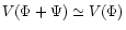
![\begin{displaymath}I(\Psi)=I_0 \left[ 1 + V(\Phi+\Psi)\cos(\Phi+\Psi) \right]
\end{displaymath}](/articles/aa/full/2001/02/aads1678/img27.gif) |
(1) |
where I is the measured intensity, I0 the mean intensity,  the
visibility.
the
visibility.  is the phase related to the position of the fringes
proportional to the OPD between the two telescopes, and
is the phase related to the position of the fringes
proportional to the OPD between the two telescopes, and  the phase
modulation. For monochromatic light, V is independent of
and the
interferogram can be detected with small amplitude (
the phase
modulation. For monochromatic light, V is independent of
and the
interferogram can be detected with small amplitude (
 )
modulation. For polychromatic light, the fringe pattern has an envelope: Vis high only within the coherence area, and null outside.
)
modulation. For polychromatic light, the fringe pattern has an envelope: Vis high only within the coherence area, and null outside.
In the cophasing mode, assuming that the modulation amplitude is much smaller
than the coherence length, the polychromatic interferogram can be approximated
by a monochromatic interferogram of visibility
 .
Equation (1) then becomes:
.
Equation (1) then becomes:
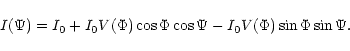 |
(2) |
The modulated intensity is thus the sum of the incoherent intensity offset and
two interferometric signals, proportional to the known waveforms  and
and  .
By linear demodulation, it is possible to estimate I0 and
the two fringe quadratures
.
By linear demodulation, it is possible to estimate I0 and
the two fringe quadratures
 and
and
 ,
from which fringe parameter estimation is straightforward, the phase being
measured modulo
,
from which fringe parameter estimation is straightforward, the phase being
measured modulo  .
To allow a high modulation frequency, a continuous OPD
modulation is most often used, while pulses delivered by the photon-counting
detector are integrated in K temporal buckets.
.
To allow a high modulation frequency, a continuous OPD
modulation is most often used, while pulses delivered by the photon-counting
detector are integrated in K temporal buckets.
Taking advantage of the orthogonality of the trigonometric functions, a
triangle OPD modulation of amplitude
is usually chosen, followed by
a Digital Fourier Transform of the K samples (DFTK). This is the case of
the so-called ABCD algorithm with K=4 intensity buckets per modulation
period (Shao et al. 1988).
3.1 Noise propagation for demodulation algorithms
Fringe parameter estimation is limited by photon noise. Noise
propagation for the phase and visibility estimators is an intrinsic
characteristic of each algorithm derived from the modulation function .
Except for the DFTK algorithm, noise propagation for visibility and phase
estimators depends on .
By the choice of the modulation function ,
it is possible for a given phase position
to reduce noise in the
estimated phase while increasing noise in the visibility. Such a strategy is,
of course, welcome for a fringe tracker. Cophasing performance is given by the
standard deviation
 of the phase estimator at
  .
When
.
When
 :
:
 |
(3) |
where N is the number of photoevents per modulation period and M is the
number of averaged modulation periods.  is a numerical coefficient
depending on the modulation .
is a numerical coefficient
depending on the modulation .
Visibility estimators, based on the squared amplitude of the signal, are
biased. A V2 estimator (denoted G2, Eq. (5) in
Sect. 4) is preferred to a V estimator since it can be unbiased
even when V=0. For fringe search, the figure of merit is the visibility
noise out of the coherence area. In this case for any algorithm, we have
(Cassaing et al. 1995):
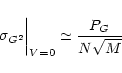 |
(4) |
where PG is a numerical coefficient depending on the modulation .
It
can be shown that the DFTK algorithm is the one with the minimum visibility
noise. Since the total number of photoevents involved is NM,
Eq. (4) shows that it is necessary for the fringe search to
increase as much as possible the number of photoevents per modulation period.
With continuous modulations, the OPD variation during the integration is
equivalent to a blur, reducing the contrast of the detected interferogram.
When limited by photon noise, it is thus more efficient to often read or
sample the detector signal ( )
to reduce the visibility loss
)
to reduce the visibility loss  .
For
the DFTK algorithm,
.
For
the DFTK algorithm,
 ,
,
 and
and
 .
For ABCD,
.
For ABCD,
 and
PG=4.44.
and
PG=4.44.
Other sources of noise on V and
are related to the turbulence
perturbations on the two apertures: the high order wavefront phase distorsions
(higher than OPD) are not negligible because in our experiments r0 is
always smaller than D, the telescope diameter. Scintillation also
contributes to the noise because such intensity fluctuations cannot be
distinguished from the signal resulting from the fringe temporal modulation.
The correlation length of the intensity fluctuations
 is of
the order of 10 cm for a turbulence altitude
is of
the order of 10 cm for a turbulence altitude
 km (Fante 1975).
The aperture averaging effect is therefore much lower for the I2T than for
large telescopes (Roddier 1981).
km (Fante 1975).
The aperture averaging effect is therefore much lower for the I2T than for
large telescopes (Roddier 1981).
3.2 SIMONE algorithm
The formalism of Sect. 3 can be applied to a sinusoidal
modulation
 .
There is no simple closed-form expression
for noise coefficients. But assuming a large K value, required for best
performance as previously shown,
and PG can be closely
approximated by the asymptotic case
.
There is no simple closed-form expression
for noise coefficients. But assuming a large K value, required for best
performance as previously shown,
and PG can be closely
approximated by the asymptotic case
 .
For best tracking, the
minimum value
.
For best tracking, the
minimum value
 is reached with a modulation amplitude m=1.91,
i.e. 0.6;
but then PG is 21% worse than with the DFT
is reached with a modulation amplitude m=1.91,
i.e. 0.6;
but then PG is 21% worse than with the DFT algorithm.
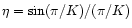
Other interesting values are when J0(m)=0 (J0 being the Bessel function
of the first kind): the waveforms 1,
and
are then
orthogonal (Cassaing 1997). Demodulation is therefore easily achieved
using these normalized waveforms. Although not used elsewhere to our
knowledge, open loop phase and visibility estimations are possible with
sinusoidal modulation. We chose the first root of J0 (m=2.40, i.e.
roughly 0.75)
and called this algorithm SIMONEK (Sinusoidal
Integrated Modulation on ONE fringe). We used K=16 buckets per modulation
period for the sinusoid generation and the intensity demodulation, so that
 .
Noise propagation coefficients for SIMONE
are
.
Noise propagation coefficients for SIMONE
are
 and
PG=4.36. SIMONE
is therefore 10% better for
phase tracking but 9% worse for fringe search than the DFTalgorithm. The SIMONE algorithm provides good noise behavior, very
similar or even better than the ABCD algorithm. An advantage of SIMONE is
that high frequency sinusoidal modulation is much simpler to implement in the
modulating device than triangle modulation. We used this single algorithm for
fringe search and tracking.
and
PG=4.36. SIMONE
is therefore 10% better for
phase tracking but 9% worse for fringe search than the DFTalgorithm. The SIMONE algorithm provides good noise behavior, very
similar or even better than the ABCD algorithm. An advantage of SIMONE is
that high frequency sinusoidal modulation is much simpler to implement in the
modulating device than triangle modulation. We used this single algorithm for
fringe search and tracking.
3.3 MAXSIM algorithm
Since the amplitude of the phase perturbation to be corrected for can reach a
few tens of fringes, whereas the rejection is limited by photon noise, phase
residuals may go beyond
![$]-\pi,\pi]$](/articles/aa/full/2001/02/aads1678/img59.gif) .
This introduces phase wrapping and
fringe jumps with cophasing estimators. Coherencing estimators, based on a
polychromatic analysis, are then required. If the modulation amplitude is
larger than
but smaller than ,
the envelope can be
approximated by its local slope (Cassaing 1997). Reporting the first
order Taylor expansion
.
This introduces phase wrapping and
fringe jumps with cophasing estimators. Coherencing estimators, based on a
polychromatic analysis, are then required. If the modulation amplitude is
larger than
but smaller than ,
the envelope can be
approximated by its local slope (Cassaing 1997). Reporting the first
order Taylor expansion
 in
Eq. (1) allows the measurement of
in
Eq. (1) allows the measurement of
 in addition
to the phase measurement, as described in Sect. 3, and thereby
the identification of the central fringe position. Therefore, with a
sinusoidal modulation of amplitude between
and ,
it is
possible to simultaneously derive a cophasing and a coherencing estimator. If
m is a root of J0, a visibility estimator can also be simply derived. We
used this algorithm with m=11.79, i.e. 3.75,
a third of the
coherence length, and called it MAXSIM. Noise propagation coefficients for
MAXSIM are similar to those of the DFT algorithm when the modulation amplitude
for both is large. But in this case, the visibility is reduced because of the
chromatic envelope degrading the phase measurement performance. So in
Sect. 5, we will show that MAXSIM was successful in the
laboratory but failed on the sky.
in addition
to the phase measurement, as described in Sect. 3, and thereby
the identification of the central fringe position. Therefore, with a
sinusoidal modulation of amplitude between
and ,
it is
possible to simultaneously derive a cophasing and a coherencing estimator. If
m is a root of J0, a visibility estimator can also be simply derived. We
used this algorithm with m=11.79, i.e. 3.75,
a third of the
coherence length, and called it MAXSIM. Noise propagation coefficients for
MAXSIM are similar to those of the DFT algorithm when the modulation amplitude
for both is large. But in this case, the visibility is reduced because of the
chromatic envelope degrading the phase measurement performance. So in
Sect. 5, we will show that MAXSIM was successful in the
laboratory but failed on the sky.
4 Visibility losses of the I2T-ASSI interferometer
In the fringe tracker system, a pupil plane coaxial beam combination is used
and the flat tint is recorded using a short exposure. This allows only one
component of the object spectrum to be measured at
,
leading to
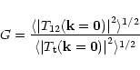
the visibility estimator G defined as (Rousset et al. 1991):
 |
(5) |
where
 represents the ensemble average, T12 is the
intercorrelation of the fields of the two apertures,
represents the ensemble average, T12 is the
intercorrelation of the fields of the two apertures,  the
transfer function of one telescope and
the
transfer function of one telescope and  the spatial frequency.
In the scientific instrument, the fringes are obtained by a multiaxial beam
combination in a focal plane and then are recorded using a short exposure. In
the data reduction process the spatial information is averaged over the
fringe peak. Therefore, the measured visibility corresponds to the definition
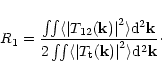
of R1 introduced by Roddier & Léna (1984):
 |
(6) |
The R1 estimator is well adapted to a single mode interferometer, i.e. D <
r0. This does not exactly correspond to our observing conditions. A new
multimode visibility estimator was recently proposed for multiaxial and short
exposure modes with large apertures ( )
(Mourard et al. 1994). However,
this estimator is not easily applicable to the I2T interferometer because the
telescope diameter is only slightly larger than r0. For the purpose of the
comparison of the different visibilities we define the estimator
)
(Mourard et al. 1994). However,
this estimator is not easily applicable to the I2T interferometer because the
telescope diameter is only slightly larger than r0. For the purpose of the
comparison of the different visibilities we define the estimator
 (equal to 1 when there is no aberration).
4.2 Analysis of the visibility losses
Various factors affect the fringe visibility in the interferometer
(Cassaing et al. 1996; Robbe 1996).
Atmospheric turbulence is the factor
which theoretically most affects the visibility. The different
contributors are:
- High order wavefront perturbations other than tip-tilts and OPD. We use
a numerical simulation to evaluate their effect on the estimators G and
R2. Neglecting scintillation, we generate 1024 turbulent phase wavefronts
for each pupil using the simulation tool of Rousset et al. (1991). Each
wavefront, j, is a linear combination of 230 Zernike polynomials
Zi(
 ). The Zernike expansion coefficients
ai(j) are Gaussian
random variables obeying Kolmogorov statistics. The variances,
). The Zernike expansion coefficients
ai(j) are Gaussian
random variables obeying Kolmogorov statistics. The variances,
 ,
behave as
(D/r0)5/3;
,
behave as
(D/r0)5/3;
- Tip-tilt residuals. Tips and tilts are assumed to be uncorrelated
between the two telescopes. In order to take into account the angle of arrival
correction brought by the ASSI table, the temporal power spectrum of the tip
and tilt modes (see Fig. C.1 for an outer scale L0=40 m) is
filtered by the transfer function of the star tracker (Robbe et al. 1997),
assuming that this process is free from noise propagation. The results are
added to the above computed wavefronts in order to derive T12 and
;
- OPD residuals. Because R2 and G are short exposure estimators, they
are theoretically not affected by OPD residuals left by the fringe tracker.
For G, the exposure is very short (3 ms), while much longer for R2 (20 ms).
From the temporal power spectrum of the OPD (Fig. C.1,
for L0=40 m) and the filtering due to the 20 ms exposure of the scientific
instrument and the transfer function of the fringe tracker
(Fig. 6), the high frequency OPD variance
 can be computed. The R2 visibility loss is estimated by
 (Conan & Rousset 1995) to a value of
0.97;
(Conan & Rousset 1995) to a value of
0.97;
- Scintillation effects (not quantified). Visibility noises are due to
intensity fluctuations on the two apertures.
Estimators G and R2 are then computed for various values of D/r0 using
Eqs. (5) and (6). Figure 2 presents the results
of the simulations. At large D/r0, R2 tends to
 ,
as
theoretically predicted (Roddier & Léna 1984). G quickly decreases with an
increase in D/r0 for
,
as
theoretically predicted (Roddier & Léna 1984). G quickly decreases with an
increase in D/r0 for
 ,
i.e. when the first turbulence
aberrations become significant in the visibility loss. For larger D/r0, its
value is low and still decreases. Because turbulence aberrations degrade the
transfer function
,
i.e. when the first turbulence
aberrations become significant in the visibility loss. For larger D/r0, its
value is low and still decreases. Because turbulence aberrations degrade the
transfer function
 for
for
 but has no impact on
the central value
but has no impact on
the central value
 ,
the degradation of
,
the degradation of
 is partly compensated in R2 while it is not the case
in G according to Eqs. (5) and (6). Therefore, R2 is
less sensitive to the turbulence aberrations than G (as shown in
Fig. 2).
is partly compensated in R2 while it is not the case
in G according to Eqs. (5) and (6). Therefore, R2 is
less sensitive to the turbulence aberrations than G (as shown in
Fig. 2).
![\begin{figure}
\par\includegraphics[width=8cm,clip]{ds1678F2.eps}\end{figure}](/articles/aa/full/2001/02/aads1678/Timg80.gif) |
Figure 2:
Variation of the visibility estimators versus D/r0 - tip-tilt
corrected by ASSI but with residuals included. No OPD residuals |
| Open with DEXTER |
The second important factor is the effect of the static aberrations of the
instrument. The aberrations of the optical train of the combining table, the
delay-lines and the telescopes were measured with a Shack-Hartmann wavefront
sensor, set up at different positions in the interferometer. From each set of
measurements, the tip, tilt and defocus modes of the wavefront were filtered
for visibility estimation. These modes are adjusted before each observation.
For the contribution of the combining table to the static aberrations, the
estimated G (at 0.85 m) is of the order of 0.65, in good agreement with
the visibility measured by the fringe sensor on the internal calibration
source. For the whole interferometer, including the telescopes and the delay
lines, the estimated values of G and R2 (at 0.5 m) are 0.44 and 0.86
respectively (see Table 1). As previously shown for turbulence
aberrations (see comments in Fig. 2) G is more degraded by
static aberrations than is R2.
The other factors reducing the fringe visibility are detailed in
Appendix B. The impacts of all these factors on the visibility
measurements are summarized in Table 1. For the coaxial set-up
chosen in the fringe sensor, turbulence (
 )
and static aberrations
strongly decrease the visibility G. Fringe tracking accuracy is thus
decreased according to Eq. (3).
)
and static aberrations
strongly decrease the visibility G. Fringe tracking accuracy is thus
decreased according to Eq. (3).
Table 1:
Visibility attenuation factors (r0=10 cm at
0.5 m)
| Visibility |
 m) m) |
 m) m) |
| turbulence (without
OPD) |
0.6 |
0.83 |
| OPD residuals |
1 |
0.97 |
| static aberrations |
0.44 |
0.86 |
| other effects |
0.91 |
0.91 |
| Total |
0.24 |
0.63 |
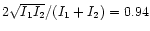
Analysis of the fringe tracker data shows that the experimental visibility Gvaries between 7 and 30 .
Figure 2 and Table 1
show that for r0 ranging between 10 and 16 cm at 0.5 m, G should be
of the order of
.
Figure 2 and Table 1
show that for r0 ranging between 10 and 16 cm at 0.5 m, G should be
of the order of  and
and  respectively. Since G is very sensitive to
static aberrations, the discrepancy between theoretical estimations and
experimental values is likely due to telescope focusing errors. Another
contribution is the scintillation effect. The R2 experimental values in the
scientific instrument span between 55 and 70 (Robbe 1996). These
results are consistent with the estimation of Table 1, also
taking into account the contribution of telescope focusing errors.
respectively. Since G is very sensitive to
static aberrations, the discrepancy between theoretical estimations and
experimental values is likely due to telescope focusing errors. Another
contribution is the scintillation effect. The R2 experimental values in the
scientific instrument span between 55 and 70 (Robbe 1996). These
results are consistent with the estimation of Table 1, also
taking into account the contribution of telescope focusing errors.
5 Fringe detection and tracking
The SIMONE demodulation algorithm (Sect. 3.2) was first tested in
the laboratory. Figure 3 shows a typical interferogram in bad
observing conditions (
 ). This interferogram is limited by photon
noise: there are about N=1400 photoevents per 3.5 ms sampling time.
Figure 3 also shows fringes outside the main lobe of the
interferogram. This is due to the significant amount of chromatism before
inserting the spectral filter in the fringe sensor
(
). This interferogram is limited by photon
noise: there are about N=1400 photoevents per 3.5 ms sampling time.
Figure 3 also shows fringes outside the main lobe of the
interferogram. This is due to the significant amount of chromatism before
inserting the spectral filter in the fringe sensor
(
 in Fig. 3).
![\begin{figure}
\par\includegraphics[width=8.8cm,clip]{ds1678F3.eps} %
\includegraphics[width=8.8cm,clip]{ds1678F4.eps}\end{figure}](/articles/aa/full/2001/02/aads1678/Timg88.gif) |
Figure 3:
Interferogram obtained from the detected intensity (top) and unbiased
squared visibility (bottom) versus OPD scan, in the laboratory, with
representative observingconditions (
,
392000 photoevents/s) |
| Open with DEXTER |
With the cophasing phase estimator, OPD correction was validated: a 90 Hz
open-loop bandwidth at 0 dB was achieved with a 500 Hz modulation, in
agreement with the loop simulation at high SNR. To reduce photon noise on the
sky for visibility measurements, the modulation frequency was reduced to
280 Hz (Eq. (4)). In the conditions of Fig. 3,
the servo-loop was automatically closed after fringe detection and was very
stable at a 40 Hz open-loop bandwidth. No fringe jumps were observed. But in
the laboratory no turbulence was simulated.
Visibility estimation was also validated. The visibility squared profile is
plotted with M=25 in Fig. 3. The coherence area is clearly
detected. The secondary peaks are due to the fringes in the secondary lobe of
the interferogram. Negative values of the V2 estimator may be surprising.
This is, however, required for an unbiased estimator to have a null
expectation outside the coherence area. V2 variance is about
 out of the coherence area, in agreement with Eq. (4).
The MAXSIM algorithm was also tested. The MAXSIM phase estimation for
cophasing performs as well as with SIMONE. The coherencing estimator worked
successfully with high visibility ( 30%). But by varying the fringe
visibility, the coherencing signal turned out to be very noisy for small
visibility levels since only a small portion of the envelope is scanned. It
would require averaging the coherencing signal over a few seconds to achieve a
sufficient SNR, but such a method was not tested.
30%). But by varying the fringe
visibility, the coherencing signal turned out to be very noisy for small
visibility levels since only a small portion of the envelope is scanned. It
would require averaging the coherencing signal over a few seconds to achieve a
sufficient SNR, but such a method was not tested.
![\begin{figure}
\par\includegraphics[width=8.5cm,clip]{ds1678F5.eps}\end{figure}](/articles/aa/full/2001/02/aads1678/Timg91.gif) |
Figure 4:
Typical visibility squared profiles obtained on 23 October 1995,
19:45 UT ( Cyg, solid) and on 24 October, 00:27 UT ( Cyg, solid) and on 24 October, 00:27 UT ( Per,
dotted) Per,
dotted) |
| Open with DEXTER |
Observations presented in this paper were made on the nights 7, 8, 21 and 23
October 1995 using the stars: Cyg (
 ),
Per (
),
Per (
 ),
),  Per (
Per (
 )
and
Cyg (
)
and
Cyg (
 ). Although the I2T baseline extends up to
140 m, all the measurements were made at a 15 m baseline to eliminate
misalignment problems due to the displacement of the pupil conjugation optics
(Robbe et al. 1994). Since the diameter of the collimated beams emerging
from the telescopes (11 mm) and the free atmosphere path (around 7 meters) are
small, the turbulence effects induced by the beam horizontal propagation from
the telescopes to the central laboratory are small.
). Although the I2T baseline extends up to
140 m, all the measurements were made at a 15 m baseline to eliminate
misalignment problems due to the displacement of the pupil conjugation optics
(Robbe et al. 1994). Since the diameter of the collimated beams emerging
from the telescopes (11 mm) and the free atmosphere path (around 7 meters) are
small, the turbulence effects induced by the beam horizontal propagation from
the telescopes to the central laboratory are small.
Glass plates were installed between the telescopes and the beam combining
table to compensate for longitudinal chromatism. The optimal thickness of the
glass plates was calculated in order to reduce the standard deviation of the
optical phase difference in the red spectral bandwidth
(Sorrente et al. 1994), and thus maximizing the measured fringe visibility
in the fringe sensor.
Fringe visibility and OPD were recorded with a 280 Hz sampling
frequency and the length of the data acquisition buffer typically corresponds
to 3 mn.
The first step is to detect the coherence area. Two stellar visibility
profiles, similar to that of Fig. 3, are shown in
Fig. 4 (
 ). The two
stars are unresolved for the baseline used. The maximum visibility for
Per, observed later in the night (00:27 UT), is higher than for
Cyg (19:45 UT). The turbulence strength decreased during the night
since the coherence time t0 (see Eq. (C.3)) was of the order of
5 ms in the beginning of the night and reached 10 ms in the middle of the
night. Since the goal of the fringe tracker is not to provide precise
visibility measurements, we did not investigate calibration of the measured
visibilities. Performance of the fringe detection is primarily driven by
off-fringe visibility fluctuations. One can notice this level in
Fig. 4: for Cyg, the secondary peaks are due to
noise and not to chromatism (like in Fig. 3) because of the use
of a spectral filter. The standard deviation of the measured visibility G2is
). The two
stars are unresolved for the baseline used. The maximum visibility for
Per, observed later in the night (00:27 UT), is higher than for
Cyg (19:45 UT). The turbulence strength decreased during the night
since the coherence time t0 (see Eq. (C.3)) was of the order of
5 ms in the beginning of the night and reached 10 ms in the middle of the
night. Since the goal of the fringe tracker is not to provide precise
visibility measurements, we did not investigate calibration of the measured
visibilities. Performance of the fringe detection is primarily driven by
off-fringe visibility fluctuations. One can notice this level in
Fig. 4: for Cyg, the secondary peaks are due to
noise and not to chromatism (like in Fig. 3) because of the use
of a spectral filter. The standard deviation of the measured visibility G2is
 ,
whereas the theoretical value is from
Eq. (4)
,
whereas the theoretical value is from
Eq. (4)
 (
(
 photoevents per modulation period and M=280 averaged periods).
For Per,
photoevents per modulation period and M=280 averaged periods).
For Per,
 whereas
 (
(
 and M=1440).
This shows that visibility noise is much higher than expected; we think this
results from scintillation effects (Sect. 3.1). Since this effect
has been understood lately, no dedicated measurement was made. But it may
a posteriori explain why, in similar photometric conditions, the off-fringe
mean visibility level reached 14% on 28 September 1995 whereas the maximum
off-fringe visibility during the other nights in October was a few percent.
Scintillation could have been reduced without increasing photon noise
(Eq. (4)) by multiplying the modulation frequency by an
integer factor p and extracting the phase after averaging, in intensity, psuccessive periods.
and M=1440).
This shows that visibility noise is much higher than expected; we think this
results from scintillation effects (Sect. 3.1). Since this effect
has been understood lately, no dedicated measurement was made. But it may
a posteriori explain why, in similar photometric conditions, the off-fringe
mean visibility level reached 14% on 28 September 1995 whereas the maximum
off-fringe visibility during the other nights in October was a few percent.
Scintillation could have been reduced without increasing photon noise
(Eq. (4)) by multiplying the modulation frequency by an
integer factor p and extracting the phase after averaging, in intensity, psuccessive periods.
The automatic detection algorithm performed well. In routine operation, good
knowledge of the instrument allowed considerable reduction of search time and
thus false alerts. The smallest detected visibility during the observations
was a few percent, but no dedicated measurement for ultimate sensitivity
determination was done.
5.4 Tracking performance
In the cophasing mode, MAXSIM and SIMONE have similar behaviour on the sky.
Unfortunately, it turned out during the few tests we made that the coherencing
mode of MAXSIM did not achieve the required performance because the visibility
in the experiment was too low (Sect. 4). This algorithm was thus
not characterized. All the data of this paper were collected with the SIMONE
algorithm.
In closed-loop, the 3 mn records are characterized by sequences where the
fringe tracker loses and recovers the coherence area after a few fringe jumps.
Because in the laboratory the loop was perfectly stable with a similar
light level without turbulence, the fringe jumps are due to the large
amplitude of the turbulent OPD fluctuations ( 10 m rms
from Eq. (C.1) for B=15 m, r0=10 cm and L0=40 m). Locked
sequences typically last 20 s from a fringe recovery to the next loss. However,
we stress that after fringe detection, the fringe tracker was able to operate
for more than one hour on the same star, in spite of the partial losses of the
coherence area which occur.
10 m rms
from Eq. (C.1) for B=15 m, r0=10 cm and L0=40 m). Locked
sequences typically last 20 s from a fringe recovery to the next loss. However,
we stress that after fringe detection, the fringe tracker was able to operate
for more than one hour on the same star, in spite of the partial losses of the
coherence area which occur.
In order to determine the performance of the servo and to estimate the
turbulence parameters from the recorded data, we only extract data sets where
the fringe tracker is locked on the fringes and where the visibility remains
quasi stable ( % rms), i.e. without fringe jumps. This is a very
restrictive selection. Such data sets last typically 10 s, but some
reach 20 s. In such conditions, only a few sets of measurements give
information at very low temporal frequency. Figure 5 illustrates
the fringe tracker operation for a visibility of 19.
The recorded signals
y(t), the PZT actuator position, and e'(t), the error signal, are plotted.
They approximate the turbulent OPD and the residual OPD error respectively
(Appendix A). A significant amount of OPD fluctuation is removed, while
the visibility remains quasi constant, showing that the fringe tracker is well
locked. The small visibility fluctuations can be attributed to photon noise,
seeing variations (Baldwin et al. 1994) and the effect of scintillation. The
reduction of the OPD fluctuations is of the order of 30 in terms of standard
deviation in Fig. 5. All the low frequencies are well filtered
out.
% rms), i.e. without fringe jumps. This is a very
restrictive selection. Such data sets last typically 10 s, but some
reach 20 s. In such conditions, only a few sets of measurements give
information at very low temporal frequency. Figure 5 illustrates
the fringe tracker operation for a visibility of 19.
The recorded signals
y(t), the PZT actuator position, and e'(t), the error signal, are plotted.
They approximate the turbulent OPD and the residual OPD error respectively
(Appendix A). A significant amount of OPD fluctuation is removed, while
the visibility remains quasi constant, showing that the fringe tracker is well
locked. The small visibility fluctuations can be attributed to photon noise,
seeing variations (Baldwin et al. 1994) and the effect of scintillation. The
reduction of the OPD fluctuations is of the order of 30 in terms of standard
deviation in Fig. 5. All the low frequencies are well filtered
out.
Figure 6a shows a power spectrum of the turbulent OPD, as
approximated by the PZT actuator position y(t), measured over 25 s.
Figure 6b shows the corresponding power spectrum of the error signal
e'(t). This spectrum is flat at high frequency because of photon noise. The
noise level is given by the horizontal line. The achieved accuracy is
0.1 m for a turbulence characterized by t0=12.4 ms at
0.85 m and 150500 photoevents/s. The open loop transfer function
|G(f)|2, plotted in Fig. 6c, is calculated as the power spectrum
ratio of y(t) by e'(t) (Appendix A). The experimental transfer
function is very close to the f-2 theoretical law of an integral
corrector as a feedback controller. In Fig. 6c the open-loop
bandwidth at 0 dB
 is 20 Hz.
![\begin{figure}
\par\includegraphics[width=8.8cm,clip]{ds1678F6.eps}\end{figure}](/articles/aa/full/2001/02/aads1678/Timg106.gif) |
Figure 5:
Visibility versus time when the fringe tracker is active (top),
 %. Simultaneously measured turbulent OPD, y(t), and residual
OPD, e'(t), versus time (bottom). Rms accuracy of the servo:
0.081
for a turbulent OPD of 2.6
rms. Curves obtained on 21 October 1995, 01:01 UT, star: Per %. Simultaneously measured turbulent OPD, y(t), and residual
OPD, e'(t), versus time (bottom). Rms accuracy of the servo:
0.081
for a turbulent OPD of 2.6
rms. Curves obtained on 21 October 1995, 01:01 UT, star: Per |
| Open with DEXTER |
![\begin{figure}
\par\includegraphics[width=8.8cm,clip]{ds1678F7.eps} %
\includegr...
...ip]{ds1678F8.eps} %
\includegraphics[width=8.8cm,clip]{ds1678F9.eps}\end{figure}](/articles/aa/full/2001/02/aads1678/Timg107.gif) |
Figure 6:
Power spectrum densities of a) the PZT actuator position y(t), b)
the error signal e'(t), c) open loop transfer function |G(f)|2 of the
fringe tracker. Measured on 7 October 1995, 19:05 UT, star:
Cyg. Curves fitted by: a) f-2/3 and f-8/3 laws, b) level
of white noise, c) f-2 law |
| Open with DEXTER |
![\begin{figure}
\par\includegraphics[width=8.8cm,clip]{ds1678F10.eps}\end{figure}](/articles/aa/full/2001/02/aads1678/Timg108.gif) |
Figure 7:
Accuracy,
 (top), and rms noise
 (bottom),versus fringe visibility in log-log scales
for four runs detailed in Table 2. A line with slope of -1 is
shown
(bottom),versus fringe visibility in log-log scales
for four runs detailed in Table 2. A line with slope of -1 is
shown |
| Open with DEXTER |
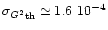
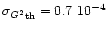
The performance of the fringe tracker is measured by the standard deviation
of the true OPD residual error e(t).
 is derived
from the variances
is derived
from the variances
 of the error signal measured by the fringe
sensor and
of the error signal measured by the fringe
sensor and
 of the noise estimated at high frequency on the
error signal spectrum (Appendix A). Figure 7 presents the
measurements of the rms residual error
and the rms noise
(photon noise) versus the measured visibility. As seeing
conditions may rapidly change during observation, we plot
and
measured on fringe-locked sequences with various visibility
levels for four records of 3 mn. The conditions of the measurements are
summarized in Table 2. For visibilities spanning between 7 and
24%, an average OPD accuracy (
)
of 85 nm (
of the noise estimated at high frequency on the
error signal spectrum (Appendix A). Figure 7 presents the
measurements of the rms residual error
and the rms noise
(photon noise) versus the measured visibility. As seeing
conditions may rapidly change during observation, we plot
and
measured on fringe-locked sequences with various visibility
levels for four records of 3 mn. The conditions of the measurements are
summarized in Table 2. For visibilities spanning between 7 and
24%, an average OPD accuracy (
)
of 85 nm (
 at
0.85 m) is achieved. From Fig. 7 and Table 2
several comments can be made:
at
0.85 m) is achieved. From Fig. 7 and Table 2
several comments can be made:
- As given in Eq. (3),
follows the
V-1 law. The dependence in N-1/2 is also roughly verified;
-
does not depend on the visibility V. Note that
is the sum of two contributions: the turbulence uncompensated
residual OPD and the part of the photon noise propagated through the
servo-loop (Appendix A). Only the second contribution depends on the
visibility (as
). For the considered light levels, the accuracy
is dominated by the turbulence residuals. This is due to the
servo-loop bandwidth being too low, i.e. the loop-gain which was crudely
optimized by the observer was too low (Sect. 2.2). Indeed
in Fig. 7 and Table 2, the comparison of Curves band c on one hand and of Curves a and d on the other hand shows the
performance dependence on the coherence time and the bandwidth, respectively.
Moreover, when the number of photoevents decreases by a factor of 2 to 3, no
clear evidence of a loss of accuracy is shown.
No tests of limiting magnitude have been performed. Nevertheless, fringes have
been stabilized on a 2.48 magnitude star (Cyg) with an accuracy of
the order of
at 0.85 m for t0=8 ms, an overall optical
throughput estimated to be of the order of 0.8% and a 80 nm spectral
bandwidth. Using Eqs. (A.1) and (A.3) and the measured
observing conditions, we checked by simulation (as in Sect. 4.2)
that the experimental performance ()
was close to the theoretical
one. If all the coatings of the optical surfaces were optimized, the
throughput would have reached 10% and the
accuracy would have
been achieved on a 5 magnitude star in the I2T-ASSI configuration for the same
turbulence conditions.
Using the same simulation, it is possible to evaluate the performance of the
fringe tracker presented here for an interferometer working with 8 m apertures
partially corrected by adaptive optics (Rousset et al. 1991) and a 40 m
baseline. The fringe tracking technique working in H band would lead to a
100 nm OPD accuracy in the following conditions: mH=15 (80000
photoevents/s), 15% fringe visibility, r0=14 cm at 0.5 m,
v=10 ms-1, L0=40 m and 50 Hz bandwidth. For a scientific observation
made at 2.2 m, the tracking performance is then of the order of
/22. We stress that the limiting magnitude depends on the specified
OPD accuracy and on the seeing conditions.
Table 2:
Conditions of measurements of Fig. 7. The flux
corresponds to the number of photoevents per second.
is
the open-loop bandwidth at 0 dB. Coherence time t0 given at
0.85 m (Eq. (C.2))
| Curve |
a |
b |
c |
d |
| Date (1995) |
10/7 |
10/23 |
10/21 |
10/23 |
| Star |
Cyg |
Cyg |
Per |
Per |
| N (photoevents/s) |
150500 |
127200 |
100700 |
58600 |
|
(Hz) |
20 |
40 |
40 |
50 |
| t0 (ms) |
12.3 |
13.9 |
4.5 |
8.1 |
6 Seeing characterization
6.1 Fringe tracker measurements
The fringe tracker bandwidth is sufficiently large to check the agreement of
the data with the Kolmogorov model (see Appendix C) at frequencies lower
than 20 Hz, as illustrated in Fig. 6a. A fit with -2/3 and
-8/3 power laws is superimposed.
We determined the high frequency slope of 30 power spectra of y(t). They
have been processed as follows: an autoregressive filter (Makhoul 1975) is
first estimated from the temporal data. Then, a polynomial fit of the filter
is made. The slope of the high frequency part of the spectrum is determined at
the inflection point of the polynomial fit. The main advantage of this method
is that the slope at the inflection point is less corrupted than at other
points of the spectrum by the low frequency behavior and by the noise
appearing at very high frequency.
The average value is -7.84/3 with a dispersion of  .
We conclude
that the -8/3 regime predicted by the Kolmogorov model (Appendix C) is
in good agreement with our measurements. From all our data, no evidence of a
-17/3 regime was observed for
f > 0.3v/D (10 Hz for
v=10 ms-1) although the bandwidth of the servo can be as large as
50 Hz in some records. We think this results from the aliasing of the
high order phase distorsions in the OPD measurement by temporal modulation.
Indeed, the high order phase distorsions have temporal frequency spectra
spanning higher frequencies than the OPD one (Conan et al. 1995).
.
We conclude
that the -8/3 regime predicted by the Kolmogorov model (Appendix C) is
in good agreement with our measurements. From all our data, no evidence of a
-17/3 regime was observed for
f > 0.3v/D (10 Hz for
v=10 ms-1) although the bandwidth of the servo can be as large as
50 Hz in some records. We think this results from the aliasing of the
high order phase distorsions in the OPD measurement by temporal modulation.
Indeed, the high order phase distorsions have temporal frequency spectra
spanning higher frequencies than the OPD one (Conan et al. 1995).
According to Eq. (C.2), t0 can be calculated from the fit of the high
frequency part of the fringe motion spectra with the autoregressive filter
technique. Mean values of t0 corresponding to four nights of observations
are quoted in Table 3. The coherence time was typically equal to
9 ms in the
0.81-0.89
spectral range of the
fringe sensor.
6.2 Star tracker measurements
According to Appendix C, r0, v and L0 can be estimated from the
variance and the power spectrum of the angle of arrival. r0 and vestimations have already been published in the first paper (Robbe et al. 1997).
Autoregressive filters are used to fit angle of arrival spectra in order to
determine the seeing parameters. Figure 8 shows a power spectrum
obtained from a 3 mn long data record of the x axis of the south tip-tilt
mirror. The telescope drift is removed from the data after checking that no
mirror actuator desaturation occurs during the record. The fitting of the
spectrum of Fig. 8 with an autoregressive filter shows
f-2.4/3 and f-10/3 laws close to the theory
(Fig. C.1). For all the data sets of the four nights the
measured average slopes are
 at low frequency and
 at high frequency. This confirms the evidence of the
Kolmogorov behavior for frequency higher than 0.2 Hz. However, the most
interesting point is at very low frequency: the clear deviation from the
Kolmogorov model, peculiar to a finite outer scale. This saturation effect was
observed on a large number of angle of arrival power spectra during the
observations of October 1995. We checked that the flattening effect was not
due to the removal of the telescope drift, simulating a temporal sequence of
angle of arrival obeying the Kolmogorov model, and removing the drift due to
the turbulence itself.
at high frequency. This confirms the evidence of the
Kolmogorov behavior for frequency higher than 0.2 Hz. However, the most
interesting point is at very low frequency: the clear deviation from the
Kolmogorov model, peculiar to a finite outer scale. This saturation effect was
observed on a large number of angle of arrival power spectra during the
observations of October 1995. We checked that the flattening effect was not
due to the removal of the telescope drift, simulating a temporal sequence of
angle of arrival obeying the Kolmogorov model, and removing the drift due to
the turbulence itself.
A L0-independent estimation of r0 requires an extrapolation of the
-2/3 Kolmogorov behavior at very low frequency in order to compensate for
the effects of the saturation due to L0 and in addition for the finite
duration of the record. The second parameter deduced from the angle of arrival
is the average wind speed, v, estimated from the knee frequency f2(Appendix C). As shown in Fig. 8, the -2/3 and the
-11/3 regimes can be clearly distinguished. From r0 and v we derive
t0 through Eq. (C.3). The estimated values of these parameters
are gathered in Table 3. Estimations of t0 deduced from the
fringe tracker data and the angle of arrival data are in agreement. Note that
the data recordings on the star tracker and the fringe tracker were generally
not simultaneous, but not too much delayed.
![\begin{figure}
\par\includegraphics[width=8.5cm,clip]{ds1678F11.eps}\end{figure}](/articles/aa/full/2001/02/aads1678/Timg132.gif) |
Figure 8:
Power spectrum of the angle of arrival measured on the south x axis
of the star tracker and fitted by an autoregressive filter. Measured on 8
october 1995, 19:19 UT, star: Cyg. Horizontal line: level of white
noise |
| Open with DEXTER |
6.3 Outer scale estimation
The analysis of the angle of arrival spectra obtained in October
1995 leads to a value of the first knee frequency, f0, varying between 0.1
and 0.3 Hz. L0 is derived from f0 using v estimated on the same
spectrum from f2. L0 typically ranges from 20 to 50 m during the
observations. The average value is 40 m. Such a method presents systematic
errors in the estimation of the outer scale since the determination of the
first knee frequency, f0, depends on the obtained fit of the -2/3 regime.
Another way to estimate the outer scale from the angle of arrival data is
to compare the experimental variance to the theoretical von-Karman variance
(Eq. (C.4)). The outer scale was calculated using the instantaneous
value of r0 derived in Sect. 6.2. Values of L0 from 1 to
120 m (mean value of 25 m) are found. The dispersion of the measurements is
more important here: obviously L0 values are very sensitive to r0estimation. An error of 5% in r0 leads to an error of 50% in L0. Small
values of L0 are not consistent with the observed shape of the power
spectra, since an outer scale of a few meters would lead to f0 of the order
of 1 Hz. Clearly, this was never observed.
L0 may also be estimated by comparing the theoretical von-Karman variance
(Eq. (C.1)) to the experimental variance of the fringe motion, also
taking into account the effect of the finite duration of the measurements.
r0 is deduced from t0 obtained from the OPD spectrum and vcorresponding to the closest record of angle of arrival. From the OPD data,
L0 typically ranges between 30 m and 120 m, with an average value of 50 m.
These results are consistent with the estimations derived from the angle of
arrival data. Furthermore, as for the case of the angle of arrival spectra,
the observed knee frequency of the OPD spectra is always close to 0.2 Hz.
Finally, the estimates of the outer scale typically range between 20 and
120 m. Values smaller than 10 m are not compatible with our observations.
We have described the fringe tracker system of the ASSI table developed to
compensate in real-time the I2T interferometer for the turbulent OPD. The PZT
delay line is controlled by a fringe sensor based on a temporal modulation and
equipped with a photon-counting APD. The free parameters of the sensor, i.e.
the modulation function, the number of buckets and the demodulation algorithm
have been optimized for best performance. Unlike similar systems based on
triangle modulation and the DFT algorithm, a sinusoidal modulation is used.
Visibility estimation or closed-loop phase measurements can be optimized by
the choice of the modulation amplitude. This new algorithm, so-called SIMONE,
has been tested and validated on the sky for fringe detection and cophasing.
It is based on a sinusoidal OPD modulation of amplitude
 and has
performance similar to that of the ABCD algorithm. A large number of buckets
(16) ensures minimum visibility loss without any extra cost. The modulation
frequency is 280 Hz. The bandwidth is adjusted by a numerical gain according
to the observing conditions. In the reported experiments the bandwidth ranges
between 20 and 50 Hz.
and has
performance similar to that of the ABCD algorithm. A large number of buckets
(16) ensures minimum visibility loss without any extra cost. The modulation
frequency is 280 Hz. The bandwidth is adjusted by a numerical gain according
to the observing conditions. In the reported experiments the bandwidth ranges
between 20 and 50 Hz.
The fringe tracker (SIMONE algorithm) achieves a typical OPD accuracy of
/10 at 0.85 m for a visibility ranging between 7 and 24%, a
coherence time t0 around 9 ms and a 2 magnitude star. With optimized
optical throughput, this performance would have been achieved on a 5 magnitude
star. High temporal bandwidth (around 50 Hz in open-loop) is required to
obtain good performance for bright stars. For low bandwidth or small r0,
OPD residuals are such that the cophasing algorithm suffers from fringe jumps.
Fringe-locked sequences typically last 20 s. However, the fringe tracker
operation can last more than one hour without fatal loss of the coherence
area. It was not possible to successfully implement the coherencing algorithm
because the visibility on the sky was too low. Sometimes, scintillation was
found to severely limit the system. The modulation frequency should have been
higher, taking advantage of the sinusoidal modulation.
Visibility losses are estimated in the ASSI-I2T interferometer. They are
mainly due to the static aberrations of the optical train and the wavefront
fluctuations due to the turbulence. For the fringe sensor, the visibility is
lower than 24% for r0=10 cm at 0.5 m. This estimation is in good
agreement with the measured visibilities. For the scientific instrument, the
visibility is lower than 70%.
Turbulence parameters are characterized for the evaluation of the observing
conditions. The temporal power spectra of the fringe motion are well modeled
by the Kolmogorov statistics at high frequency since an average slope of
-7.8/3 has been measured for the -8/3 theoretical prediction.
This expected
behavior allows us to determine the coherence time, t0. An average
coherence time of the order of 9 ms at 0.85 m was estimated during the
observations of October 1995. The agreement between the estimations of t0derived from the data of the star and fringe trackers underlines the
reliability of the Kolmogorov model at very different scales in the inertial
range: 0.26 m for the star trackers and 15 m for the fringe tracker. Our
observations corresponds to average seeing conditions with r0 ranging
between 8 and 18 cm at 0.5 m.
The star tracker data show that the angle of arrival spectra depart at very
low frequency from the theoretical prediction based on the pure Kolmogorov
model. Analysis of these data leads to an average outer scale of the order of
40 m with a range of variation between 20 and 120 m. This estimation was
confirmed by the analysis of the fringe tracker data.
Lessons learned from ASSI experiment recently have been used in the
design of a new fringe tracker for the VLTI (Cassaing 2000). Since the
fringe tracker generally differs from the scientific instrument, algorithms
optimized for fringe tracking should be used instead of the triangle
modulation of amplitude
optimized for visibility measurements.
Moreover, spatial modulation avoids cross-talk present in temporal modulation
between OPD measurement, turbulent intensity fluctuation induced by
scintillation, high order wavefront distorsions and high temporal frequencies
of the residual OPD. Finally, coherencing should be performed by dispersion,
as in most other interferometers (Armstrong et al. 1998;
Colavita et al. 1999).
Acknowledgements
The authors wish to thank the anonymous referee for his or her helpful and
numerous comments, C. Dessenne for her fruitful advice in the data processing,
G. Merlin for his support during the observations, C. Coudrain and L.
Ménager for their participation in the fringe tracker development. This
study was funded by the Direction des Recherches, Études et Techniques of
the French Defense Ministry.
The block diagram of the fringe tracker is illustrated in
Fig. A.1. The residual OPD error, e(t), seen by the scientific
instrument and the fringe sensor, is the difference between the incoming OPD
due to turbulence a(t) and the PZT actuator position y(t). e(t)represents the accuracy of the servo-loop. The error signal e'(t) as
measured by the fringe sensor is corrupted by white noise n(t).
Let's call G(f) the transfer function of the fringe tracker (including
sensor, computer and delay line), where f is the temporal frequency.
According to Fig. A.1, the following relations hold, denoting with
 the spectrum of the temporal variables:
The noise n is uncorrelated from the residual error e,
 (Dessenne et al. 1998), thus it is
possible to derive the actual performance of the system
since
can be estimated from the power spectrum of e' with an
autoregressive filter. Equation (A.1) shows that
(Dessenne et al. 1998), thus it is
possible to derive the actual performance of the system
since
can be estimated from the power spectrum of e' with an
autoregressive filter. Equation (A.1) shows that
 is
composed of two terms related to a and n. Since at high frequency (G(f)
is
composed of two terms related to a and n. Since at high frequency (G(f) 1) a has a fast decreasing power spectrum (see Appendix C), then
tends to the white spectrum of the noise. Hence, the noise
level can be estimated.
1) a has a fast decreasing power spectrum (see Appendix C), then
tends to the white spectrum of the noise. Hence, the noise
level can be estimated.
![\begin{figure}
\par\includegraphics[width=8.8cm,clip]{ds1678F12.eps}
\end{figure}](/articles/aa/full/2001/02/aads1678/Timg144.gif) |
Figure A.1:
Block diagram of the fringe tracker servo |
Since
 for
for
 ,
,
 the closed-loop
bandwidth,
the closed-loop
bandwidth,
 is representative of the turbulence fluctuations
assuming that
is representative of the turbulence fluctuations
assuming that
 in this domain (see
Eq. (A.3)). Hence, the spatial and temporal characteristics of the
turbulence can be directly deduced from the signal
.
in this domain (see
Eq. (A.3)). Hence, the spatial and temporal characteristics of the
turbulence can be directly deduced from the signal
.
Finally, Eq. (A.2) shows that it is possible to adjust the gain in
G(f) in order to minimize the residual error, taking into account the
respective levels of turbulence and noise, i.e. the observing conditions.
The factors other than optical aberrations which reduce the fringe visibility
are:
- The field rotation attenuation factor, which depends on the star
declination (Koechlin 1985). Since we chose stars close to the zenith, this
factor around the transit (
1 hour) is not important: typically, 0.97;
- Differential polarization effects. They may appear when each beam does
not encounter the same sequence of reflections (Traub 1988). Measurements
of the Jones matrices of the two arms revealed an important chromatic
differential effect. A vertical polarizer and a 80 nm filter centered on
0.85 m, which corresponds to a 9 m coherence length, were
placed before the APD. They allow the elimination of this problem, since the
north and south Jones matrices are diagonal. The main drawback is that half of
the light is rejected;
- Differential chromatism (Lacasse & Traub 1988), including longitudinal
dispersion and atmospheric refraction. Differential diffraction and residual
longitudinal chromatism after the glass plates were simulated. Their effect on
fringe visibility is negligible since the baseline (around 15 m) and the
zenith angle are small. The chromatism, introduced by the refractive optics
of the ASSI table, is also reduced by the use of the spectral filter;
- Differential intensity. Intensities in the north and south beams differ
by a factor of 2 because of different throughputs. The attenuation factor is
therefore
 .
.
In stellar interferometry, when  ,
the variance of the turbulent phase
of the interferogram can be approximated by
,
the variance of the turbulent phase
of the interferogram can be approximated by
 with:
with:
![\begin{displaymath}D_\varphi(\V{B})=3.69\left(\frac{r_0}{L_0}\right)^{-\frac53}
...
...a(\frac{11}6)}K_{\frac56}\!\!\left(\frac{B}{L_0}\right)\right]
\end{displaymath}](/articles/aa/full/2001/02/aads1678/img153.gif) |
(C.1) |
where
 is the modified Bessel function of order 5/6.
 is the phase structure function computed by Valley
(1979) for a modified Kolmogorov spectrum, taking into account the
effect of a finite outer scale L0 (von-Karman spectrum). Therefore, the
measurement of
is the phase structure function computed by Valley
(1979) for a modified Kolmogorov spectrum, taking into account the
effect of a finite outer scale L0 (von-Karman spectrum). Therefore, the
measurement of
 by the fringe sensor can be used to estimate
the two turbulent parameters r0 and L0, for instance by varying the
baseline (Mariotti & Di Benedetto 1984).
by the fringe sensor can be used to estimate
the two turbulent parameters r0 and L0, for instance by varying the
baseline (Mariotti & Di Benedetto 1984).
![\begin{figure}
\par\includegraphics[width=8.5cm,clip]{ds1678F13.eps}\end{figure}](/articles/aa/full/2001/02/aads1678/Timg157.gif) |
Figure C.1:
Theoretical power spectra of: a) fringe motion (in
 Hz-1) and b) angle of arrival (in arcsec2 Hz-1) for a pure
Kolmogorov model (dashed line), for a von-Karman model with L0=40 m
(dotted line) and L0=400 m (solid line). r0=10 cm at 0.5 m,
B=15 m, D=0.26 m and v=10 Hz-1) and b) angle of arrival (in arcsec2 Hz-1) for a pure
Kolmogorov model (dashed line), for a von-Karman model with L0=40 m
(dotted line) and L0=400 m (solid line). r0=10 cm at 0.5 m,
B=15 m, D=0.26 m and v=10
 .
The knee frequencies f0(for L0=400 m), f1, f2 and the exponents of the power laws are
given .
The knee frequencies f0(for L0=400 m), f1, f2 and the exponents of the power laws are
given |
Considering the von-Karman model, it can be shown that the theoretical
temporal power spectrum of the OPD fluctuations (Buscher et al. 1995;
Conan et al. 1995)
can be divided into different cases as plotted in Fig. C.1:
- At very low frequencies,
f<f0=v/L0 where v is the average wind
speed, the spectrum flattens to a f0 power law as the result of the finite
outer scale;
- At low frequency,
f0<f<f1=0.2v/B, the conventional Kolmogorov
f-2/3 law holds. We stress that for outer scales of the order of a few
tenth of meters, this regime is not observable in the spectrum
(
 );
);
- At high frequency,
f1<f<f2=0.3v/D, the spectrum shows the
conventional Kolmogorov f-8/3 law. In this case the phases on the two
telescopes are independent, the OPD power spectrum is twice the phase power
spectrum;
- At very high frequency, f2<f, the spectrum obeys a
f-17/3 law.
Following Buscher (1995), the coherence time t0 can be deduced
from the vertical position of the f-8/3 asymptote of the power spectrum
 ,
since:
,
since:
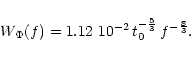 |
(C.2) |
The advantage of this method is that t0 estimation is not affected by the
value of L0. According to Taylor's hypothesis, t0 can also be deduced
from the knowledge of r0 and the average wind speed v by the relation
(Roddier et al. 1982):
 |
(C.3) |
The variance of the angle of arrival
on each telescope
 is directly linked to r0 and L0(Fante 1975; Ziad 1993):
As shown in Fig. C.1, the theoretical temporal power spectrum
of the angle of arrival tends also to a f-2/3 law at low frequency while
the high frequency component is characterized by a f-11/3 power law. These
regimes are separated by a knee frequency
f2=0.3v/D (Conan et al. 1995). As
for the case of the OPD, the power spectrum saturates at frequencies lower
than f0=v/L0 and a f0 behavior is also predicted for the von-Karman
model. Even for L0=40 m the f-2/3 regime is clearly observed in the
angle of arrival spectrum but not in the OPD spectrum.
- Armstrong,
J. T., Mozurkewich, D., Rickard, L. J., et al. 1998, ApJ, 496, 550
In the text
NASA ADS
-
Baldwin, J. E., Boysen, R. C., Cox, G. C., et al. 1994, in
(Breckinridge In the text
1994), 112
- Beckers,
J. M., Merkle, F. (ed.) 1991, ESO Proc. 39, High-Resolution Imaging by
Interferometry II
In the text
-
Bester, M., Danchi, W. C., Degiacomi, C. G., et al. 1992,
Astrophys. J., 357
In the text
-
Breckinridge, J. B. (ed.) 1994, Proc. SPIE 2200,
Amplitude and Intensity Spatial Interferometry II
In the text
-
Buscher, D. F., Armstrong, J. T., Hummel, C. A., et al. 1995,
Appl. Opt., 34(6), 1081
In the text
NASA ADS
-
Cassaing, F., Mugnier, L., Sorrente, B., et al. 1995,
Technical Report 4/4625 PY, ONERA
In the text
-
Cassaing, F., Mugnier, L., Sorrente, B., et al. 1996,
Technical Report 8/4625 PY, ONERA
In the text
-
Cassaing, F. 1997,
Ph.D. Thesis, Université Paris XI Orsay
In the text
-
Cassaing, F., Fleury, B., Coudrain, C., et al. 2000, in Proc. SPIE 4006,
Interferometry in optical astronomy
In the text
-
Colavita, M. M., Wallace, J. K., Hines, B. E., et al. 1999,
Astrophys. J., 510(1)
In the text
- Conan,
J.-M., & Rousset, G. 1995, in ESO Proc. 54, Topical Meeting on Adaptive Optics, 351
In the text
-
Conan, J.-M., Rousset, G., & Madec, P.-Y. 1995,
J. Opt. Soc. Am. A, 12(12), 1559
In the text
NASA ADS
-
Damé, L., Faucherre, M., Bourdet, G., et al. 1988,
in (Merkle In the text
1988), 1079
-
Davis, J., Lawson, P. R., Booth, A. J., et al.
1995,
Mon. Not. R. Astr. Soc., 273, L53
In the text
NASA ADS
-
Dessenne, C., Madec, P. Y., & Rousset, G. 1998,
Appl. Opt., 37(21), 4623
In the text
NASA ADS
-
Fante, R. 1975,
Proc. IEEE, 63(12), 1669
In the text
NASA ADS
-
Koechlin, L. 1985,
Ph.D. Thesis, Université de Nice
In the text
-
Koechlin, L., & Rabbia, Y. 1985,
A&A, 153, 91
In the text
NASA ADS
-
K
 chlin, L., Lawson, P. R., Mourard, et al. 1996, Appl. Opt., 35(16), 3002
In the text
chlin, L., Lawson, P. R., Mourard, et al. 1996, Appl. Opt., 35(16), 3002
In the text
-
Labeyrie, A. 1975,
ApJ, 196, L71
In the text
NASA ADS
-
Lacasse, M. G., & Traub, W. A. 1988,
in (Merkle In the text
1988), 959
-
Makhoul, J. 1975,
in Proc. IEEE, vol. 63, 561
In the text
-
Mariotti, J., & Di Benedetto, G. 1984,
in Very Large Telescopes, their Instrumentation and Programs,
vol. 79, 257, IAU, ed. M.-H. Ulrich, & K. Kjär
In the text
- Merkle, F.
(ed.) 1988, ESO Proc. 29, High-resolution imaging by interferometry
In the text
-
Mourard, D., Tallon-Bosc, I., Rigal, F., et al. 1994,
A&A, 288, 675
In the text
NASA ADS
-
Robbe, S. 1996,
Ph.D. Thesis, Université de Nice-Sophia Antipolis
In the text
-
Robbe, S., Sorrente, B., Cassaing, F., et al. 1997,
A&A, 125, 1
In the text
- Robbe, S.,
Sorrente, B., Cassaing, F., et al. 1994, in (Breckinridge In the text
1994), 222
-
Roddier 1981,
Progress in Optics, ed. E. Wolf, XIX, 281
In the text
-
Roddier, F., Gill, J. M., & Lund, G. 1982,
J. Optics (Paris), 13(5), 263
In the text
NASA ADS
-
Roddier, F., & Léna, P. 1984,
J. Optics (Paris), 15(4), 171
In the text
NASA ADS
-
Rousset, G., Madec, P. Y., & Rabaud, D. 1991,
in (Beckers In the text
1988), 1095
-
Shao, M., Colavita, M. M., Hines, B. E., et al. 1988,
A&A, 193, 357
In the text
NASA ADS
- Sorrente,
B., Cassaing, F., Beal, D., et al. 1991,
in (Beckers In the text
1988), 1133
-
Sorrente, B., Cassaing, F., & Rousset, G. 1994,
Technical Report 3/4625 PY, ONERA
In the text
-
Traub, W. A. 1988,
in (Merkle In the text
1988), 1029
-
Valley, G. C. 1979,
Appl. Opt., 18(7), 984
In the text
NASA ADS
-
Ziad, A. 1993,
Ph.D. Thesis, Université Nice-Sophia Antipolis
In the text
© ESO 2001
![\begin{figure}
\par\includegraphics[width=8cm,clip]{ds1678F2.eps}\end{figure}](/articles/aa/full/2001/02/aads1678/img80.gif)
![\begin{figure}
\par\includegraphics[width=8.8cm,clip]{ds1678F3.eps} %
\includegraphics[width=8.8cm,clip]{ds1678F4.eps}\end{figure}](/articles/aa/full/2001/02/aads1678/img88.gif)
![\begin{figure}
\par\includegraphics[width=8.5cm,clip]{ds1678F5.eps}\end{figure}](/articles/aa/full/2001/02/aads1678/img91.gif)
![\begin{figure}
\par\includegraphics[width=8.8cm,clip]{ds1678F6.eps}\end{figure}](/articles/aa/full/2001/02/aads1678/img106.gif)
![\begin{figure}
\par\includegraphics[width=8.8cm,clip]{ds1678F7.eps} %
\includegr...
...ip]{ds1678F8.eps} %
\includegraphics[width=8.8cm,clip]{ds1678F9.eps}\end{figure}](/articles/aa/full/2001/02/aads1678/img107.gif)
![\begin{figure}
\par\includegraphics[width=8.8cm,clip]{ds1678F10.eps}\end{figure}](/articles/aa/full/2001/02/aads1678/img108.gif)
![\begin{figure}
\par\includegraphics[width=8.5cm,clip]{ds1678F11.eps}\end{figure}](/articles/aa/full/2001/02/aads1678/img132.gif)
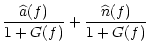
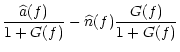
![$\displaystyle \big[\widehat{a}(f)+\widehat{n}(f)\big]\frac{G(f)}{1+G(f)}\cdot$](/articles/aa/full/2001/02/aads1678/img140.gif)
![\begin{figure}
\par\includegraphics[width=8.5cm,clip]{ds1678F13.eps}\end{figure}](/articles/aa/full/2001/02/aads1678/img157.gif)
![$\displaystyle -0.367\left(\frac{D}{L_0}\right)^\frac{10}{3}+...\bigg].$](/articles/aa/full/2001/02/aads1678/img166.gif)