2 Observations

2.1 IRAM 30-m observations and results

We have observed the $J=1\rightarrow 0$ and $J=2 \rightarrow 1$ lines of and with the IRAM 30-m telescope (Pico de Veleta, Spain) towards the GC molecular clouds given in Table 1.

   

Table 1: J2000 coordinates of the sources

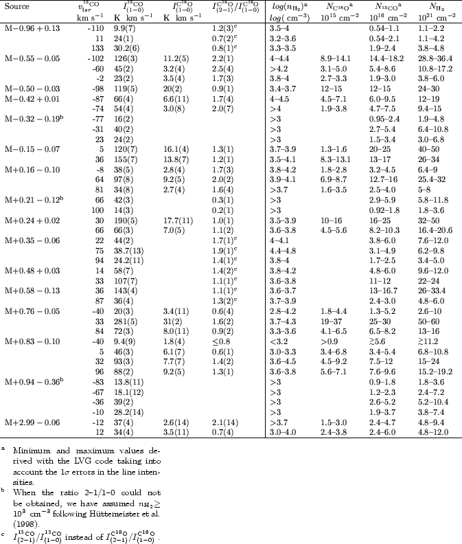
Source	RA	DEC	Complex
	h m s	$^\circ$ ' ''
M -0.96+0.13	17:42:48.3	-29:41:09.1	Sgr E
M -0.55-0.05	17:44:31.3	-29:25:44.6	Sgr C
M -0.50-0.03	17:44:32.4	-29:22:41.5	Sgr C
M -0.42+0.01	17:44:35.2	-29:17:05.4	Sgr C
M -0.32-0.19	17:45:35.8	-29:18:29.9	Sgr C
M -0.15-0.07	17:45:32.0	-29:06:02.2	Sgr A
M +0.16-0.10	17:46:24.9	-28:51:00.0	Arc
M +0.21-0.12	17:46:34.9	-28:49:00.0	Arc
M +0.24+0.02	17:46:07.9	-28:43:21.5	Dust Ridge
M +0.35-0.06	17:46:40.0	-28:40:00.0
M +0.48+0.03	17:46:39.9	-28:30:29.2	Dust Ridge
M +0.58-0.13	17:47:29.9	-28:30:30.0	Sgr B
M +0.76-0.05	17:47:36.8	-28:18:31.1	Sgr B
M +0.83-0.10	17:47:57.9	-28:16:48.5	Sgr B
M +0.94-0.36	17:49:13.2	-28:19:13.0	Sgr D
M +2.99-0.06	17:52:47.6	-26:24:25.3	Clump 2

This table also gives the pointing positions and the complexes where the clouds belong. Figure 1 shows the position of the sources overlayed on the large scale ( $1\rightarrow 0$) map of Dahmen et al. (1997).

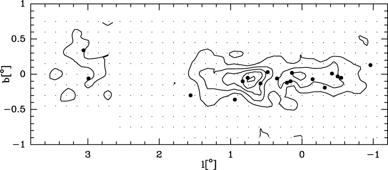Figure 1: The positions of all the sources of our sample (including the two clouds presented in Rodríguez-Fernández et al. 2000) overlayed in the (1-0) map by Dahmen et al. (1997)

The observations were carried out in May 1997, May 1998 and June 2000. The $J=1\rightarrow 0$ and $J=2 \rightarrow 1$ lines were observed simultaneously, with two $512\times 1$ MHz channel filter banks connected to two SIS receivers at 3 and 1.3 mm. The receivers were tuned to single side band mode. The image rejection, checked against standard calibration sources, was always larger than 10 dB. Typical system temperatures were $\sim \,$250 K for the $J=1\rightarrow 0$ lines and $\sim \,$400 K for the $J=2 \rightarrow 1$ lines. The velocity resolution obtained with this configuration was 2.7 and 1.4 kms^-1 at 3 and 1.3 mm respectively. The beam size of the telescope was 22'' for the $J=1\rightarrow 0$ lines and 11'' for the $J=2 \rightarrow 1$ line. Pointing and focus were monitored regularly. The pointing corrections were never larger than 3''. The spectra were taken in position switching with a fixed reference position at $(l,b)=(0\hbox{$.\!\!^\circ$ }65,~0\hbox{$.\!\!^\circ$ }2)$, which was selected from the map of Bally et al. (1987). Calibration of the data was made by observing hot and cold loads with known temperatures, and the line intensities were converted to main beam brightness temperatures, $T_{\rm MB}$, using main beam efficiencies of 0.68 and 0.41 for 3 and 1.3 mm respectively. The main beam efficiencies for the observations of June 2000 are 0.80 and 0.53 for 3 and 1.3 mm respectively.

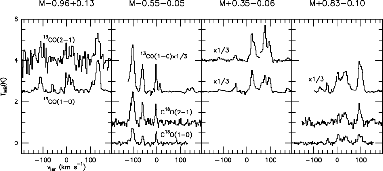
A sample of spectra is shown in Fig. 2. Most of the sources show CO emission in several velocity components with Gaussian profiles.

Figure 2:   and   spectra of four sources

However, in some clouds the different components are blended, giving rise to more complex profiles. The observed parameters derived from Gaussian fits are listed in Table 2.

  

Table 2: Observational parameters and LVG results for the CO data: Integrated intensities of the $J=1\rightarrow 0$ transitions of and and $J=2 \rightarrow 1$ to $J=1\rightarrow 0$ line intensity ratio. Column densities and $n_{\ensuremath {\rm H_2} }$ derived from the LVG calculations. $N_{\ensuremath {\rm H_2} }$ derived from $N_{\ensuremath {^{13}{\rm CO}} }$ assuming a abundance relative to of 5 10^-6. Numbers in parentheses are 1$\sigma$ errors of the last significant digit

2.2 ISO observations and results

Several pure-rotational lines (from S(0) to S(5)) have also been observed towards the molecular clouds given in Table 1. The observations were carried out with the Short Wavelength Spectrometer (SWS; de Graauw et al. 1996) on board ISO. The sizes of the SWS apertures at each wavelength are listed in Table 3. The orientation of the apertures on the sky varies from source to source, but it is within position angle 89.34$^\circ$ and 93.58$^\circ$ for all the observations (measuring the angles anti-clockwise between north and the short sides of the apertures).

   

Table 3: Fluxes of the lines as derived from Gaussian fits in units of 10^-20 Wcm^-2. Upper limits are 3$\sigma$ values at the instrumental spectral resolution for point sources. Numbers in parentheses are 1$\sigma$ errors of the last significant digit as derived from the Gaussian fits. The radial velocities and the widths of the lines with better signal-to-noise ratio (the S(1) lines) are also shown. The errors in the radial velocities are dominated by the wavelength calibration uncertainties (15-30 kms^-1  for the S(1) line). Typical 1$\sigma$ error of the line widths derived from the Gaussian fits is less than 5 kms^-1

Line	S(0)	S(1)	S(3)	S(4)	S(5)	$v_{\rm S(1)}$	$\Delta v_{\rm S(1)}$
Aper. ( $~{''}\times ~{''}$)	$20\times 27$	$14\times 27$	$14\times 20$	$14\times 20$	$14\times 20$	kms-1	kms-1
$\lambda (\mu$m)	28.2188	17.03483	9.66491	8.02505	6.9095
M -0.96+0.13	7.8(9)	18.4(8)	2.2(5)	-	-	-70	270
M -0.55-0.05	9.5(14)	9.7(6)	$\leq$0.80	$\leq$0.78	$\leq$2.0	-80	230
M -0.50-0.03	8.2(10)	8.4(4)	$\leq$0.64	-	-	-60	230
M -0.42+0.01	6.2(6)	13.1(7)	$\leq$0.70	-	-	-57	230
M -0.32-0.19	7.8(6)	23.0(6)	2.1(2)	3.5(7)	5.7(8)	-59	230
M -0.15-0.07	9.4(13)	9.9(12)	$\leq$1.1	$\leq$1.4	$\leq$2.8	-35	220
M +0.16-0.10	6.1(9)	10.5(7)	$\leq$0.9	2.7(6)	6.5(10)	40	180
M +0.21-0.12	4.7(9)	13.3(8)	$\leq$1.2	2.8(4)$^{\rm a}$	4.8(11)$^{\rm a}$	16	260
M +0.24+0.02	9.8(5)	18.9(4)	$\leq$0.92	-	-	-6	170
M +0.35-0.06	5.3(8)	17.2(6)	$\leq$1.0	2.0(7)	3.5 (8)	27	200
M +0.48+0.03	6.7(8)	15.9(8)	1.6(3)$^{\rm a}$	2.4(10)$^{\rm a}$	$\leq$3.4	17	170
M +0.58-0.13	6.0(6)	8.7(7)	$\leq$0.96	$\leq$0.97	$\leq$2.1	4	210
M +0.76-0.05	12.4(9)	32.8(8)	2.0(5)	-	-	-18	180
M +0.83-0.10	10.8(9)	27.1(4)	2.2(3)	5.6(10)	6.7(8)	16	170
M +0.94-0.36	5.7(9)	10.6(5)	$\leq$1.2	$\leq$1.1	$\leq$2.7	-30	190
M +2.99-0.06	9.2(6)	19.4(8)	$\leq$0.79	-	-	28	190

$^{\rm a}$ Detections with low signal-to-noise ratio ($\sim \,$2.5).

The observations presented in this paper are the result of two different observing proposals. In one of them only the S(0), S(1) and S(3) lines were observed, in the second one all the lines from the S(0) to the S(5) but the S(2) were observed. The wavelength bands were scanned in the SWS02 mode with a typical on-target time of 100 s. Three sources were also observed in the SWS01 mode but the signal-to-noise ratio of these observations is rather poor and will not be discussed in this paper. Data were processed interactively at the MPE from the Standard Processed Data (SPD) to the Auto Analysis Results (AAR) stage using calibration files of September 1997 and were reprocessed automatically through version 7.0 of the standard Off-Line Processing (OLP) routines to the AAR stage. The two reductions give similar results. In this paper we present the results of the reduction with OLP7.0. The analysis has been made using the ISAP2.0 software package. With ISAP we have zapped the bad data points and averaged the two scan directions for each of the 12 detectors. Then, we have shifted (flatfielded) the different detectors to a common level using the medium value as reference and finally, we have averaged the 12 detectors and rebinned to one fifth of the instrumental resolution. No defringing was necessary since the continuum flux at these wavelengths ( $\lambda <30~\mu$m) is lower than 30 Jy for all the clouds.

Baseline (order 1) and Gaussian fitting to the lines have also been carried out with ISAP. The spectra are shown in Fig. 3 and the observed fluxes as derived from the fits are listed in Table 3.

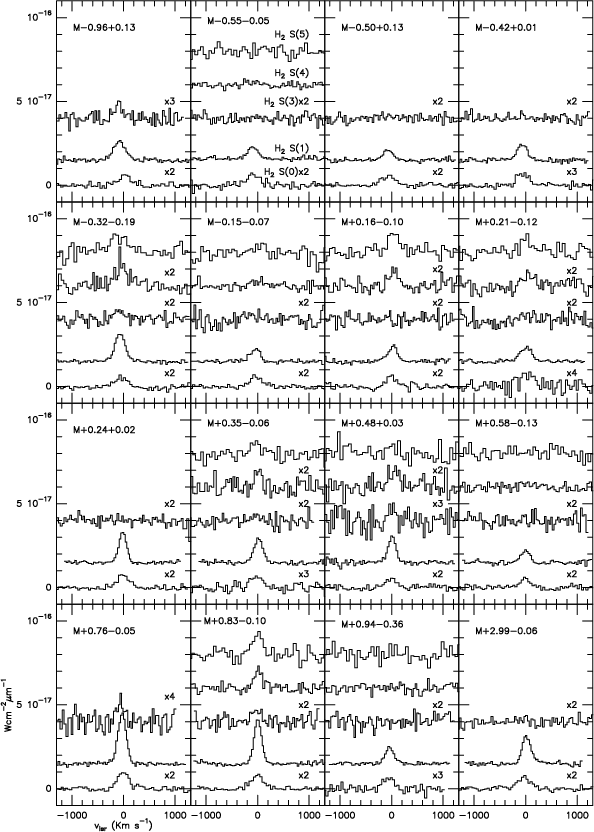Figure 3: H2 spectra. They have been rebinned to one fifth of the instrumental resolution for point sources

The absolute flux calibration errors are less than 30, 20, 25, 25, and 15% for the S(0), S(1), S(3), S(4), and S(5) lines, respectively (Salama et al. 1997). Because of the medium spectral resolution of the SWS02 mode ( $\lambda/ \Delta\lambda \sim1000$-2000) and the wavelength calibration uncertainties ($\sim \,$15-50 kms^-1 depending on the wavelength, see Valentijn et al. 1996), it is difficult to undertake a detailed comparison between the kinematics of the lines and those of the and lines. Table 3 lists the radial velocities of the S(1) lines, which have the higher signal-to-noise ratio. Within the calibration uncertainties, the radial velocity of the lines agrees with at least one of the components listed in Table 2.

Unfortunately, the lack of resolution does not allow us to establish if the emission is indeed arising from just one or several of the CO velocity components since, in general, all of them are within the velocity range of the unresolved emission. M -0.96+0.13 is the only cloud for which we can say that the warm is not likely to arise in all the velocity components seen in CO. The CO components are centered at -110, 11, and 133 kms^-1, while the S(1) line is centered at -70 kms^-1. Even with the spectral resolution of the SWS02 mode, one can see that the CO component with forbidden velocities (133 kms^-1) is not likely to contribute to the emission.

Table 3 also lists the widths of the  S(1) lines. The   line widths of the GC clouds tend to be larger than the instrumental resolution for extended sources ($\sim \,$170 kms^-1 for the S(1) line, see Lutz et al. 2000). This is due to the large intrinsic line widths typical of the GC clouds and mainly, to the presence of several velocity components along the line of sight that contribute to the emission. However, not all the sources that show CO emission in several velocity components have line widths larger than $\sim \,$170 kms^-1 (for instance M +0.83-0.10 or M +0.16-0.10). This implies that not all the CO velocity components detected in these sources are contributing to the emission, although it is difficult to discriminate which ones are emitting in .