A&A 365, 144-156 (2001)
DOI: 10.1051/0004-6361:20000174
Search for NH3
ice in cold dust envelopes around YSOs
E. Dartois1 - L. d'Hendecourt2
Send offprint request: E. Dartois,
1 - Institut de RadioAstronomie Millimétrique (UPS2074),
300 rue de la piscine, 38406 Saint Martin d'Hères, France
2 -
Institut d'Astrophysique Spatiale (MR8617), Bât. 121, Université Paris XI, 91405 Orsay Cedex, France
Received 28 July 2000 / Accepted 29 September 2000
Abstract
We present a study of the 3.1 micron absorption band, attributed to the OH stretching mode of the water molecule in the form of solid ice, observed in many protostellar lines of sight by the SWS instrument on board ISO. Using ice optical constants and Mie theory, we obtain reasonable fits
to the peculiar band shapes observed in twelve sources. The fits clearly show that some scattering effects arise in this absorption band, as the grain sizes used in the calculations are of the order of a few tenths of a micron. In the fit residuals, we search for the  1 and 3 vibrations of
the ammonia molecule which fall in the same spectral region, leading only to upper limits for the NH3 content of a few percents of the total water ice content in these different lines of sight. We also discuss the occurrence of a 3.47
1 and 3 vibrations of
the ammonia molecule which fall in the same spectral region, leading only to upper limits for the NH3 content of a few percents of the total water ice content in these different lines of sight. We also discuss the occurrence of a 3.47  m absorption band which could be related to the formation of an ammonia hydrate in the ice mantles. On the assumption that this band is due merely to this hydrate and with the help of relevant laboratory experiments, we show that
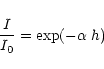
ammonia represents therefore at most 5% in abundance relative to water ice in these interstellar grain mantles. Finally, this study sheds light on the "3.1 m/6 m column density paradox" obtained when comparing the water ice absorption band at 3.1 (stretching mode) and 6 m (bending mode). We show that this paradox is resolved by considering different extinction regimes, in which scattering affects only the 3.1 m band whereas pure absorption dominates at 6 m.
m absorption band which could be related to the formation of an ammonia hydrate in the ice mantles. On the assumption that this band is due merely to this hydrate and with the help of relevant laboratory experiments, we show that
ammonia represents therefore at most 5% in abundance relative to water ice in these interstellar grain mantles. Finally, this study sheds light on the "3.1 m/6 m column density paradox" obtained when comparing the water ice absorption band at 3.1 (stretching mode) and 6 m (bending mode). We show that this paradox is resolved by considering different extinction regimes, in which scattering affects only the 3.1 m band whereas pure absorption dominates at 6 m.
Key words: ISM: clouds - dust, extinction - ISM: lines and bands - ISM: magnetic fields
Author for correspondance: dartois@iram.fr
1 Introduction
Nitrogen cosmic abundance is high (
 N
N ,
Snow & Witt 1996), and the presence of solid state molecules
containing this atom appears therefore logical.
Hydrides of the most abundant elements O, C and N, in the form of H2O,
CH4 and NH3 were proposed as early as
1949 by van de Hulst and models of molecular cloud chemistry involving gas and grains interactions clearly showed that these species should be made and stored, at least partially, on interstellar grain mantles (Tielens 1982; d'Hendecourt et al. 1985). The detection of a strong absorption band at 3.1 micron in the mid 70's was firmly attributed to water ice, on the basis of laboratory experiments (Léger et al. 1979) followed by many others (Hagen et al. 1983; Smith et al. 1989) as well as further observations (Willner et al. 1982; Whittet 1983).
,
Snow & Witt 1996), and the presence of solid state molecules
containing this atom appears therefore logical.
Hydrides of the most abundant elements O, C and N, in the form of H2O,
CH4 and NH3 were proposed as early as
1949 by van de Hulst and models of molecular cloud chemistry involving gas and grains interactions clearly showed that these species should be made and stored, at least partially, on interstellar grain mantles (Tielens 1982; d'Hendecourt et al. 1985). The detection of a strong absorption band at 3.1 micron in the mid 70's was firmly attributed to water ice, on the basis of laboratory experiments (Léger et al. 1979) followed by many others (Hagen et al. 1983; Smith et al. 1989) as well as further observations (Willner et al. 1982; Whittet 1983).
The ISO satellite, observing above the atmosphere has fully confirmed the presence of massive amounts of H2O ice in the spectra of many protostars as well as of other solid state species such as CO, CO2, CH4
(d'Hendecourt et al. 1996; Schutte et al. 1996; Gerakines et al. 1999; Boogert et al. 2000). Yet, solid-state nitrogen containing species remain quite elusive and the detection of ammonia ice remains controversial. However, the ammonia molecule is detected since a long time in the gas phase in molecular clouds (e.g. Cheung et al. 1969), with relatively high abundances respective to H2 (10
-7-10-8, Ho & Townes 1983; Turner 1995).
Before ISO, laboratory studies using astrophysical ice mixtures (Hagen
et al. 1983) have provided constraints on the shape of the 3.1 micron absorption
band by using mixtures of water and ammonia. Van de Bult et al. (1985) confirmed this constraint using Mie calculations on H
 mixtures. However, it should be noted that ground based observations (Smith
et al. 1989) obtained a low upper limit of only 2% of ammonia in two
sources (BN and GL989). The upper limit placed by Whittet et al. (1996) in HH100-IR
is only 8%, and the discussion on the detectability of this band under low mixing ratios with water ice questioned.
mixtures. However, it should be noted that ground based observations (Smith
et al. 1989) obtained a low upper limit of only 2% of ammonia in two
sources (BN and GL989). The upper limit placed by Whittet et al. (1996) in HH100-IR
is only 8%, and the discussion on the detectability of this band under low mixing ratios with water ice questioned.
Detection of ammonia ice has been claimed by Lacy et al. (1998) through the observation of its umbrella mode located in the wing of the strong silicate feature observed in the NGC 7538 IRS9 young stellar source. In the same paper however, no detection is reported for the other objects studied. ISO SWS data of the same source does not show the same optical depth in
this peculiar feature. One of the difficulties in the interpretation of this band lies in the high abundance of methanol in NGC 7538 IRS9, at a level of 10% of water ice, which contributes significantly to the optical depth in this spectral region. The derived abundance of ammonia in this source (10%) must be confirmed by the observation of other bands. Indeed, when the silicate band is extracted, there still exist two additional adjacent lines of methanol (located at 8.85 and 9.75 m) to extract. Therefore, the exact percentage of NH3 has to be taken with care as an uncertainty of 100% would be easily hidden in the saturation effects. Recently, Chiar et al. (2000) claimed the detection of very large amounts of ammonia (20-30%) in ice mantles toward Galactic Centre sources. We show, in the remaining of this paper that this detection is indeed questionable.
A low abundance of ammonia may result from locking of nitrogen in the form of N2, as suggested by the model calculations of d'Hendecourt et al. (1985), where, after the complete transformation of atomic hydrogen in H2, hydrides are not formed so efficiently and species such as O2 and N2 start to dominate the overall ice mantle composition. N2 being almost totally unobservable in the IR, its vibration band (weakly activated by interactions in an ice mixture, like O2, Ehrenfreund et al. 1992) falls right on the deep absorption of CO2, a solid state feature ubiquitous in the ISM (de Graauw et al. 1996).
Finally, the last and rather important aspect of the search for solid state ammonia is linked to the presence of a strong absorption band located at 4.62 m in many protostellar sources. This band was easily reproduced in laboratory experiments involving photochemical evolution of ice mixtures, as early as its discovery (Lacy et al. 1984). Tentatively attributed to a CN stretching mode by d'Hendecourt et al. (1986) in a unspecified species, its identification to the OCN-ion was convincingly made in subsequent laboratory experiments (Grim & Greenberg 1987; Schutte & Greenberg 1997;
Demyk et al. 1998;
Pendleton et al. 1999;
Palumbo et al. 2000 and references therein).
It is, until now, the best hint for the presence of nitrogen containing species in grain mantles. Laboratory mixtures used to photochemically produce the species at the origin of this band make a large use of ammonia and CO. Thus, constraints on the abundance of ammonia in interstellar ices appear a powerful tool to understand the overall chemistry (e.g. photochemistry, ion bombardments or surface chemistry) of molecular mantles in the ISM.
In this paper, we first present the ISO-SWS data set of young stellar
objects observations. We then focus on the reduction procedure used to
obtain an homogeneous sample of objects. The observations are then fitted
using Mie theory and we search for NH3 absorptions in the fit residuals.
Negative results of this search are discussed. We show that if ammonia is
present, the formation of an hydrate of ammonium takes place that is
responsible for the formation of a weak band at 3.47 m, a band that is
observed in many objects (Allamandola et al. 1992; Brooke et al. 1996) as well as in some of the objects in our sample. If our interpretation is
correct, then an amount of about 5% of ammonia at most can be deduced from
our spectral analysis.
A byproduct of this study is to propose a
simple explanation to the problem of the discrepancy obtained in water
ice column densities derived when interpreting two different modes at 3.1
and 6 m.
2 Observations and data reduction
The spectra presented here come from the ISO data archive (http://www.iso.vilspa.esa.es/). We have reduced moderate resolution (SWS01) and high resolution (SWS06) spectra in the following manner. The simple method discussed here makes sure that any feature discussed is not contaminated by a bad detector response or a misalignment between sub-bands that cover the observed very broad band, which must be taken into account when broad solid state features are
considered.
The ISO observing mode recorded the spectra with a grating, scanning wavelengths alternatively in the increasing and decreasing wavelength directions, the resultant spectrum being the sum of at least one "upward'' and one "downward'' scan. When a strong flux gradient in the observed band, or a strong narrow line (such as an H2 or HI line) is present, some memory effects can affect the final spectrum and upward and downward scans are not superimposable. Moreover, when looking at broad
bands, such as the water ice modes, the spectrum is constructed with sub-bands from different detectors that overlap and whose aperture in the sky can change, depending on the sub-band considered. Consequently, the sum of the two scans may not be representative of the true flux.
To disentangle these effects, during the reduction we separate the downward scans from the upward ones. In doing so, we lose a factor
 in the signal-to-noise ratio, but we get in return two individual scans that must be identical (above the signal-to-noise ratio), any deviation in one scan being considered as a bad behaviour. The limits we will derive hereafter are therefore conservative. To be sure that no problem arises in the overlapping of two sub-bands, we decide to use a gain correction in a small overlapping region between bands (a few percent of the total bandwidth). If two scans overlap in a small spectral region, we calculate the average of the flux in the wavelength region they have in common and apply a multiplying factor to the second scan so that the overlapping regions match in flux. This correction is especially needed in the case of the NH3 stretching modes which are located near the overlapping of the ISO-SWS 1b and 1d band. All these corrections, as well as the resulting spectra in
upward and downward scans are presented in Fig. 1.
in the signal-to-noise ratio, but we get in return two individual scans that must be identical (above the signal-to-noise ratio), any deviation in one scan being considered as a bad behaviour. The limits we will derive hereafter are therefore conservative. To be sure that no problem arises in the overlapping of two sub-bands, we decide to use a gain correction in a small overlapping region between bands (a few percent of the total bandwidth). If two scans overlap in a small spectral region, we calculate the average of the flux in the wavelength region they have in common and apply a multiplying factor to the second scan so that the overlapping regions match in flux. This correction is especially needed in the case of the NH3 stretching modes which are located near the overlapping of the ISO-SWS 1b and 1d band. All these corrections, as well as the resulting spectra in
upward and downward scans are presented in Fig. 1.
![\begin{figure}
\par\includegraphics[bb=7 207 593 540,width=8.1cm,clip]{ds10157f1...
...m}
\includegraphics[bb=7 207 593 540,width=8.1cm,clip]{ds10157f8.ps}\end{figure}](/articles/aa/full/2001/02/aa10157/Timg12.gif) |
Figure 1:
a)
ISO SWS spectra of the young stellar objects studied, after data reduction.
The upward and downward scan are shown side by side. The lower curve in each panel
is the spectrum without applying any stitching factor in the overlapping region of
each sub-band of the spectrum, reduced individually. It can cause a shift such as the
one observed in the Orion spectrum at 3.5 m. The upper spectrum is the same when
an overlapping gain correction has been applied, and the fitted curve is the best
estimate for the continuum of the source |
| Open with DEXTER |
![\begin{figure}
\par\includegraphics[bb=7 207 583 540,width=8cm,clip]{ds10157f9.p...
...m}
\includegraphics[bb=7 207 593 540,width=8cm,clip]{ds10157f12.ps}
\end{figure}](/articles/aa/full/2001/02/aa10157/Timg13.gif) |
Figure 1:
b) Same as in a)
the sources with no data in between
3.5 and 3.98 m are high resolution ISO data (SWS06) |
| Open with DEXTER |
![\begin{figure}
\par\includegraphics[bb=96 373 542 692,width=8.8cm,clip]{ds10157f...
...r\includegraphics[bb=93 372 542 692,width=8.8cm,clip]{ds10157f14.ps}\end{figure}](/articles/aa/full/2001/02/aa10157/Timg14.gif) |
Figure 2:
Real and imaginary part of the complex refractive index of water ice in the 3 m OH stretching mode region for various sample degree of crystallisation. From top to bottom the spectra are recorded at 10, 15, 30, 50, 80, 120 and 160 K. The last one is at 60 K (see text for explanation). For clarity the spectra have been shifted. The reference in the upper panel is the upper curve and in the lower panel  at 4 m for each curve
 |
| Open with DEXTER |
3 Spectra modelling
The 3 micron astronomical water ice band appears to be relatively broader in the observed
sources than the one measured in laboratory transmittance spectra. Furthermore,
the observed asymmetry (Fig. 1) giving a more extended red wing is typical
of what is expected from scattering of light by particles that approach a size
comparable to the wavelength (see Bohren & Hoffman 1983 for a comprehensive
description).
We know from the rest of the infrared
protostellar spectra that good fits to the data can be obtained
using thin film spectra measured directly in the laboratory,
without taking care of scattering effects, in the bands observed at
wavelengths above  5 microns (d'Hendecourt et al. 1998).
The important parameter when discussing the possible scattering effects is
 which must remain
  ,
m being the complex refractive index of the material considered, in order to neglect scattering and consider only pure absorption.
,
m being the complex refractive index of the material considered, in order to neglect scattering and consider only pure absorption.
These considerations tend to point out that the grain size distribution must contain grains of the order of
 to 0.5 m for scattering to affect the shape of the 3 m band (typical index of refraction of ices in this wavelength region lies between 1. and 1.5).
To investigate the effects of scattering of such
grains on the spectra we use a Mie scattering code,
developed by Bohren & Huffman (1983). This
code allows us to derive the extinction coefficients
(
 )
in the case of a coated spherical particle. To run this program we need to specify the complex index of refraction of the
material in the core and in the mantle of the grain, as well as the respective grain radius for each component. We use here the classical Draine and Lee optical constants (1984) for the silicate core of the grain. As there is no strong transition from silicates falling in this spectral region, modifying the kind of silicates used for the core will not strongly affect the results presented here. For the ice mantle we need more refinements to explain the various line shapes observed. In particular we need to specify precisely its degree of crystallisation (associated with the temperature of the grains). For this, we use the constants carefully derived by Schmitt et al. (1998) for the extreme ice temperature components. For intermediate temperatures we calculate the optical constants from pure transmittance spectra recorded in the laboratory (from Institut d'Astrophysique Spatiale, Orsay, France and University of Leiden, The Netherlands).
)
in the case of a coated spherical particle. To run this program we need to specify the complex index of refraction of the
material in the core and in the mantle of the grain, as well as the respective grain radius for each component. We use here the classical Draine and Lee optical constants (1984) for the silicate core of the grain. As there is no strong transition from silicates falling in this spectral region, modifying the kind of silicates used for the core will not strongly affect the results presented here. For the ice mantle we need more refinements to explain the various line shapes observed. In particular we need to specify precisely its degree of crystallisation (associated with the temperature of the grains). For this, we use the constants carefully derived by Schmitt et al. (1998) for the extreme ice temperature components. For intermediate temperatures we calculate the optical constants from pure transmittance spectra recorded in the laboratory (from Institut d'Astrophysique Spatiale, Orsay, France and University of Leiden, The Netherlands).
To calculate the constants, we assume that the transmittance is given by the classical equation:
where
 is the imaginary part of the complex index of refraction and
  is the wavelength.
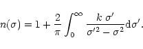
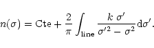
We calculate the refractive index n using the Kramers-Kronig (Bohren & Huffman) relation:
This equation must be integrated over the entire electro-magnetic range. In practice,
if the modes are well separated in energy, only the adjacent frequencies in the
absorption considered are, to first order, important to determine the integral,
the other modes being considered as providing a constant contribution. Therefore
we can decompose the integral in two parts and consider that:
For the constant we adopt a mean value of 1.28 (From Trotta and Schmitt's data).
The resultant optical constants used for the Mie calculations are presented in Fig. 2 for water ice. They are presented in increasing temperature order (from 10 K to 160 K from top to bottom), except for the last one which is entirely crystalline, but have been annealed and measured at 60 K. This last spectrum is however representative of the totally crystalline ice band. Note that the main effect in changing the constant is the crystallinity. The constants we calculate are not determined with the same accuracy as the ones of Trotta and Schmitt, but are sufficient for the study we present hereafter.
To represent the variation in temperature of the ice mantle we do not use the constants as they are, but rather use the Maxwell-Garnett theory to produce mean optical constants for an ice mantle including several ice phases. This theory allows us to calculate the average dielectric function of mixed materials embbeded in a matrix, the other constituents being inclusions. The Maxwell Garnett average dielectric function is given by:
where f is the total fraction of constituent by volume,
 the matrix dielectric function,
 the dielectric function of the jth inclusion and
  is a function related to the shape probability function of the inclusions. When the inclusions are
spherical (which we adopt here) this function is simply given by
is a function related to the shape probability function of the inclusions. When the inclusions are
spherical (which we adopt here) this function is simply given by
 .
.
This dielectric function
 is easily related to n+ik through the constitutive relations:
Once we have calculated the mean complex index of refraction of the
ice mantle, using the Mie program "bhcoat''
(Bohren & Huffman 1983), we then produce
 .
It is related to the optical depth by:
.
It is related to the optical depth by:
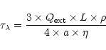
where L is the length of the line of sight,
the extinction coefficient,  the density of grains in space, a the radius of the grain and
  the specific density of the grain (Whittet 1992). The silicate absorption rises rapidly in this wavelength range. To
compare the observation to the model we therefore
extract the ice band exactly in the same way
as in the observation. We therefore take
the specific density of the grain (Whittet 1992). The silicate absorption rises rapidly in this wavelength range. To
compare the observation to the model we therefore
extract the ice band exactly in the same way
as in the observation. We therefore take
 ,
where
,
where  is the
conversion factor between the visual extinction AV
and extinction at 2.5 m. We assume
to be
of the order of
is the
conversion factor between the visual extinction AV
and extinction at 2.5 m. We assume
to be
of the order of  ,
following the extinction
curve for the MRN mixture in Fig. 8 of the Draine & Lee paper (1984).
,
following the extinction
curve for the MRN mixture in Fig. 8 of the Draine & Lee paper (1984).
To extract the transmittance spectrum, we fit the same order polynomial as the one
we used to extract the water ice band in the ISO observations. An example of the
procedure is shown for the Orion BN case in Fig. 3, assuming AV for this
object is 17 (Gezari et al. 1998).
![\begin{figure}
\par\includegraphics[bb=92 125 594 651,width=6.6cm,clip]{ds10157f...
...r\includegraphics[bb=79 125 594 651,width=6.6cm,clip]{ds10157f17.ps}\end{figure}](/articles/aa/full/2001/02/aa10157/Timg40.gif) |
Figure 3:
Processus of extraction of the transmittance spectra after Mie
calculation with an extinction corresponding to the Orion case. Dashed lines
represent the pure absorption case and full line the total extinction case
(absorption + scattering). Upper left panel: transmittance spectra.
Upper right panel:
transmittance spectra multiplied by a blackbody (500 K) corresponding to the
source continuum, as is observed in the interstellar case. Note that absolute
scales are represented (no shifts are applied). Lower panel: resultant optical
depths derived in the case of pure absorption and extinction as well as the
corresponding differential extinction (dotted line) |
| Open with DEXTER |
To illustrate the effect of the continuum extraction as well as scattering,
we show this extraction in the case we take into account only the absorption
coefficient
 and the case of the full extinction
.
We first present the fit obtained extracting directly the optical depth from
and the case of the full extinction
.
We first present the fit obtained extracting directly the optical depth from
 .
However in the observations we measure a flux corresponding to
.
However in the observations we measure a flux corresponding to
 ), where
 )
is the Planck function at temperature T. That is why the spectra present
a steep rise with wavelength. Therefore to show that our
fit in the upper panel is correct, we present just below the same curves (fit and transmittance) multiplied by a blackbody of 500 K, typical of the apparent temperature of the underlying continuum source. The final optical depths derived in both cases (with total extinction or just absorption) as well as the corresponding optical depths differences are presented below to clearly denote the effects of scattering. Of course all of this approach is not what would require the full radiative transfer treatment of the problem. However, it allows us to show we can explain to first order the entire water ice mode with the combination of different temperatures and simple scattering effects, without adding any other compound opacity.
)
is the Planck function at temperature T. That is why the spectra present
a steep rise with wavelength. Therefore to show that our
fit in the upper panel is correct, we present just below the same curves (fit and transmittance) multiplied by a blackbody of 500 K, typical of the apparent temperature of the underlying continuum source. The final optical depths derived in both cases (with total extinction or just absorption) as well as the corresponding optical depths differences are presented below to clearly denote the effects of scattering. Of course all of this approach is not what would require the full radiative transfer treatment of the problem. However, it allows us to show we can explain to first order the entire water ice mode with the combination of different temperatures and simple scattering effects, without adding any other compound opacity.
4 Results
The resultant extracted best spectra, comparing the results of the model to the observations, are presented in Fig. 4. To produce the model spectra, we used grains whose total size is of the order of 0.1 to 0.5 micron and whose core radius is of the order of 0.05 to 0.4 micron. We used single sized grains, without taking into account any size distribution.
This probably explains why there still exists some lack of extinction in part of
the red wing of the band. However, in some cases (e.g. SGRA*, IRAS 17424),
the 3.4 m absorption band is clearly due to the presence of an aliphatic organic component.
In almost all other sources a right wing as well as a
band at 3.47 m remains, the later one thoroughly studied by Brooke &
Sellgren (1999) in numerous objects. As emphasised by
the authors, this band appears to be correlated with the water ice band.
We do not claim our fits to be unique. They are intended to demonstrate
that the whole band can be adjusted by water ice at various states of
crystallinity. Because of the interplay between too many physical parameters,
we believe that the problem cannot be simply inverted and the exact parameters
of the band (size distribution, exact ice temperature, ...)
extracted. However, these fits allow us to search for the NH3
stretching mode absorption bands in the residuals between the fit and
the observation, as shown in the upper part of each panel of Fig. 4.
We do not detect any convincing band which could be attributed to
NH3 in any source, and estimate an upper limit on its abundance in
the following manner. We calculate the
2 level of the residual of
the fit in the interval of the band for the upward and downward scans separately.
We multiply this by the expected width of the feature (40 cm-1). We obtain in
this way an integrated absorbance. The ammonia spectra corresponding to the
maximum contribution to the residual are presented for each source in
Figs. 4a and 4b (upper traces, one for each wavelength scanning directions).
level of the residual of
the fit in the interval of the band for the upward and downward scans separately.
We multiply this by the expected width of the feature (40 cm-1). We obtain in
this way an integrated absorbance. The ammonia spectra corresponding to the
maximum contribution to the residual are presented for each source in
Figs. 4a and 4b (upper traces, one for each wavelength scanning directions).
![\begin{figure}
\par\includegraphics[bb=57 207 548 540,width=8cm,clip]{ds10157f18...
...ps}\includegraphics[bb=42 207 548 540,width=8cm,clip]{ds10157f25.ps}\end{figure}](/articles/aa/full/2001/02/aa10157/Timg46.gif) |
Figure 4:
a) 3 micron optical depth spectra of the young stellar objects used in this study. The ISO-SWS upward and downward scans are separated and fitted with the same spectra (see text). The residual of the fit is presented in the upper part of each panel. For comparison, the spectrum of pure NH3 ice is presented in the top of the residuals, with a depth corresponding to its maximum allowed contribution |
| Open with DEXTER |
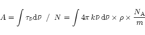
In parallel we integrate the fit performed on the water ice band and derive the ratio of the resulting two integrated absorbances. This is done for each scan direction. We did not only fit the region where the 2.97 m feature occurs, but the whole water ice stretching mode, i.e. including the red part of the absorption for example that is not reproduced e.g. in the Chiar et al. (2000) analysis. To derive a more stringent upper limit on NH3 we would have to ask what
H2O ice parameters allow the largest amount of NH3, and not what parameters allow the best fits of the spectra without
NH3. However, we believe that the global fit performed gives a good representation of the real state of water ice in all the wavelength range of the spectrum in the region free of NH3 lines, and that it is therefore very close to the actual water ice absorption.
If we multiply the integrated absorbances ratios derived by the ratio of the
measured integrated absorption coefficient of the H2O and NH3 stretching modes,
we are then able to derive the maximum percentage of ammonia undetected
in the water ice. Note that this ratio can vary upon the mixture involved. We have
searched for values in the literature for the NH3 stretching mode absorption
coefficient. The one determined by d'Hendecourt et al. (1986)
is
 cmmol-1. We also
determine this absorption
coefficient using the relation:
cmmol-1. We also
determine this absorption
coefficient using the relation:
where N is the column density of absorbers, k the imaginary part of the complex index of refraction,  the wavenumber,
the density of the material,
the wavenumber,
the density of the material,  the Avogadro's number and m the molecular weight of the constituent considered. Using the constants by Mukai & Krätschmer (1986) and
  gcm-3, we obtain
 cmmol-1.
Table 1:
Integrated absorbance ratios and NH3/H2O upper limit. Note that the highest upper limits are only governed by the signal-to-noise
| Source name |
up |
down |
upper limit |
| |
ratio (%) |
ratio (%) |
NH3/H2O |
| SGRA* |
0.71 |
0.71 |
<11-17% |
| S140 |
0.23 |
0.22 |
<3.4-5.3% |
| Orion |
0.31 |
0.27 |
<4.4-6.9% |
| NGC 7538 IRS1 |
0.93 |
1.20 |
<16-25% |
| IRAS 17424 |
0.82 |
0.75 |
<12-19% |
| GL989 |
0.31 |
0.29 |
<4.5-7.1% |
| GL490 |
0.83 |
0.74 |
<12-19% |
| GL2591 |
0.42 |
0.57 |
<7.4-12% |
| GL2136 |
1.19 |
0.94 |
<16-25% |
| NGC 2024 IRS2 |
0.40 |
0.47 |
<6.5-10% |
| RCRA |
1.25 |
1.07 |
<17-27% |
| ELIAS 16 |
0.70 |
0.63 |
<9.9-15% |
For water ice, d'Hendecourt et al. (1986) and
Gerakines et al. (1995)
determined
 10-16 cmmol-1
whereas Hudgins et al. (1993) gives (
10-16 cmmol-1
whereas Hudgins et al. (1993) gives (
 cmmol-1), depending on the two interstellar ice mixtures they studied.
We adopt the extreme values for the ratio of integrated absorbance of H2O/NH3, leading to a multiplicative factor of 15-24. This number must be multiplied by the integrated ratio measured on the spectra to derive the NH3 to H2O percentage upper limit. The results of the analysis are summarised in Table 1.
We emphasise here that the overall quality of ISO-SWS spectra on
these faint objects does not allow a very constraining upper
limit on the quantity of ammonia as the derived upper
limits are mostly due to the ultimate signal-to-noise
of the spectra. Ground based spectra in the 3
micron window, such as the ones discussed by Brooke et al.
(1999), provides a better S/N data in this range.
Yet no detection of any ammonia features at
 m is reported in this set of data, and none of the spectra seem to present any feature in this wavelength range.
5 Indirect observation of ammonia?
Among the infrared absorptions detected toward young stellar objects, resides a well known 3.47 m feature. This absorption can be studied from the ground as it falls in a spectral region almost free of H2O vapour. It was first observed and discussed by Allamandola et al. (1992), which attributed it to a CH stretch on a diamond surface. Since then, it has been systematically studied in many molecular clouds by Sellgren et al. (1994), Brooke et al. (1996), Brooke et al. (1999). It was also reported in two Taurus sources by Chiar et al. (1996). In 1996, Brooke et al. showed that the optical depth of this feature is correlated with H2O ice, a trend that is confirmed in their recent study (Brooke et al. 1999).
In parallel, in the laboratory, when ice mixtures containing H2O and NH3 are deposited at low temperature, an additional absorption arises on the red wing of the water ice stretching mode feature. This new mode is in fact the consequence of the formation of an ammonia monohydrate in the matrix. We present here a laboratory study that shows that this band should participate to the unidentified 3.47 m band. It would fulfill all the requirements as compared to observations, that is to say:
- It correlates with water ice and not with silicates, which means it is formed altogether with the water ice in proportions that do not vary by huge factors from source to source, as is the case for CO2 (de Graauw et al. 1996);
- No other new band has been claimed to be correlated with this one in the full infrared spectra of young stellar objects (YSOs) recorded by ISO spectrometers;
- It presents no substructures, which seems to reject a possible identification with aliphatic C-H bonds.
NH3 is actually known to form hydrates with H2O (Sill et al. 1980; Bertie & Morrison 1980; Mukai & Kratschmer 1985). As ice mantles on top of interstellar grains are dominated by water ice, we therefore expect such hydrates to be present if ammonia is indeed present in the ice. One of the main bands that is apparent when the formation of H2O.NH3 hydrate occurs in the ice is the
(O-H ... N) mode around
2900 cm-1 (3.45 m). This new mode is due to
the perturbation by ammonia molecules of the water
ice stretching frequency, following the length of the
(O-H ... N) hydrogen bond formed. To first order, it should not influence the 2.97 m feature's integrated absorption cross section.
![\begin{figure}
\par\includegraphics[angle=90,bb=64 21 536 753,width=12cm,clip]{ds10157f30.ps}\end{figure}](/articles/aa/full/2001/02/aa10157/Timg60.gif) |
Figure 5:
Temperature evolution of the water-ammonia ice mixture. The spectra are shown
in two individual wavelength windows to allow the best dynamic range to clearly see
the overall spectrum (note the different vertical scales). The vertical dashed lines
indicate the ammonia and hydrate stretching modes, respectively at 2.97 and 3.47 m.
Other ammonia modes lies at
 m on top of the water ice bending mode
and at m on top of the water ice bending mode
and at
 m (umbrella mode) m (umbrella mode) |
| Open with DEXTER |
![\begin{figure}
\par\includegraphics[angle=90,bb=46 70 530 747,width=8.6cm,clip]{...
...egraphics[angle=90,bb=46 70 530 747,width=8.6cm,clip]{ds10157f33.ps}\end{figure}](/articles/aa/full/2001/02/aa10157/Timg61.gif) |
Figure 6:
Laboratory spectra of H2O:NH3 mixtures where the abundance of NH3 represent from 0 to 7% of the water ice content. The spectra are recorded at various temperatures (10 K, 80 K and 160 K from top panel to bottom panel) to show the effects of crystallisation. The lower spectrum of each panel is the superposition of a pure H2O spectrum and the H2O:NH3-100:7 one. The grey region put the emphasis on the difference of the spectra, showing the presence of the 3.47 m hydrate mode indicated by a vertical arrow. In the highest temperature spectrum, the band is weaker due to the partial evaporation of some of the NH3 ice. The dashed line indicate the position of the NH3 stretching mode which is only fully discernible from the water ice band in the 7% mixture at 10 K. It also demonstrate the difficulty in its detection due to the water ice crystallisation |
| Open with DEXTER |
Under very low mixing ratios, the ammonia modes will be very difficult to
detect in astronomical spectra. The strongest one around 9 m (2,
umbrella mode) will form part of the silicate absorption band. To retrieve it,
we then need to obtain high signal to noise spectra in this region
and to be able to precisely evaluate the underlying silicate and other ices
absorptions. Given the width of this feature (see Fig. 5), it is a very difficult task.
Let us now focus on the deformation modes (6.2 m).
They fall in the water ice bending mode and their spectral
signature vanish in the ice band,
if ammonia is not present at least at the 5-10% abundance level relative to water ice.
Similar processes affect the N-H stretching modes (2.97 m) which will suffer
from both effects (contrast and optical depth), due to its presence in the water ice
stretching mode wing.
m) which will suffer
from both effects (contrast and optical depth), due to its presence in the water ice
stretching mode wing.
To illustrate the points discussed above, we present in Fig. 5
the spectra of H2O:NH3 mixtures at a dilution level of 7%.
The intended dilution is monitored afterward by measuring the integrated
absorbances of the NH3 umbrella mode at 9 m and comparing it to the 6 m bending mode of water ice. The respective integrated cross sections are of
 cmmol-1 and
 cmmol-1 (d'Hendecourt et al. 1986). We therefore deduce the dilution to be 7%. The spectra are presented at three temperatures to show the temperature evolution of the features. At 10 K, in the left panel, the small bump at 2.96 m in the water ice stretching mode is due to the NH3 stretching mode. When the temperature of the sample is raised, the observed band is dominated by the water ice crystallisation
shoulder.
cmmol-1 (d'Hendecourt et al. 1986). We therefore deduce the dilution to be 7%. The spectra are presented at three temperatures to show the temperature evolution of the features. At 10 K, in the left panel, the small bump at 2.96 m in the water ice stretching mode is due to the NH3 stretching mode. When the temperature of the sample is raised, the observed band is dominated by the water ice crystallisation
shoulder.
In Fig. 5, a new (large) absorption appears in the spectrum around 3.5 m,
indicated by a vertical dashed line. This band is due to the ammonia hydrate.
In Fig. 6 we present a close-up on the
 m spectral region of
water ice spectra containing from zero to seven percent of ammonia. The lowest
spectrum of each panel is the superposition of the water ice mode and the 7%
spectrum. The difference is shaded to evidence the hydrate band. From this
difference we can evaluate the integrated absorbance of the pure water ice
and compare it to the hydrate one. The ratio of the two bands is almost the
same as the ratio of NH3 to H2O abundance in the mixture, indicating
that the hydrate integrated cross section is of
m spectral region of
water ice spectra containing from zero to seven percent of ammonia. The lowest
spectrum of each panel is the superposition of the water ice mode and the 7%
spectrum. The difference is shaded to evidence the hydrate band. From this
difference we can evaluate the integrated absorbance of the pure water ice
and compare it to the hydrate one. The ratio of the two bands is almost the
same as the ratio of NH3 to H2O abundance in the mixture, indicating
that the hydrate integrated cross section is of
 cmmol-1.
6 The 6
 m to 3
m ice band ratio paradox
m to 3
m ice band ratio paradox
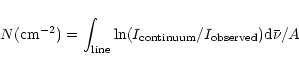
We address in this section an interesting byproduct of our study. To derive ice column densities in interstellar spectra one generally draws a local continuum on both sides of the band to integrate, taking ln(
 )
and use the fact that:
)
and use the fact that:
where A is the integrated absorption coefficient measured in the laboratory on a thin film. However, the occurrence of scattering, due to the low end of the dust size distribution (large sizes), in the 3 m absorption band of water ice breaks this direct correspondance. This calculation remains valid only if the size of the grains is small compared to the wavelength. To illustrate this effect, we calculate the transmittance spectra of two core-mantle grains whose size is 
 2
2 /10 (0.05 m) and for the other, comparable to the wavelength
2
(0.5 m). We extract the optical depth for the stretching and bending modes. For comparison, we have used the same normalised extinction at 2.5 m.
/10 (0.05 m) and for the other, comparable to the wavelength
2
(0.5 m). We extract the optical depth for the stretching and bending modes. For comparison, we have used the same normalised extinction at 2.5 m.
![\begin{figure}
\par\includegraphics[bb=79 368 542 702,width=12cm,clip]{ds10157f34.ps}
\end{figure}](/articles/aa/full/2001/02/aa10157/Timg74.gif) |
Figure 7:
Mie calculation of the resultant transmittance spectra of two coated grains. Upper panels: transmittance spectra obtained with two ice-silicates core-mantle grains extinction coefficients, normalised to the same total extinction for comparison. The first grain has a total radius (core + mantle) of 0.05 m (i), the second 0.5 m (ii). The respective optical depths, derived assuming the local continuum, are represented by the dotted-dashed lines are presented in the lower panels, normalised to the integrated absorbance of the 3 m stretching mode. See text for explanation |
| Open with DEXTER |
Once the spectra have been obtained, we normalise the integrated absorbance to the
3 m ice band, and apply this normalisation factor to the 6 m bending mode
extracted in both cases. We observe that the resultant spectra in the 3 m
window are not superimposed. Moreover, the 6 m bending mode spectra differ
by a multipling factor ( )
but are otherwise identical.
)
but are otherwise identical.
The direct consequence is that if one decides to use the 3 m band to evaluate the column
density of water ice, it will disagree in this case by a factor
from the estimate made at
6 m. Finally, if the 3 m band is saturated in the band center, estimating the column
density by adjusting the blue wing of the line is rather uncertain, and again a factor of two can
easily be introduced. This probably explains why, deriving the ice water column density from the
3 m band,
gives systematically a different number than the one derived from the 6 m
estimate, as noted by Allamandola et al. (1992). We emphasize here that we qualitatively demonstrate this effect by using two unique grain sizes. A full quantitative treatment of this effect must include the use of a grain size distribution as well as a proper radiative transfer model. This is beyond the scope of this paper.
7 Discussion
The absence of a clear evidence for the presence of NH3 in the ice from
the observation of the 2.97 m modes
is demonstrated for almost 20 sources
if we include both the ISO source sample presented here and the ground based
observations performed by Brooke et al. (1999). Furthermore, there
exists an intrinsic problem in the detection of this particular mode of NH3
due to the water ice mode itself. Indeed, if one looks at the H2O index of
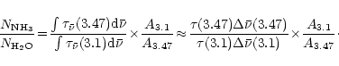
refraction imaginary part presented in Fig. 2, when ice becomes crystalline, it possesses a mode located in the very same region. The extraction task is therefore more difficult than commonly thought. Depending on the signal-to-noise ratios, the NH3/H2O abundance ratio upper limit in ice mantles ranges from 3.4 to 17%, based on the stretching modes. However, we stress that if present in ices, the ammonia molecule should interact with water to form an hydrate as shown in Sect. 5. The occurrence of the 3.47 m absorption band in many sources (Brooke et al. 1999) and in laboratory spectra is an indication that some NH3 is indeed present in the ice mantle. This band is observationally easier to detect because, although weak in interstellar spectra, it lies in a spectral region both accessible from the ground and not in the core of the water ice absorption.
We have evaluated the integrated absorption cross section of the hydrate band in the laboratory. Brooke and Sellgren have measured a correlation between the optical depths of the water ice and 3.47 m absorptions. This relation,
 ,
establishes the link in abundance between ammonia and water if the 3.47 m band is attributed to the hydrate.
,
establishes the link in abundance between ammonia and water if the 3.47 m band is attributed to the hydrate.
Working with this hypothesis, the NH3/H2O abundance ratio is therefore given by:
Using the integrated absorption cross-sections for water
ice and the one derived above for the hydrate,
the
 can been evaluated and equals
 .
Therefore the ammonia content is of 0.033 times this number, i.e.
.
Therefore the ammonia content is of 0.033 times this number, i.e.
 % in the sources used in the correlation by Brooke et al.
![\begin{figure}
\par\includegraphics[bb=42 207 548 540,width=8.8cm,clip]{ds10157f35.ps}\end{figure}](/articles/aa/full/2001/02/aa10157/Timg81.gif) |
Figure 8:
Mie calculation of the resultant transmittance spectra of a coated grain composed of a silicate core and a water:ammonia (100:4) ice mantle. The long wavelength wing is better reproduced than in Fig. 4a, which point to the possible presence of an ammonia hydrate in the mantle |
| Open with DEXTER |
Finally, Fig. 8 displays the fit obtained for GL989 with the H2O:NH3 (100:4) mixture, in the same way as done in the first sections. We are able to reproduce most of the long wavelength wing. This is not a definite detection of the hydrate as this fit relies on a single broad band, and because we neglect possible size
distribution effects. It seems however roughly in accordance with the percentage derived from the Brooke et al. correlation of this 3.47 m band with the water ice band. One must however not forget that other molecules such as H2O2 could participate to the absorption in this wavelength region (e.g. Moore & Hudson 2000).
8 Conclusions
The main conclusions of this paper are
- the absence of a clear evidence for the presence of large quantities of
ammonia in the ice mantles from the observation of the 2.97 m modes.
This result is obtained in 20 sources if we include both ISO SWS data and
the ground based observations from Brooke & Sellgren (1999).
Based on higher signal-to-noise spectra of the same source, our analysis
is in contradiction with the NH3 detection (20-30% of the water ice)
claimed by Chiar et al. (2000) toward SgrA*, whereas there could be
a few percent present in the mantle;
- A clear detection of this particular mode is hampered by confusion with a mode attributed to crystalline ice which falls precisely at the same position. It appears therefore impossible to detect with certainty low amounts of NH3 in interstellar ices through this mode;
- The presence of a broadband around 3.47 m in laboratory ice mixtures,
attributed to the formation of an ammonia hydrate allows us to propose a
tentative identification of the "3.47 m'' absorption feature detected
in previous studies. Although this identification remains tentative, we have shown that it satisfies the requirements derived from the previous observations of this band, namely that it strongly correlates with the water ice band;
- The use of this ammonium hydrate band and the laboratory measurement of its cross-section show that ammonia accounts for at most 5% of the total water ice content in most of the objects discussed in this study.
Finally, as an open question, we stress that in some lines of sight, the occurrence of an absorption band at 4.67 m is attributed to a nitrogen containing ion (OCN-). We believe that the fact we must simultaneously account for a non negligible abundance for this ion and a relatively low NH3 abundance carries an important chemical information on the evolution of ice mantles that we must further constrain.
-
Allamandola, L. J., Sandford, S. A., Tielens, A. G. G. M.,
& Herbst, T. M. 1992, ApJ, 399, 134
In the text
NASA ADS
-
Bertie, J. E., & Morrison, M. M. 1980, J. Chem. Phys., 73, 4832
In the text
NASA ADS
-
Bertie, J. E., & Morrison, M. M. 1981, J. Chem. Phys., 74, 4361
NASA ADS
-
Boogert, A. C. A., et al. 2000, A&A, 353, 349
In the text
NASA ADS
- Bohren, C. F., & Huffman,
D. R. 1983, Absorption and scattering
of light by small particles (John Wiley and Sons)
In the text
-
Brooke, T. Y., Sellgren, K., & Smith, R. G. 1996, ApJ, 459, 209
In the text
NASA ADS
-
Brooke, T. Y., Sellgren, K., & Geballe, T. R. 1999, ApJ, 517, 883
In the text
NASA ADS
-
van de Bult, C. E. P. M., Greenberg, J. M., & Whittet, D. C. B. 1985,
MNRAS, 214, 289
NASA ADS
-
Cheung, A. C., Rank, D. M., Townes, C. H., Knowles,
S. H., & Sullivan, W. T. 1969, ApJL, 157,
L13
In the text
-
Chiar, J. E., Tielens, A. G. G. M., Whittet,
D. C. B., et al. 2000, ApJ, 537, 749
In the text
NASA ADS
-
Chiar, J. E., Adamson, A. J., & Whittet, D. C. B. 1996, ApJ, 472, 665
In the text
NASA ADS
-
Draine, B. T., & Lee, H. M. 1984, ApJ, 285, 89
In the text
NASA ADS
-
Demyk, K., Dartois, E., d'Hendecourt, L., et al. 1998, A&A, 339, 553
In the text
NASA ADS
-
Ehrenfreund, P., Breukers, R., d'Hendecourt, L.,
& Greenberg, J. M. 1992, A&A, 260, 431
In the text
NASA ADS
-
Gerakines, P. A., et al. 1999, ApJ, 522, 357
In the text
NASA ADS
-
Gerakines, P. A., Schutte, W. A., Greenberg, J. M.,
& van Dishoeck, E. F. 1995, A&A, 296, 810
In the text
NASA ADS
-
Gezari, D. Y., Backman, D. E., & Werner, M. W. 1998, ApJ, 509, 283
In the text
NASA ADS
-
de Graauw, T., et al. 1996, A&A, 315, L345
NASA ADS
-
Grim, R. J. A., & Greenberg, J. M. 1987, ApJL, 321, L91
In the text
NASA ADS
-
Hagen, W., Greenberg, J. M., & Tielens, A. G. G. M. 1983, A&A, 117, 132
In the text
NASA ADS
-
d'Hendecourt, L., et al. 1996, A&A, 315, L365
NASA ADS
-
d'Hendecourt, L. B., & Allamandola, L. J. 1986, A&AS, 64, 453
NASA ADS
-
d'Hendecourt, L. B., Allamandola, L. J., & Greenberg, J. M. 1985, A&A, 152, 130
NASA ADS
-
Ho, P. T. P., & Townes, C. H. 1983, ARA&A, 21, 239
In the text
NASA ADS
-
Hudgins, D. M., Sandford, S. A., Allamandola, L. J.,
& Tielens, A. G. G. M. 1993, ApJS, 86, 713
In the text
NASA ADS
-
van de Hulst, H. C. 1949, in The solid particles in interstellar space
(Utrecht, Drukkerij Schotanus & Jens publisher), 2
-
Lacy, J. H., Faraji, H., Sandford, S. A., & Allamandola, L. J. 1998, ApJL,
501, L105
In the text
NASA ADS
-
Leger, A., Klein, J., de Cheveigne, S., et al.
1979, A&A, 79, 256
In the text
NASA ADS
-
Mukai, T., & Kraetschmer, W. 1986, Earth Moon and Planets, 36, 145
In the text
NASA ADS
-
Palumbo, M. E., Pendleton, Y. J., & Strazzulla G. 2000, AJ, 542, 890
In the text
-
Pendleton, Y. J., Tielens, A. G. G. M., Tokunaga, A.T.,
& Bernstein, M. P. 1999, AJ, 513, 294
In the text
-
Schmitt, B., Quirico, E., Trotta, F., & Grundy, W. M. 1998, Solar System Ices, 199
-
Schutte, W. A., et al. 1996, A&A, 315, L333
In the text
NASA ADS
-
Schutte, W. A., & Greenberg, J. M. 1997, A&A, 317, L43
In the text
NASA ADS
-
Sellgren, K., Smith, R. G., & Brooke, T. Y. 1994, ApJ, 433, 179
In the text
NASA ADS
-
Sill, G., Fink, U., & Ferraro, J. R. 1980, Opt. Soc. Am. J., 70, 724
In the text
NASA ADS
- Sill, G., Fink
U., & Ferraro, J. R. 1981, J. Chem. Phys., 74, 997
NASA ADS
-
Smith, R. G., Sellgren, K., & Tokunaga, A. T. 1989, ApJ, 344, 413
In the text
NASA ADS
-
Snow, T. P., & Witt, A. N. 1996, ApJL, 468, 65
In the text
-
Tielens, A. G. G. M., & Hagen, W. 1982, A&A, 114, 245
In the text
NASA ADS
-
Turner, B. E. 1995, ApJ, 444, 708
In the text
NASA ADS
-
Whittet, D. C. B., Bode, M. F., Baines, D. W. T.,
Longmore, A. J., & Evans, A. 1983, Nat,
303, 218
In the text
NASA ADS
-
Whittet, D. C. B., et al. 1996, ApJ, 458, 363
In the text
NASA ADS
-
Willner, S. P., et al. 1982, ApJ, 253, 174
In the text
NASA ADS
© ESO 2001
![\begin{figure}
\par\includegraphics[bb=7 207 593 540,width=8.1cm,clip]{ds10157f1...
...m}
\includegraphics[bb=7 207 593 540,width=8.1cm,clip]{ds10157f8.ps}\end{figure}](/articles/aa/full/2001/02/aa10157/img12.gif)
![\begin{figure}
\par\includegraphics[bb=7 207 583 540,width=8cm,clip]{ds10157f9.p...
...m}
\includegraphics[bb=7 207 593 540,width=8cm,clip]{ds10157f12.ps}
\end{figure}](/articles/aa/full/2001/02/aa10157/img13.gif)
![\begin{figure}
\par\includegraphics[bb=96 373 542 692,width=8.8cm,clip]{ds10157f...
...r\includegraphics[bb=93 372 542 692,width=8.8cm,clip]{ds10157f14.ps}\end{figure}](/articles/aa/full/2001/02/aa10157/img14.gif)

![\begin{figure}
\par\includegraphics[bb=92 125 594 651,width=6.6cm,clip]{ds10157f...
...r\includegraphics[bb=79 125 594 651,width=6.6cm,clip]{ds10157f17.ps}\end{figure}](/articles/aa/full/2001/02/aa10157/img40.gif)
![\begin{figure}
\par\includegraphics[bb=57 207 548 540,width=8cm,clip]{ds10157f18...
...ps}\includegraphics[bb=42 207 548 540,width=8cm,clip]{ds10157f25.ps}\end{figure}](/articles/aa/full/2001/02/aa10157/img46.gif)
![\begin{figure}
\par\includegraphics[bb=42 207 537 540,width=8.8cm,clip]{ds10157f...
...\includegraphics[bb=42 207 548 540,width=8.8cm,clip]{ds10157f29.ps}
\end{figure}](/articles/aa/full/2001/02/aa10157/img47.gif)
![\begin{figure}
\par\includegraphics[angle=90,bb=46 70 530 747,width=8.6cm,clip]{...
...egraphics[angle=90,bb=46 70 530 747,width=8.6cm,clip]{ds10157f33.ps}\end{figure}](/articles/aa/full/2001/02/aa10157/img61.gif)
![\begin{figure}
\par\includegraphics[bb=42 207 548 540,width=8.8cm,clip]{ds10157f35.ps}\end{figure}](/articles/aa/full/2001/02/aa10157/img81.gif)