3 Observations

3.1 Data acquisition

The Nançay decimentric radio telescope is a meridian transit-type instrument of the Kraus/Ohio State design, consisting of a fixed spherical mirror (300 m long and 35 m high), a tiltable flat mirror ( $200\times40$ m), and a focal carriage moving along a curved rail track. Due to an ongoing major renovation of the focal system, the length of the focal track was reduced to $\sim$60 m during the period of our observations, thus allowing tracking of a source on the celestial equator for about 45 min. The effective collecting area of the Nançay telescope is roughly 7000 m² (equivalent to a 94-m diameter parabolic dish). Due to the elongated geometry of the mirrors, at 21-cm wavelength the Nançay telescope has a half-power beam width of $3'\,\hspace{-1.7mm}.\hspace{.0mm}6$ E-W$\;\times$ 22' N-S for the range of declinations covered in this work (E. Gérard, private comm.; see also Matthews & van Driel 2000). Typical system temperatures were $\sim$40 K for our project.

The observations at Nançay were made in the period June 1998 - October 1999, using a total of about 300 hours of telescope time. We obtained our observations in total power (position-switching) mode using consecutive pairs of two-minute on- and two-minute off-source integrations. Off-source integrations were taken at approximately 20' E of the target position. The autocorrelator was divided into two pairs of cross-polarized receiver banks, each with 512 channels and a 6.4 MHz bandpass. This yielded a channel spacing of 2.64 kms^-1, for an effective velocity resolution of $\sim$3.3 kms^-1 at 21-cm. The center frequencies of the two banks were tuned to the expected redshifted H I frequency of the target based on values from the literature (Table 1). Depending on the signal strength, the spectra were smoothed to a channel separation of $\sim$7.9 or $\sim$13.2 kms^-1 during the data reduction in order to increase signal-to-noise. Total integration times were up to 12 hours per galaxy, depending on the strength of the source and scheduling constraints.

In all cases, data were initially obtained with the telescope pointed at the published optical center of the galaxy. However, as shown by van der Hulst et al. (1993), the H I disks of large LSB spirals may frequently extend to up to $\sim$2.5$\times$ their optical diameter. We therefore observed several of the targets, including the 8 galaxies with $D_{25}\gtrsim\mbox{$1'\,\hspace{-1.7mm}.\hspace{.0mm}3$ }$ (i.e. one-third the Nançay FWHP E-W beamwidth) at three or more spatial positions: one at the target's optical center, plus additional pointings offset to the east or west by multiples of one-half beamwidth (see Table 3, discussed below). Because of the large N-S diameter of the Nançay beam ($\ge$22'), these mapping observations were limited to pointings along an E-W line.

  
3.2 Calibration

Flux calibration (i.e., $T_{\rm sys}$-to-mJy conversion) at Nançay is determined via regular measurements of a cold load calibrator and periodic monitoring of strong continuum sources by the Nancay staff. Standard calibration procedures include correction for declination-dependent gain variations of the telescope (e.g., Fouqué et al. 1990). These techniques typically yield an internal calibration accuracy of $\sim$15% at frequencies near 1420 MHz.

In our present program several of our targets have recessional velocities $V_{\rm r}\ge$ 12000 kms^-1 and hence were observed at frequencies where calibration reliability and consistency at Nançay and other radio telescopes are less well established. To estimate the comparative accuracy of our flux density calibration at these lower frequencies as well as recheck frequency dependent changes in the noise diode temperature, we examined continuum calibration data obtained at 1400, 1425, and 1280 MHz, from several periods over the course of the months during which our spectral line data were acquired (L. Alsac, private comm.; see also Thuan et al. 2000). Over this frequency range we found the noise diode temperature to vary by less than 10%. Our data were corrected for this effect based on a linear correction curve derived from the continuum data. These calibration data also confirm the expected internal calibration accuracy of our data is $\sim\pm$15% near 1420-1425 MHz, but only $\sim\pm$ 25% near 1280 MHz.

An additional step was required for accurate flux calibration of our Nançay data, as it has been found that changes have occurred in the output power of the calibration diode used at Nançay since the early 1990's (see Fig. 4 of Theureau et al. 1998; see also Thuan et al. 2000), resulting in an overall shift of the absolute calibration scale. This makes it necessary to appropriately renormalize the fluxes determined via the standard calibration techniques described above (e.g., Theureau et al. 1998; Matthews et al. 1998; Thuan et al. 2000).

Matthews et al. (1998) showed via a statistical comparison of integrated fluxes measured for $\sim$30 galaxies at Nançay and elsewhere that applying a scaling factor of 1.26 to the Nançay flux densities very effectively corrects for the above effect, and restores the correct normalization of the Nançay flux scale. Matthews & van Driel (2000) subsequently found that the application of this same factor minimized scatter between fluxes determined for a second sample of galaxies observed at both Nançay and at Arecibo. Theureau et al. (1998 and priv. comm.) also derived similar corrections via independent observations of line calibration sources. As a final calibration step we therefore apply a renormalization factor of 1.26 to all fluxes reported in the present work.

3.3 Data reduction

We reduced our H I spectra using the standard DAC and SIR Nançay spectral line reduction packages available at the Nançay site. With this software we subtracted baselines (generally third order polynomials), averaged the two receiver polarizations, and applied a declination-dependent conversion factor to convert from units of $T_{\rm sys}$ to flux density in mJy. Because of the broad width of the lines, careful attention was paid to baseline fitting, and scans with extremely curved baselines were discarded. In addition, the reductions were performed independently by two of us to check the consistency of the results.

3.4 Measurement of HI parameters from global spectra

Radial velocities, $V_{\rm HI}$, peak flux densities, integrated line fluxes, velocity widths at 50% and 20% of peak maximum (W₅₀ and W₂₀), and rms noise levels of our program spectra were measured using our own IDL software. Velocity widths were measured interactively, by moving the cursor outward from the profile center. Radial velocities were defined to be the centroid of the two 20% peak maximum points on the profile and are quoted using the optical convention.

3.5 Analysis of mapped galaxies

To construct the global H I profiles for each of the mapped galaxies, we employed the procedure of Matthews et al. (1998). A Gaussian model with appropriate sidelobes for the Nançay beam was assumed (see Guibert 1973). We treated the beam as infinite in the N-S direction, thus reducing the analysis to a one-dimensional problem. With our model beam, the model galaxy flux distributions were then iteratively integrated numerically until the best-fit model that reproduced the observed flux distribution in each of the telescope pointings was found.

In all cases an asymmetric Gaussian H I distribution (i.e., a lopsided Gaussian with a different $\sigma$ on the E and W sides, but uniform height) was assumed for the H I distribution of the galaxy. Because all of our sample galaxies were only coarsely resolved by the Nançay beam in the E-W direction, use of models for the H I distribution more complex than a Gaussian (e.g., containing central H I depressions, etc.) was not attempted (see also Fouqué 1984). Moreover, we found the simple Gaussian models produced a good match to the data in all but two cases (F568-6 & F533-3; see Sect. 4).

3.6 Global HI spectra and measured HI parameters

Our reduced Nançay global H I spectra for all of our target galaxies are shown in Fig. 1. For the mapped galaxies, the spectra at each individual pointing are shown in Fig. 2.

Figure 1: Nançay global H I 21-cm line spectra of 16 Giant low surface brightness galaxies. Axes are flux density, in millijanskys, and radial velocity, in kms-1, using the optical convention. The spectra shown have been smoothed to velocity resolutions of $\sim$8 or 13 kms-1

Parameters for the final global spectra for all of our targets, including the mapped galaxies, are given in Table 2. The columns in Table 2 are defined as follows:

(1) Galaxy name;

(2) Spectrum rms, in millijanskys;

(3) Peak flux density of the line profile, in millijanskys;

(4) & (5) Raw, measured full width at 20% and 50% of the maximum profile height, respectively, in kms^-1. No correction has been applied to the raw linewidths for cosmological stretching, instrumental resolution, or for the errors arising from describing equal frequency-width channels by a constant velocity width across the entire bandwidth of the spectrum (but see Table 4). The latter effect is inherent in the Nançay software, but is negligible $\lesssim\,$1.5 kms^-1) compared with our measurement uncertainties;

(6) Heliocentric radial velocity, in kms^-1, quoted using the optical convention, $V_{\rm HI}=c(\nu_{0}-\nu)/\nu$;

(7) Uncertainty in the heliocentric radial velocity, in kms^-1 computed following the prescription of Fouqué et al. (1990). Errors in the measured linewidths may be estimated as $\sigma(W_{20})\approx 3\sigma(V)$ and $\sigma(W_{50})\approx 2\sigma(V)$ (Fouqué et al. 1990);

(8) Raw, integrated H I line flux, in Jykm s^-1. No corrections have been applied for beam attenuation;

(9) Uncertainty in the integrated line flux, in Jykm s^-1, computed following Fouqué et al. (1990);

(10) Signal-to-noise ratio of the detected line, defined as the ratio of the peak flux density to the spectrum rms;

(11) Comments. For more detailed comments on individual spectra, see Sect. 4.

Table 3 summarizes the raw, integrated line profile fluxes ( $S_{\rm HI}$) and velocity centroids ($V_{\rm c}$) for each pointing in our mapping observations. In cases where no flux was detected at a particular pointing, a $1\sigma$ upper limit to the integrated flux was estimated simply by multiplying the rms noise of the spectrum by the linewidth at 50% peak maximum from the previous pointing.

In Table 4 we tabulate several additional parameters for our target galaxies. Columns in Table 4 are as follows:

(1) Galaxy name;

(2) & (3) W₂₀ and W₅₀ values corrected for cosmological stretching and spectral resolution, using the relation

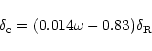
$$W_{\rm w,cor}=\left[W_{\rm w,raw} + \delta_{\rm c}\right]/(1+z)$$ (1)

(see Haynes & Giovanelli 1984). Here $W_{\rm w,raw}$ is the raw observed linewidth at w=20% or w=50% peak maximum, $z=V_{\rm HI}/c$, and $\delta_{\rm c}$ is given by

$$\delta_{\rm c}=(0.014\omega - 0.83)\delta_{\rm R}$$ (2)

where $\omega=20$ and $\omega=50$ for W₂₀ and W₅₀, respectively, and $\delta_{\rm R}$ is the velocity resolution of the measured spectrum (see Bottinelli et al. 1990). No corrections were applied for inclination angle of the source or for turbulent motions;

(4) Radial velocity, in kms^-1, corrected to the Local Standard of Rest, following the prescription of Sandage & Tammann (1981):

$$V_{\rm LSR}=V_{\rm HI}-79\cos l\cos b 296\sin l\cos b$$ +

$$36 \sin b\;\, \mbox{km\,s$^{-1}$ };$$ - (3)

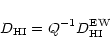
(5) Galaxy distance in Mpc, computed from $D=V_{\rm LSR}/H_{0}$;

(6) Logarithm of the H I mass in solar units, computed from the integrated line flux $S_{\rm HI}$ in Col. 8 of Table 2 and using the relation $M_{\rm HI}=2.36\;10^{5}D^{2}S_{\rm HI}$;

(7) Ratio of the ${M}_{\rm HI}$ mass to the optical B-band luminosity L_B, in solar units. L_B was derived from the mean of the absolute B magnitudes for each galaxy given in Table 6 (discussed below) and assuming a solar absolute magnitude of $M_{B,\odot}=5.48$. For NGC 7589 a B-band magnitude was taken from the NED database;

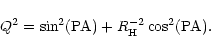
(8) Rough estimate of the H I diameter of the source in arcminutes. Estimates were made only for mapped galaxies where flux was detected at 2 or more positions (see Table 3). Following Fouqué (1984), we define the H I diameter as the isophote enclosing half of the H I mass in a flat H I disk model, which for a Gaussian H I surface density, is equal to the FWHM of the model (Fouqué 1984). Because of the elongation of the Nançay beam and the fact that our maps were obtained along an E-W axis, a correction to the raw H I diameter for the position angle and inclination of the source was also applied. Hence,

$$D_{\rm HI}=Q^{-1}D^{\rm EW}_{\rm HI}$$ (4)

where:

$$Q^{2}=\sin^{2} ({\rm PA}) + R^{-2}_{\rm H}\cos^{2} (\rm PA).$$ (5)

Here, $R_{\rm H}$ is the ratio of the major to the minor axis of the H I distribution and PA is the position angle of the major axis. We assume $R_{\rm H}=(a/b)_{\rm optical}$ and adopt the photometric position angle for PA (Fouqué 1984). Typical errors for this method of estimating $D_{\rm HI}$ are $\sim30 \pm 30$% (see Fouqué 1984).