| Issue |
A&A
Volume 698, May 2025
|
|
|---|---|---|
| Article Number | A34 | |
| Number of page(s) | 27 | |
| Section | Astrophysical processes | |
| DOI | https://doi.org/10.1051/0004-6361/202451601 | |
| Published online | 23 May 2025 | |
Light element isotopic heterogeneities in organic residues that formed by the ion irradiation of ices
1
Université Paris-Saclay, CNRS, IJCLab, 91405 Orsay, France
2
IMPMC, CNRS, MNHN-Sorbonne Université., 75005 Paris, France
3
Université Paris-Saclay, CNRS, Institut des Sciences Moléculaires d’Orsay, 91405 Orsay, France
4
Institut Curie, PSL University, Université Paris-Saclay, CNRS UAR2016, Inserm US43, Multimodal Imaging Center, Orsay, France
5
IPAG, Université Grenoble Alpes, CNRS, 38000 Grenoble, France
6
Centre de Recherche sur les Ions, les Matériaux et la Photonique CIMAP Normandie Univ, ENSICAEN, UNICAEN, CEA, CNRS, 14000 Caen, France
7
Université Paris-Saclay, CNRS, Institut de Chimie Physique, 91405 Orsay, France
⋆ Corresponding author: julien.rojas@universite-paris-saclay.fr
Received:
22
July
2024
Accepted:
22
March
2025
Context. Ultra-carbonaceous Antarctic micrometeorites (UCAMMs) are carbon-rich micrometeorites. Their organic matter formed in a N-rich environment, possibly via the galactic cosmic ray (GCR) irradiation of ice mantles at the surfaces of small bodies. Nanoscale secondary ion mass spectrometry (NanoSIMS) revealed that UCAMMs exhibit large H, C, and N isotopic heterogeneities at the micron scale.
Aims. We aim to investigate the transfer of H, C, and N isotopic heterogeneity from an ice mixture to its ion-irradiation-induced organic residue. The goal of this work is to understand the formation of H, C, and N bulk- and micron-scale isotopic heterogeneities in the organic matter of UCAMMs.
Methods. We performed irradiation experiments of isotopically heterogeneous ice films at 10 K, with swift heavy ions to model the irradiation of isotopically heterogeneous icy surfaces via GCR. The irradiated ice mixtures were subsequently annealed to room temperature, which led to the formation of refractory organic residues. NanoSIMS imagery was performed on the organic residues to identify micron-scale H, C, and N isotopic heterogeneity. The ice films consisted of N2-CH4 (9:1) and NH3-CH4 (9:1) ices that contain a thin layer of D-, 13C-, and 15N-labeled species.
Results. The irradiation-induced organic residues exhibit micron-scale isotopic anomalies. The transfer of isotopic anomalies from the ice to the organic residue appears to depend on the chemical composition of the ice film.
Conclusions. These experiments show it is possible to transfer isotopic heterogeneity that is initially present in cometary ices to refractory organic residues that formed by heavy ion irradiation. Gaseous reservoirs of volatile species with highly fractionated isotopic compositions are predicted to exist in the early Solar System and should coexist under the form of ice mantles at the surface of small bodies at large heliocentric distances. The study of organics in UCAMMs can thus shed light on the composition of N- and C-rich ices at the surface of outer Solar System small icy bodies.
Key words: astrochemistry / methods: laboratory: molecular / comets: general / Kuiper belt: general / Oort Cloud / cosmic rays
© The Authors 2025
 Open Access article, published by EDP Sciences, under the terms of the Creative Commons Attribution License (https://creativecommons.org/licenses/by/4.0), which permits unrestricted use, distribution, and reproduction in any medium, provided the original work is properly cited.
This article is published in open access under the Subscribe to Open model. Subscribe to A&A to support open access publication.
1. Introduction
Organic matter is the main carrier of carbon in interplanetary samples (Alexander et al. 2015). It is present in a diversity of objects that possibly formed and evolved in different places in the Solar System. Carbonaceous chondrites most probably originate from asteroids that formed at a variety of heliocentric distances (Hellmann et al. 2023; Levison et al. 2009; Raymond & Izidoro 2017) and further evolved in the inner Solar System. Conversely, submillimeter particles such as micrometeorites and interplanetary dust particles (IDPs) are mostly associated with cometary parent bodies (Nesvorný et al. 2011; Rojas et al. 2021) that preserved volatiles and organics from the pristine building blocks of the Solar System. Although asteroids and comets did not experience the same evolution, some of their organics may come from the same sources. The isotopic composition of H, C, and N, the main elements that constitute the organic matter, are important clues to address this question.
Over recent decades, bulk and high spatial resolution mass spectrometry techniques have revealed the isotopic diversity among samples and within samples, at the micron scale. In the insoluble organic matter (IOM) of carbonaceous chondrites, both the bulk D/H and 15N/14N ratios1 span a wide range of variation. Bulk δD ranges from −160‰ to about 3300‰ (Alexander et al. 2007). In IOM from CR chondrites (Busemann et al. 2006), local D enrichment (hotspots) can reach up to δD ≈ 20 000‰ over micron-scale regions. Similarly, bulk 15N/14N ratios in IOM are highly variable; they range from −40‰ in oxidized and reduced CV chondrites, up to 400‰ in Bells (Alexander et al. 2007), with local hot and cold spots ranging from −400‰ to 2500‰ in CR, CM, CI, and CO chondrites (Nittler et al. 2018; De Gregorio et al. 2013; Floss et al. 2014; Vollmer et al. 2020). Large variations in D/H and 15N/14N ratios are reported in IDPs (Messenger 2000; Floss et al. 2006, 2010; Busemann et al. 2006; Davidson et al. 2012; Aléon et al. 2001, 2003) and ultra-carbonaceous Antarctic micrometeorites (UCAMMs), the latter having extreme D enrichment at a local scale (δD ≈ 30000 ‰ in Duprat et al. 2010). Unlike in IOM, substantial bulk 15N-depletions are observed in UCAMMs and some C-rich IDPs (Floss et al. 2006; Davidson et al. 2012; Rojas et al. 2024), down to δ15 N ≈ ≈ − 190 ‰.
High abundances of D and 15N hotspots in organic matter are often associated with the pristine nature of their carrier phase that can be affected by chemical exchange processes or even erased by secondary processes, such as aqueous alteration and heating, which happen in the parent body. While the moderate negative δ15N values reported in the IOM of oxidized and reduced CV chondrites may be linked to secondary processing (Alexander et al. 2007), such processing is unlikely to be responsible for the 15N-depletion of the bulk OM reported in several UCAMMs and IDPs (Floss et al. 2006; Rojas et al. 2024), as they do not exhibit evidence of heating episodes or extensive aqueous alteration (Dobrică et al. 2012; Yabuta et al. 2017). Dartois et al. (2018, 2013) point out that the extreme C abundance and high N/C of UCAMMs can be explained by the formation of their OM in a N-rich environment, possibly at the surface of a small icy body. Augé et al. (2016) show that poly-HCN-like residues formed from the annealing of a N2-CH4 ice film irradiated by swift ions have an infrared (IR) signature similar to that reported in the organic matter of UCAMMs. This supports the hypothesis that the latter are likely to be formed in a cold environment where hyper-volatile ices are condensed and irradiated by galactic cosmic rays (GCR). However, the extreme isotopic variability reported in UCAMMs cannot result from isotope-selective fractionation induced by the irradiation, as demonstrated by Augé et al. (2019). It may rather originate from the initial isotopic heterogeneity of the ice at the surface of UCAMMs’ parent bodies. Theoretical derivation and chemical network models predict that volatile species can be highly fractionated during the early evolutionary stages of the Solar System (Ceccarelli et al. 2014; Aikawa et al. 2012; Visser et al. 2018). The formation of organic matter via the irradiation of condensed fractionated volatile ices may then preserve and transfer those isotopic anomalies to the induced macromolecular organics.
Numerous authors have studied the formation of organic residues (ORs) by processing volatile ices, which are of interest when tracing the evolution of interstellar medium dense clouds and (young) Solar System icy bodies, with UV, electrons, and protons (Muñoz Caro & Schutte 2003; Gerakines et al. 2004; Tachibana et al. 2017; Piani et al. 2017; Laurent et al. 2014) and, more recently, swift ions (de Barros et al. 2015; Augé et al. 2016, 2019). However, the question of the formation of isotopic heterogeneities in an OR has remained largely unaddressed. Following the work by Augé et al. (2019), we investigate the transfer of H, C, and N isotopic heterogeneity from an ice to its ion-irradiation-induced OR to shed light on the origin of isotopic heterogeneities in extraterrestrial organic matter. This study is of particular interest for understanding the origin of UCAMMs that possibly formed in an environment where the GCR flux represents an important source of energy deposition.
We performed a series of irradiation experiments of swift ions acting upon volatile ice films (IF) at 10 K, using various well-defined heterogeneous H, C, and N isotopic compositions. Organic residues formed by irradiation were analyzed with ex-situ techniques to derive their H, C, and N isotopic compositions at the submicron scale. We varied the chemical composition of the IFs to study the impact of this variation on the ORs’ formation and on the transfer of their isotopic signatures. In these experiments, the structure and composition of the IFs represent an ideal case that is not necessarily representative of the isotopic stratification of actual icy body subsurfaces. Still, the study of ORs obtained from such ice mixtures allows us to derive informative trends of what can be expected in the presence of highly fractionated ice mantles.
2. Material and methods
2.1. Experimental set-up
The experiments to look into the ion irradiation of ices were conducted at the Grand Accélerateur National d’Ion Lourd (GANIL, Caen, France) during three experimental campaigns in 2019, 2020, and 2021. We used the IGLIAS (French acronym for “Irradiation of astrophysical ices”) experimental setup (Augé et al. 2018) connected to the IRRSUD beam line to irradiate IFs with 58Ni9+ (33 MeV), 136Xe19+ (75 MeV), and 86Kr15+ (74 MeV). The IGLIAS setup consists of an ultra-high vacuum chamber able to reach a pressure of 2 × 10⁻¹⁰ mbar at a temperature of 9 K, as described by Augé et al. (2019). Three substrate windows were placed on a rotary head and cooled down to 9 K with a helium cryostat. The temperature of the head can be adjusted between 9 and 300 K with an electrical heating system. Ice films were formed by gas condensation on the cryocooled windows. During the irradiation, the window’s surface was normal to the ion beam and in-situ transmission infrared spectra were recorded with a 12° incidence angle with a Fourier transform infrared (FTIR) spectrometer (red features in Fig. 1). A quadrupolar mass spectrometer (QMS) was used to monitor the gas phase in the vacuum chamber during the gas deposition and the irradiation of the samples (green box in Fig. 1).
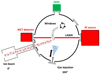 |
Fig. 1. Technical scheme of the IGLIAS chamber adapted from Augé et al. (2019). Experimental windows are disposed on a rotary head at the center of the chamber and in contact with a helium cryostat cooling system and a heating system. Ice samples are formed by the condensation of gas injected on the cooled windows. The chamber is connected to the IRRSUD ion beam at GANIL. The evolution of the IF during irradiation is monitored by a Fourier transform infrared spectrometer (FTIR) with a 12° incidence angle. A quadrupolar mass spectrometer (QMS) is connected to the chamber to monitor the gas phase. |
Zinc selenide (ZnSe) windows were used in the first experimental session. Silicon windows were used for the next sessions, which enabled infrared spectroscopy and provided better analytical conditions for the secondary ion mass spectrometry measurements (see Sect. 2.5).
2.2. Formation and composition of ice samples
We chose the chemical compositions of the ices to mimic mixes of N-, C-, and H-bearing species, which are expected to be abundant at the surface of icy bodies in the outer Solar system (Brown et al. 2011a,b; Grundy et al. 2016, 2024; Parhi & Prialnik 2023; Glein 2023; Emery et al. 2024). Either molecular nitrogen or ammonia were mixed with a small fraction of methane, the latter playing the role of the carbon provider for the OR. Two main chemical compositions were explored:
-
N2 ice mixed with 10% of CH4: N2-CH4 (9:1)
-
NH3 ice mixed with 10% of CH4: NH3-CH4 (9:1).
In the IFs, we incorporated a 15N-, 13C-, or D- labeled ice layer. The chemical compositions of the labeled layer were chosen to be similar to the compositions of the main IF, for example, 15N2-12CD4 (89:11) and 15ND3-13CH4 (89:11). However, we introduced slight variations in its composition to observe the impact of the initial ice composition on the formation of isotopic heterogeneities. The composition of the main and labeled ice layers are detailed in Table A.1. Labeled layers accounted for 1.1% up to 4.2% of the total IFs. Individual multilayered IFs were formed sequentially (steps (1)–(3) in Fig. 2) by first depositing an unlabeled ice layer, followed by a labeled ice layer, and then ending with a second unlabeled ice layer on top of it. We derived the thickness of the IFs from interference fringes in the IR spectra caused by the Fabry-Perot effect (Domingo et al. 2007) as detailed in Appendix B. The IFs were subsequently irradiated by heavy ions, which induced the production of new chemical species by radiolysis and recombination (Fig. 2, step (4)). The evolution of the ice under irradiation was monitored in-situ with the FTIR spectrometer. The processing of the ice was observed through the apparition of infrared features associated with newly formed species in the ice. During an experimental session, three IFs were deposited and subsequently irradiated on each of the three substrate windows. At the end of the irradiation, the three IFs were slowly annealed to room temperature with a gentle 0.1–0.5 K/min temperature ramp, which led to the sublimation of the remaining volatile species and the formation of refractory ORs on the windows (steps (5)–(7) in Fig. 2). The windows with the resulting ORs were extracted from the IGLIAS chamber and placed in sealed vacuum containers for transportation. In the following, the IFs are referred to as IF (IF1, IF2, …) and the organic residues as OR (OR1, OR2, …).
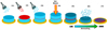 |
Fig. 2. Schematic view of the experimental protocol. The IFs are condensed by injection of a gas mixture on a substrate window at 10 K. A first isotopically unlabeled ice layer is deposited (light blue, (1)), followed by a thin layer of isotopically labled ice (red, (2)) and a final unlabeled ice layer (light blue, (3)). The whole IF is irradiated by heavy ions (4), resulting in the radiolysis of initial species and the formation of new molecules (5). At the end of the irradiation, the IF is slowly annealed from 10 K to 300 K, causing the sublimation of remaining volatile species (6) and the formation of a refractory OR (7). |
2.3. Energy deposition
We used the SRIM software (Ziegler et al. 2010) to compute the energy deposited by ions in the targets, per unit of distance, which is the stopping power S. The solid lines in Fig. 3 show the evolution of the stopping power with the depth, for a 14N2-12CH4 (9:1) IF target. To ensure energy deposition in the entire volume of the ice samples and maximize the electronic stopping power (responsible for the radiolysis of the ice) over the nuclear stopping power (Sn/Se ≪ 1, as relevant to model the GCR), we adjusted the thicknesses of the IFs (filled circles in Fig. 3) to the properties of each ion beam. Under these conditions, the stopping power can be written as
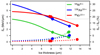 |
Fig. 3. Stopping power of ions in the ice films. Left axis and solid lines: Evolution of the electronic stopping power of ions used in the experimental sessions as a function of their penetration depth in a 14N2-12CH4 (9:1) IF, modeled with the SRIM code. Right axis and dashed lines: evolution of the nuclear over electronic stopping powers ratio as function of the penetration depths in the IFs. Filled circles indicate the size of the IFs irradiated during the experiments. |
The Sn/Se ratios, indicated by dashed lines in Fig. 3 (right axis), remained below 0.1 for each of the nine experiments.
We determined the dose, D, of energy deposited per molecule by
with the terms having the following meanings:
-
ϕt fluence measured during the irradiation (cm−2)
-
〈S〉 mean stopping power derived by integrating the stopping power along the IF depth (MeV⋅μm−1)
-
M molar mass of the target (g⋅mol−1)
-
ρ density of the ice at 10 K (g⋅ cm−3)
-
NA Avogadro constant (mol−1).
The densities of N2 and NH3 measured by Satorre et al. (2008, 2013) (ρN2 = 0.94 g⋅cm−3 at 10 K and ρNH3 = 0.67 g⋅cm−3 at 13 K) were adopted for N2-CH4 (9:1) and NH3-CH4 (9:1) ices as N2 and NH3 dominate the deposited ice mixture. Fluences were adjusted to reach doses, D, ranging from 8 to 25 eV.molecule−1, which is consistent with significant processing of the IFs that leads to the formation of ORs after annealing (Augé et al. 2016, 2019).
2.4. Quadrupolar mass spectrometer
A microvision2 mks quadrupole mass spectrometer was used to monitor the gas phase throughout the duration of the experiments. The electron impact energy was set to 70 eV and the instrument continuously scanned the range of mass-to-charge ratios, m/z, from 1 to 70, in cycles of 13 seconds. Upon impact with the electrons, a species X breaks following a fragmentation pattern. The fragmentation patterns f(X, m/z) of chemical species were self-calibrated based on the patterns that were observed for the deposition of IFs with pure compositions or made of a simple mix of two species, during the experiments presented here or the sputtering experiments that happened during the same experimental sessions (Dartois et al. 2020a,b, 2023):
with I(m/zmax) being the signal of the more intense m/z of the fragments. The labeled species (i.e., 15N2, CD4, 13CH4, 13CO, …) were assumed to behave similarly to non-labeled species (i.e., N2, CH4, CO, …) and their fragmentation patterns were extrapolated via the corresponding m/z ratios.
The QMS was used to measure the relative abundances of the constituents of the ice layers. For the labeled layers, between five and ten scans were targeted, corresponding to one to two minutes. The resulting mass spectra Iexp(m/z) were then numerically modeled by the linear combination of the fragmentation patterns of the species contributing to the signal. The modeled intensity at a given m/z was given by the sum of the contributions imodel(Xj, m/z) of the species Xj to this m/z:

where α(Xj) is a scaling factor related to the abundance of the species Xj. The estimated contribution of the species Xj to a given m/z is derived from the relative contribution of Xj and the experimental intensity:
For two species, X and Y, with the total electron-impact ionization cross sections, σimpact(X) and σimpact(Y), the abundance ratio is
![$$ \begin{aligned} \frac{[X]}{[Y]} = \frac{\sum \limits _{X_{\rm fragments}} i_{\rm estim}(X, m/z)}{\sum \limits _{Y_{\rm fragments}} i_{\rm estim}(Y, m/z)} \cdot \frac{\sigma _{\rm impact}(Y)}{\sigma _{\rm impact}(X)} \cdot \end{aligned} $$](/articles/aa/full_html/2025/06/aa51601-24/aa51601-24-eq6.gif)
The total electron-impact ionization cross sections at 70 eV were retrieved from the NIST database for N2 (2.508 Å), CH4 (3.524 Å), CO (2.516 Å), and NH3 (3.036 Å) and extrapolated for their isotopologues.
2.5. NanoSIMS
Using the NanoSIMS-50 ion probe, we analyzed the spatial distribution of D/H, 13C/12C, and 15N/14N heterogeneities in the ORs, at a sub-micron scale, by means of secondary ion mass spectrometry during four sessions at the Institut Curie (Orsay, France). The ORs were gold-coated to ensure the evacuation of charges under the primary ion beam. The insulating nature of the ZnSe windows used during the 2019 experiments prevented an efficient evacuation of charges, which led to a premature end of the analyses. The conductivity of the samples was highly improved in the following 2020 and 2021 campaigns by the use of silicon windows.
The NanoSIMS-50 ion probe was set in multicollection mode to acquire simultaneously 12CH−, 12CD−, 12C14N−, 12C15N−, and 13C14N− secondary ion maps with a 3.5–8 pA primary Cs+ ion beam. Multistack images were acquired with the same magnetic field and using the peak switching mode on the fourth electron multiplier, at mass 27, to alternatively acquire 12C15N− and 13C14N− ion maps. As a result, the number of 12C15N− and 13C14N− images in an acquisition, and their resulting total statistics, are two times lower than that of the 12CH−, 12CD−, and 12C14N− images. The acquisitions lasted between 3.5 and 14 hours, which allowed us to accumulate from 300 to 2000 consecutive plans per acquisition for 12CH−, 12CD−, and 12C14N− and from 150 to 1000 plans for 12C15N− and 13C14N−. In order to reach the mass resolution necessary to isolate the 12CD− peak from the 12CH2− interference and the 13C14N− peak from the 11B16O− interference, we worked with the high mass resolution (HMR) settings (Slodzian et al. 2014, 2017). This setup allows us to derive spatially correlated D/H, 13C/12C, and 15N/14N maps from one acquisition, using the same magnetic field.
Images of the residues, recorded by the optical camera of the NanoSIMS, are displayed in Fig. C.1 and were used to determine areas of interest. The size and definition of the analyzed surface were adapted from one residue to another based on the size of the residues’ structure, ranging from 20 × 20 μm2 (256 × 256 pixels) to 100 × 100 μm2 (308 × 308 pixels), as detailed in the Table D.1.
Raw stack images were pre-processed with the OpenMIMS plug-in (NIH/NIBIB National Resource) of the ImageJ software (Schneider et al. 2012). A drift correction was applied to the ion images of a single stack with the TomoJ plug-in (MessaoudiI et al. 2007) followed by a correction of the dead time and quasi-simultaneous arrivals effect (QSA, Slodzian et al. 2004). Advanced data treatments were performed with dedicated in-house Python routines. We derived the spatial isotopic heterogneities within the residues from hexagonal regions of interest (ROI) tiled across the ion emission images. For two given isotopes (e.g., H, D or 12C, 13C, or 14N, 15N), the isotopic ratio, Ri, associated to a hexagonal ROI, i, is given by the ratio of the sum of the counts per pixel in the ion emission images (e.g., 12CH−, 12CD− or 12C14N−, 13C14N− or 12C14N−, 12C15N−):
Assuming that the ion counts obey a Poisson statistic, the error, σRi, on the isotopic ratio, Ri, is given by
We performed several acquisitions in different locations of the residues to assess the isotopic heterogeneity at both the scale of a NanoSIMS acquisition (≈10–30 μm) and at a larger scale (≈100 μm): one acquisition on OR6, two on OR4, OR5, and OR8 and four on OR7.
3. Results
3.1. Characterization of the organic residues
The evolution of the IFs under the ion beam is visible with the IR spectra acquired during the irradiations (see Fig. E.1). It is evidenced by the decrease of features associated with the initial ice mixtures and the onset and growth of complex bands related to new chemical species formation, as described by Augé et al. (2016, 2019) and references therein.
During the annealing process, the progressive sublimation of the volatile species was monitored in IR on one target per session. Sublimated species were simultaneously recorded by the QMS. However, during this phase, the QMS was monitoring all the species sublimating simultaneously from the three irradiated IFs present in the chamber, which prevented an unambiguous association between the evolution of the IR and QMS spectra.
At the end of the annealing, IR spectra of each of the individual ORs were acquired prior to extraction from the chamber. Additional IR spectra were acquired on samples OR5, OR7, and OR8 with a FTIR microscope spectrometer (μ-FTIR). The general visual aspect of the residues is shown by the close-up images of residues OR1, OR3, OR4, OR5, OR7, and OR8 that were acquired with the μ-FTIR (Fig. 4) and the NanoSIMS-integrated camera (Fig. C).
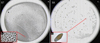 |
Fig. 4. Mosaic of optical images of the residues OR7 (a.) and OR8 (c.), formed on Silicon windows during the 2021 session. Images (b.) and (d.) are close-up images. Residue OR7 and OR8 were formed during the same session from N2-CH4 and a NH3-CH4 ice mixtures, respectively. The different structures of the residues are most probably due to the different chemical composition of the starting ice (see text). |
3.1.1. Residues of N2-CH4-dominated ices
Residues formed from IFs dominated by a 14N2-12CH4 composition display similar IR spectra, with bands at 1350 cm−1 (C-N), 1500–1650 cm−1 (C=N/C=C), 2200 cm−1 (C≡N/N≡C), 3000 cm−1 (CH2/CH3), and 2600–3500 cm−1 (NH2/NH) (OR3, OR5, OR7, and Auge 2019 in Fig. 5), which indicates the reproducibility of the IR signature of the residues. Although the aspect of the residues varied from one session to another, as shown in Fig. C, they were all equally distributed across the surface of the windows. In the 2019 session, OR1, OR2, and OR3 were made of micron-scale patches surrounded by furrows with lower quantities of matter. The residues formed during the 2020 session, OR4, OR5, and OR6, present larger flat patches of about 30 μm in size, separated by 5–10 μm-large cracks with limited amounts of matter. Noticeably, OR4 displays an empty circular zone, surrounded by smaller patches (see Fig. C). Residue OR7, formed during the 2021 session from a N2-CH4 IF, is made of 30 μm-large patches distributed uniformly on the substrate window surface (Figs. 4, a and b.). The thicknesses of OR2, OR4, and OR7 were measured by atomic force microscope (AFM) as detailed in Appendix F.
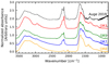 |
Fig. 5. IR spectra of OR3, OR5, OR7, and OR8. The spectrum of the OR reported by Augé et al. (2019) is reported with a dashed black line. |
3.1.2. Residues of NH3-CH4-dominated ices
Residues OR8 and OR9 were formed during the 2021 session by the irradiation of a 14NH3-12CH4 ice mixture. The IR spectrum of OR8 displays a lower C≡N band and a slightly enhanced C-N band compared to the C=N, C=C, and N-H bands. Strikingly, a C-D stretch feature is observed at 2030 cm−1. This feature was previously reported in an OR formed by the irradiation of 18.5 μm-thick 14N2-12CH4 IF with a 0.1 μm-thick pure CD4 layer (dotted black line in Fig. 5, Augé et al. 2019) and attests to the fact that a significant amount of the deuterium atoms initially present in the labeled layer of the IF was transferred to the OR. Residues OR8 and OR9 differ from the other residues by their aspect, with most of the material concentrated in 100–200 μm-large and several-microns-thick droplets (Figs. 4, c. and d.) as shown by the height data in Appendix F.
Since residues OR7, OR8, and OR9 were synthesized during the same experimental session (i.e., processed with similar doses deposited by the same ions, experiencing the same temperature ramp), their differences most probably result from the chemical properties of their respective initial ices.
3.2. Composition of the ice films
The composition of the IFs inferred from QMS-derived data and partial pressure data are listed in the fourth and fifth row of Table A.1 in roman and italic script, respectively. For IF4, IF5, IF7, and the unlabeled layers of IF6, the compositions were determined with the QMS. For IF8 and the labeled layer of IF6 (made of a NH3-CH4 mixture), the compositions were given by the partial pressures measured in the mixing chamber, given the complexity of the QMS spectra. The compositions of IF4, IF5, IF6, IF7, and IF8 are N2-CH4 (74:26)/15N2-13CD4 (85:15), N2-CH4 (79:21)/15N2-13CO (82:18), N2-CH4 (81:19)/15NH3-13CH4 (1:1), N2-CH4 (88:12)/15N2-13CD4-13CO (78:12:10), and NH3-CH4 (89:11)/15NH3-13CH4 (89:11), respectively. Yet, it is important to note that the QMS probes the gas phase in which the relative abundances of species may differ from what actually constitutes the IF.
3.3. NanoSIMS analyses
NanoSIMS maps were acquired in different locations of the residues to assess the isotopic variability at different scales. The results of the NanoSIMS analyses are displayed in Fig. 6 with OR4 (two analyses) in blue, OR5 (two analyses) in amber, OR6 in pink (one analysis), OR7 (four analyses) in red, and OR8 (two analyses) in green. Panels a and b show the 15N/14N distribution against the 13C/12C and the D/H distributions, respectively. The sample OR5 is not reported in panel b since it was made without a D labeling. To highlight the intrinsic variation of the isotopic compositions at the scale of individual NanoSIMS images (i.e., independent from the initial relative amount of the labeled component in the OR), normalized isotopic maps of residues OR4, OR5, OR6, OR7, and OR8 are displayed in Fig. 7 and in Appendix G.
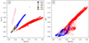 |
Fig. 6. Graphs of the distribution of isotopic values measured in the residues OR4 (blue), OR5 (orange), OR6 (pink), OR7 (red), and OR8 (green). (a): 15N/14N against 13C/12C. (b): 15N/14N against D/H. Residues OR4, OR5, and OR6 were formed during the 2020 session and residues OR7 and OR8 during the 2021 session. Residues formed during the same session experienced the same conditions, that is, they formed on the same substrate, irradiated with the same ions, and experienced the same annealing. |
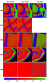 |
Fig. 7. Ratio images derived from the NanoSIMS acquisitions. The color scale shows the relative variations of the isotopic composition from the mean value of the individual images. Left column: Relative 15N/14N. Center column: Relative 13C/12C; relative D/H. Images of residues OR4, OR5, OR6, OR7, and OR8 are shown in rows one, two, three, four, and five, respectively. No D/H image is shown for OR5 since no D-rich layer was added to the initial IF. The white scale bar is 5 μm. |
As shown in Fig. 6, the distributions of isotopic ratios in OR4, OR5, OR6, and OR7 follow fractionation lines that derive from the mixing of the two different isotopic compositions. The spreading of the isotopic ratios along these lines derives from the extent of mixing experienced by the samples during the formation process.
Most of the surface of OR4 and OR5 presents a limited heterogeneity. However, OR4 presents highly heterogeneous 15N/14N, 13C/12C, and D/H in the matter surrounding the empty circular zones (Fig. 7 and Fig. C.1). The 15N-, 13C-, and D-rich component (green in Fig. 7) is localized in 10 μm-large patches while the 15N-, 13C- and D-poor component (blue in Fig. 7) appears in narrow regions surrounding bigger patches of matter that have the mean isotopic composition (red in Fig. 7). However, as shown in Fig. 6, the composition of some zones of OR4 falls out of the 13C/12C versus D/H and 15N/14N versus D/H lines and forms a “coma-shaped” secondary trend.
Residue OR7 presents large isotopic heterogeneities that are not bound to specific regions, unlike OR4. These isotopic variations correlate with the distribution of matter within organic droplets (Fig. 7), which indicates that the formation of the residue to a large extent preserved the memory of the two components initially present in the ice mixture. Contrarily, OR8, which formed during the same session, displays a more homogeneous composition possibly due to a more extensive mixing of the two components initially present in the IF. While for OR8 the 13C/12C versus 15N/14N distribution (Fig. 6a) has a positive slope, the D/H versus 15N/14N distribution is flat. Similarly to OR4, some zones in OR7 have isotopic compositions that do not follow the main fractionation lines (Fig. 6b).
4. Discussion
4.1. Origin of the isotopic composition
The labeling of heavy isotopes (D, 13C, 15N) was achieved by incorporating isotopically labeled species in the IFs. The bulk isotopic compositions of the samples (IFs and ORs) range from 0.01 to 0.04 (Table A.1). As shown by Augé et al. (2019) in an organic residue obtained by the irradiation of an unlabeled N2-CH4 ice mixture, the isotope-selective fractionation induced by irradiation can lead to a fractionation of at most a few hundred permil, which is an increase of the D/H ratio of about 1⋅10−4, which is, at least, two orders of magnitude lower than the fractionation observed in the experiments reported here. Thus, the isotopic compositions and heterogeneities of the ORs reported here are due to the mixing of precursors that arises from the labeled and unlabeled components in the original IFs. The fact that the irradiation-induced fractionation is negligible is supported by the absence of D/H variations with 13C/12C and 15N/14N in OR5 (Figs. H.1, a-2 and a-3) that was formed without D labeling.
4.2. Two components mixing
Ice films were made of layers with two distinct isotopic compositions forming two isotopic poles. An isotopic pole was characterized by its relative abundances of N, C, H, and O atoms and its isotopic ratios RN, RC, and RH. The ratio RO was not considered in this study as no oxygenated molecules were incorporated in the unlabeled ice layers. Isotopic ratios can be converted into purity factors pN, pC, pH, such as pX = RX/(RX + 1). In the absence of irradiation-induced fractionation, the mixing of these two poles, for an element X with two isotopes AX and A + 1X, should obey to a mixing equation of general form

with the terms having the following meanings:
-
c,c′ relative abundances of the element X in the two poles;
-
αX mixing coefficient, that is, the fraction of the labeled pole in the mix, for the element X.
We derived the relative abundances c and c′ of N, C, and H from the relative abundances of N2, CH4, and CO and their isotopologues measured with the QMS for IF4, IF5, IF6, and IF7 (Table A.1). For IFs containing NH3 or 15ND3 (i.e., IF8 and the labeled layer of IF6), we used the partial pressure to derive their relative abundances. The unlabeled ices were assumed to have D/H, 13C/12C, and 15N/14N ratios equal to the standard values, VSMOW, VPDB, and AIR, respectively.
Equation (9) defines fractionation lines for H, C, and N as a functions of αH, αC, αN and the relative abundances of H, C, and N in the two poles: c and c′. Fractionation lines derived from the model for varying abundances c′ and αH, αC, αN are displayed with dotted lines in Figs. 8, H.1, H.2, H.3, and H.4. In the following sections, we discuss the role of parameters αX and c′ in the behavior of the fractionation lines. We considered that the relative abundances c in the unlabeled ice layers are fixed since variations of parameters c and c′ have comparable impacts on the behavior of fractionation lines.
4.2.1. Case αN = αC = αH = α
At the first order, one can assume that H, C, and N have the same mixing efficiencies during the synthesis process (αN/αC ≈ 1, αN/αH ≈ 1, αC/αH ≈ 1). The fractionation lines should then be dominated by the IF relative elemental abundances. This case is illustrated in row a of Figs. 8, H.1, H.3, and H.4 and rows a, b, and c of H.2, where fractionation lines derived from the abundances determined with the QMS or the partial pressure are shown with bold dashed black lines. Fractionation lines with a range of possible composition are displayed with thin dashed lines. The fraction of mixing of the two poles, α = αN = αC = αH, is indicated with blue-red color levels. The fractionation lines are unaffected by variations in abundance when isotopes of two different elements are carried by the same molecule, as, for example, D and 13C in 15N2-13CD4 (Fig. 8, a-3) and D and 15N in 15ND3-13CH4 (Fig. H.3, a-2). Within this assumption, the slopes of the mixing lines are set by the chemical composition of the IF at their formation, before irradiation (steps 1–3 of Fig. 2).
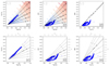 |
Fig. 8. Comparison of the NanoSIMS data on OR4 (filled circles) and the IF4 mixing lines derived from the mixing model. Columns 1, 2, and 3 show the 15N/14N versus 13C/12C, 15N/14N versus D/H, and 13C/12C versus D/H compositions, respectively. Row a: mixing lines for αN = αC = αH = α. The value of α is indicated by the blue to red color contours. IF mixing lines with varying labeled layer compositions are displayed with dashed lines. The composition of the unlabeled ice is indicated in gray. Row b: the composition of IF4 is fixed and the mixing factors αN, αC, αH are free parameters. The value of the mixing factors are given by the gray scale on the top and right axes. The nominal mixing lines are plotted with bold dotted lines. |
4.2.2. Case αN ≠ αC, αN ≠ αH and αC ≠ αH
Assuming different mixing coefficients αN, αC, αH and fixed IF relative abundances c′ (see Sect. 3.2), the behavior of the fractionation lines is driven by the relative difference between the mixing coefficients, that is, the efficiency of mixing of H, C, and N, as shown in row b of Figs. 8, H.1, H.3, and H.4 and row d of H.2. Mixing coefficients are indicated in gray in the top and right axes. Lines with constant αN/αC, αN/αH and αC/αH are plotted with dashed lines. The slopes of the fractionation lines are driven by the relative difference between the mixing factors, which reflects the efficiency of mixing of the elements during the OR formation (i.e., irradiation and annealing, steps 4–7 of Fig. 2). Contrarily to the previous case, the initial chemical composition of the IF has a limited impact on the behavior of the mixing lines. Importantly, the efficiency of incorporation of elements from the IF to the OR has also to be considered. However, variations in incorporation efficiency are indiscernible from variations in mixing efficiency, since, for instance, a low α can be caused by an extensive mixing of the labeled and unlabeled poles or by an inefficient incorporation of the labeled pole in the final OR.
4.3. Comparison of the ice films and organic residues mixing lines
NanoSIMS analyses showed isotopic heterogeneity spatially distributed across the ORs, giving rise to mixing lines in the isotopic ratio plots, hereafter “OR mixing lines” (Fig. 6). Those OR mixing lines can be attributed to the mixing of the isotopically distinct irradiation-induced precursors that arise from the labeled and unlabeled components in the IFs and can be compared to the mixing lines derived from the two-components mixing model discussed in Sect. 4.2, hereafter “IF mixing lines”. The extension of the OR mixing lines can be related to the mixing coefficients αX, which indicate the amount of mixing happening during the synthesis of the OR. Eventually, if an irradiated IF is fully homogenized during the synthesis process (irradiation and annealing), the distribution of isotopic values in the OR will gather around the average bulk isotopic composition of the ice mixture and will not follow a mixing line. Two elements with a different mobility during the synthesis (Sect. 4.2.2) will lead to a change in slope of the mixing lines. In the following, we compare the isotopic compositions measured with the NanoSIMS to the two component mixing models for OR4, OR5, OR6, OR7, and OR8. The IF mixing lines with the nominal composition measured by the QMS or estimated with partial pressures (Table A.1) and verifying α = αN = αC = αH are referred to as the nominal mixing lines.
4.3.1. OR5/IF5
IF5 was made of 15N2-13CO (labeled layer) and N2-CH4 (unlabeled layers). No D-rich component was incorporated in IF5. Fig. H.1 shows the OR5 and IF5 mixing lines. As expected from the absence of D labeling in this sample, the OR mixing lines in a-2 and a-3 are horizontal, that is, the D/H composition is constant with no dependence on the 15N/14N or 13C/12C compositions. On the 13C/12C versus 15N/14N plots (a-1 and b-1), the OR mixing line is consistent with the IF mixing line of nominal composition and verifying αC/αN ≈ 0.9, which indicates that the isotopic composition of OR5 can be reproduced by a two-component mixing model with similar mixing efficiencies for C and N. The mixing coefficients alpha range from αN ≈ 0.9 − 3.0% and αC ≈ 0.8 − 2.9%.
The good agreement between the OR5 mixing line and the nominal IF5 mixing line indicates that the C and N atoms recombined locally (or had a similar mobility before recombination). However, the H atoms associated with the 13C- and 15N-rich component of the residues necessarily originate from the unlabeled ice layer as no H atoms were present in the labeled layer of IF5, thus evidencing the mobility of H atoms during the synthesis process.
4.3.2. OR4/IF4
IF4 was made of a labeled layer of 15N2-13CD4 (85:15) and unlabeled layers of N2-CH4 (74:26). Although no variation in chemical composition was introduced in IF4, the labeled layer presented a N to C excess compared to the unlabeled layers. The OR4 and IF4 mixing lines are displayed in Fig. 8. On the 13C/12C versus 15N/14N plots, a single OR mixing line is visible, which is consistent with an IF mixing line of composition 15N2-13CD4 (77:23) (a-1). Conversely, two distinct trends are visible on the D/H versus 15N/14N and D/H versus 13C/12C graphs. The first trend is a line that is consistent with the nominal IF4 mixing line in a-2 but cannot be fitted with a specific IF composition in a-3. The second trend is coma-shaped and cannot be reproduced with a simple two -component mixing model.
Linear trends in Figs. 8, a-1, a-2, a-3 are not consistent with a single chemical composition, assuming αN = αC = αH (Sect. 4.2.1), since two different chemical compositions are necessary to explain the 13C/12C versus 15N/14N and D/H versus 15N/14N OR mixing lines. Still, they can be reproduced by assuming different mixing efficiency verifying αC/αN ≈ 1.6, αH/αN ≈ 1 and αH/αC ≈ 0.7 (Sect. 4.2.2) as shown in Figs. 8, b-1, b-2, b-3. The mixing coefficients range between αN ≈ 0.8 − 8.5%, αC ≈ 0.8 − 14.5% and αH ≈ 0.0 − 7.0%.
Noticeably, in the 13C/12C versus 15N/14N plot, the IF4 mixing line in agreement with the OR4 mixing line has the composition 15N2-13CD4 (77:23), which is similar in proportion to the composition of the unlabeled layer N2-CH4 (74:26) and suggests that the excess of 15N in the labeled layer could not be incorporated in the OR. Given that C atoms constitute the backbone of the OR, the incorporation of 13C from the labeled ice layer has to be more efficient than the incorporation of 15N, leading to an apparent labeled ice composition poorer in 15N2 than expected and a αC/αN ratio greater than 1. Differently, the lower αH/αC likely reflects the higher diffusion efficiency of H atoms compared to C atoms.
The coma-shaped fractionation lines in Figs. 8b-2 and b-3 indicate that portions of the residue have low D/H associated with a wide range of 13C/12C and 15N/14N, while another portion has high 13C/12C and 15N/14N associated with a variable range of D/H. The regions of OR4 displaying these isotopic compositions are spatially located around empty circular areas where the OR forms smaller patches and furrows (Fig. 7, Fig. C.1 and Fig. G.1), which possibly indicates that the composition of the OR in these regions was modified by a local process. Local formation of 15N- and 13C-rich radicals that subsequently combined with H and D atoms may have given rise to a 15N- and 13C-rich residue with heterogeneous D/H. Regions of OR4 concerned by such processes are limited and complimentary experiments would be needed to further constrain this phenomenon.
4.3.3. OR7/IF7
The composition of the labeled layer of IF7 was 15N2-CD4-13CO (78:12:10). The unlabeled layer was made of N2-CH4. Due to the fact that the labeled layer of IF7 was made of three components, we developed three mixing models for the IF7 mixing lines. In the first model, the 15N2 abundance is fixed and the abundances of CD4 and 13CO are varying (Fig. H.2, row a); in the second model, the CD4 abundance is fixed and the abundances of 15N2 and 13CO are varying (Fig. H.2, row b); and in the third model, the 13CO abundance is fixed and the abundances of 15N2 and CD4 are varying (Fig. H.2, row c).
Two OR7 mixing trends are visible on the D/H versus 15N/14N and D/H versus 13C/12C plots (Figs. H.2, d-2, d-3). The main linear trend fits with IF mixing lines with αC/αN ≈ 0.45, αH/αN ≈ 0.6, αH/αC ≈ 1.25 and the secondary linear trend fits with IF mixing lines αC/αN ≈ 0.45, αH/αN ≈ 0.25, αH/αC ≈ 0.50 (Figs. H.2, d-1, d-2, d-3). Mixing coefficients for OR7 range from αN ≈ 3.3 − 18.4%, αC ≈ 1.2 − 8.7% and αH ≈ 0.9 − 11.2%. Importantly, the secondary mixing lines of OR7 are only formed by data points from the fourth analysis of OR7 (row 5 of Fig. G.1), while the main mixing lines reflect the composition measured in all the four analyses performed on OR7. Secondary OR7 mixing lines differ from the main mixing lines by a higher mixing efficiency of H atoms compared to N and C atoms. Thus they originate from regions where H atoms were possibly more extensively mixed or lost than C and N atoms, which highlights the existence of local variations within the organic residue.
The 13C/12C versus 15N/14N plots (a-1, b-1, c-1 in Fig. H.2) show that OR7 mixing lines are consistent with IF7 mixing lines associated with higher abundances of CD4 than 13CO. Such a trend is interpreted as being an apparent effect of the better incorporation of C atoms from CD4 than 13CO in the final organic residue caused by the more efficient radiolysis of CD4 than 13CO, as observed by Baratta et al. (2015) and might not reflect a difference in mixing efficiency. Contrarily, the D/H versus 15N/14N OR7 mixing line is likely to reflect the higher mixing efficiency of D atoms compared to 15N atoms (αH/αN ≈ 0.6). Finally, the D/H versus 13C/12C OR7 mixing line results from the low incorporation of 13C from 13CO and the high mixing efficiency of D from CD4.
4.3.4. OR8/IF8
IF8 was made of 15ND3-13CH4 and NH3-CH4. OR8 presents an extensively homogenized isotopic composition (Fig. H.3). In the 13C/12C versus 15N/14N plots, the OR mixing line is consistent with the 15ND3-13CH4 (93:7) IF mixing line (a-1). The OR mixing line in the D/H versus 15N/14N plots cannot be adjusted by varying the chemical composition of IF8 (b-1). Finally, in the D/H versus 13C/12C graphs, the OR mixing line is consistent with the 15ND3-13CH4 (78:22) IF mixing line. Therefore, OR8 mixing lines cannot be modeled by the mixing model assuming equal mixing efficiency for H, C, and N. Still, assuming different mixing efficiencies (Sect. 4.2.2), OR8 mixing lines are consistent with IF mixing lines, which verifies αC/αN ≈ 0.65, αH/αN ≈ 0.3 and αH/αC ≈ 0.5 (Figs. H.3, b-1, b-2, b-3). The values of the mixing coefficients for OR8 range from αN ≈ 2.8 − 3.3%, αC ≈ 1.8 − 2.4%, and αH ≈ 0.6 − 1.1%.
The ranges of variations of OR8 mixing coefficients indicate that the unlabeled and labeled isotopic poles were extensively mixed during the synthesis process. We speculate that the large amount of NH3 in IF8 favored the mixing by lowering the viscosity of the irradiated ice during its annealing, as observed by Tachibana et al. (2017) for UV-irradiated H2O-CH3OH-NH3 ice. Tachibana et al. (2017) and Loeffler & Baragiola (2012) reported the formation of H2 bubbles during the annealing of UV- and proton-irradiated H2O-CH3OH-NH3 and H2O-NH3 ices, mostly attributed to the dissociation of H from NH3 and CH3OH. From the properties of those bubbles, Tachibana et al. (2017) determined that the H2O-CH3OH-NH3 irradiated ice mixture was going through a liquid-like behavior, characterized by a low-viscosity, between 50 K to 65 K, which corresponds to the temperature of the phase transition from high- to low-density amorphous water ice. The authors hypothesize that this transient liquid-like state enhances the mobility of species in the irradiated ice mixture. Although IF8 did not contain H2O, its dominant NH3 component underwent a transition from its amorphous to metastable or crystalline phases (Holt et al. 2004) during annealing (Appendix H) and may have experienced a similar liquid-like state that led to the efficient mixing of the labeled and unlabeled isotopic poles.
4.3.5. OR6/IF6
IF6 combined an unlabeled layer of N2-CH4 and a labeled layer of 15ND3-13CH4. OR and IF mixing lines for OR6/IF6 are shown in Fig. H.4. The OR mixing line in the 13C/12C versus 15N/14N plot fits with the αC/αN ≈ 0.35 IF mixing line (b-1). Given their shapes, the OR mixing lines in the D/H versus 15N/14N (a-2 and b-2) and D/H versus 13C/12C (a-3 and b-3) plots cannot be reproduced with the two-component mixing model, which possibly indicates the importance of complex physicochemical mechanisms during the OR synthesis. While in the other samples the labeled and unlabeled layers have a similar chemical composition, the labeled layer of IF6, 15ND3-13CH4 (1:1), was drastically different from the unlabeled layer, N2-CH4 (81:19), with about three times more carbon, five times more hydrogen or deuterium and seven times less nitrogen.
Noticeably, OR6 has a 15N-rich composition (αN≈ 0.6–18.1%) relative to the 13C (αC≈ 1.5–6.9%) and D (αH≈ 0.0–2.2%) composition. Such enrichment in 15N can be caused by the more effective radiolysis of 15ND3 compared to that of N2, leading to a better incorporation of 15N over 14N in the OR. In parallel, the homogeneous D/H composition denotes the extensive mixing of D and H atoms, abundant in the isotopically labeled ice layer. The difference in chemical composition of the isotopically labeled and unlabeled ice layers of IF6 might have driven the isotopic composition of the resulting OR. Still, the complex nature of IF6 prevents any definitive conclusions.
4.3.6. Interpretation of the mixing lines
Comparison of the OR and IF mixing lines for OR4, OR5, OR7, and OR8 indicates that the H, C, and N isotopic heterogeneities in the ORs can be mostly explained by the mixing of the two isotopic poles initially present in the parent IFs. Differences in slopes between the OR and the nominal IF mixing lines cannot be reproduced by varying the proportions of the components within the IFs, but rather arise from the distinct incorporation and mixing efficiencies of H, C, and N during the synthesis process. However, all the samples considered are characterized by different ratios, αC/αN, αH/αN and αH/αC, which strongly suggests that the chemical composition of the IFs has a substantial impact on the mobility of H, C, and N atoms and associated radiolysis products. Noticeably, while mixing coefficients associated with OR4, 5, 6, and 7 span a range of variation of several percent, the ones associated with OR8 show very limited variations, which indicates that the two initial isotopic components within IF8 were extensively mixed during the synthesis of OR8. Compared to the other ice mixtures, the large amount of NH3 molecules in IF8 may have enhanced the mobility during the annealing, as observed with other NH3-bearing ices by Tachibana et al. (2017), and favored the mixing of H, C, and N atoms, leading to a more homogeneous isotopic composition. Finally, fractionation lines of OR6 and the secondary trend of OR4 are not consistent with the two-component mixing model of Sect. 4.2. For those cases, the fractionation might have been dominated by specific physicochemical processes that are out of the scope of this study.
These experiments show that ORs formed from the annealing of irradiated ices can keep a memory of the isotopic heterogeneities initially present in the IFs. However, the efficiency of transfer of such isotopic heterogeneities to the OR depends on the chemical composition of the IFs. While this transfer appears to be efficient for N2-CH4 IFs, it is not the case for the NH3-CH4 IF. Large abundances of NH3 in ice mixtures possibly contribute to the homogenization of the isotopic heterogenities initially present. Thus, the chemical composition of a parent ice plays a role in the formation of local-scale isotopic heterogeneity in the irradiation-induced OR.
4.4. Implications for UCAMMs
The characteristics of ORs produced in this study are compatible with the large H, C, and N isotopic heterogeneities observed in UCAMMs. The 15N-depleted signature of some UCAMMs and C-rich IDPs (Sect. 1) possibly derives from the 15N-poor primordial N2 condensed on the surface of small bodies in the outermost regions of the Solar System. Importantly, a small body with a surface temperature low enough to retain N2 ice should also retain, at the same time, less volatile ices such as NH3 or HCN (Parhi & Prialnik 2023), likely richer in 15N (Appendix J.1), possibly preventing the record of the primordial 15N/14N composition (δ15N ≈ − 380‰) in the irradiation-induced organic matter, under the effect of mixing, and inducing large N isotopic heterogeneity.
Since kilometer-sized icy objects located at heliocentric distances larger than ∼100 a.u. are likely to have hypervolatile ice mantles, one can expect a variety of chemical composition and hence, large heterogeneity of isotopic composition within their mantles. Such heterogeneity could then be transferred to their irradiation-induced organics, after irradiation by the GCR (Appendix J.2). Therefore, UCAMM-like particles originating from distinct parent bodies are not expected to have similar isotopic compositions. The observation of large D, 13C, and 15N excesses or depletion in different UCAMMs can be explained by the specific journey and history of their parent bodies, leading to the accretion of precursor ices with a variety of isotopic compositions.
5. Conclusion
We performed irradiation experiments to study the transfer of H, C, and N isotopic heterogeneities from an ice film to a refractory organic residue. We irradiated ice films with a bimodal isotopic composition, with swift heavy ions to simulate exposure to cosmic rays in the outer Solar System. After irradiation at 10 K, the slow annealing of the processed ice films led to the formation of refractory organic residues. The analysis of the organic residues by NanoSIMS revealed their micron-scale isotopic composition and we developed a two-component mixing model to interpret their H, C, and N isotopic distributions. Micron-scale isotopic heterogeneities were evidenced for organic residues synthesized from N2-CH4 ice mixtures. The large isotopic variations observed are consistent with a two-component mixing of the isotopic end members initially present in the ice films, and a negligible isotope-selective atomic loss induced by the ion irradiation. The organic residue formed from a NH3-CH4 ice mixture presents limited micron-scale heterogeneities, which shows that the radiolytic products deriving from the two initial end members in the ice mixture were more extensively mixed than in the case of N2-CH4. We hypothesize that this extensive mixing is driven by the large abundance of NH3 that favors the mobility of species during the annealing of the ice film after ion irradiation. Additional ion-irradiation experiments of NH3-rich ice mixtures would help clarify the behavior of irradiated NH3 ice during annealing and its role in the formation of isotopic heterogeneities.
The results from the present study show that irradiation by the GCR of isotopically heterogeneous N- and C-rich ice mantles at the surface of small objects in the outer part of the Solar System can explain not only the formation of the N-rich organic matter of UCAMMs with a consistent chemical composition but also the formation of micron-scale H, C, and N isotopic heterogeneities. Highly fractionated H, C, and N volatile reservoirs predicted to co-exist in the Solar System are possibly the parent reservoirs of the organic matter in UCAMMs. The organic matter in UCAMMs and C-rich IDPs can thus shed light on the isotopic and chemical properties of hypervolatile species at the surface of the most remote objects in the outer Solar System.
Acknowledgments
This work was financially supported by ANR (Project COMETOR 18-CE31-0011), Region Ile de France DIM-ACAV+ (projet C3E), CNES, CNRS INSU-PCMI, IN2P3 and Labex P2IO. (We acknowledge) the CurieCoreTech, the technological facilities within Institut Curie, for the use of Curie-NanoSIMS. The irradiation experiments were performed at the Grand Accélérateur National d’Ions Lourds (GANIL) by means of the CIRIL Interdisciplinary Platform, part of CIMAP laboratory, Caen, France. We thank the staff of CIMAP-CIRIL and GANIL for their invaluable support. We acknowledge the fundings from ANR IGLIAS grant ANR-13-BS05-0004 of the French Agence Nationale de la Recherche.
References
- Aikawa, Y., Wakelam, V., Hersant, F., Garrod, R. T., & Herbst, E. 2012, ApJ, 760, 40 [NASA ADS] [CrossRef] [Google Scholar]
- Aikawa, Y., Furuya, K., Hincelin, U., & Herbst, E. 2018, ApJ, 855, 119 [NASA ADS] [CrossRef] [Google Scholar]
- Aléon, J., Engrand, C., Robert, F., & Chaussidon, M. 2001, GCA, 65, 4399 [Google Scholar]
- Aléon, J., Robert, F., Chaussidon, M., & Marty, B. 2003, GCA, 67, 3773 [Google Scholar]
- Alexander, C. M. O., Fogel, M., Yabuta, H., & Cody, G. D. 2007, Geochim. Cosmochim. Acta, 71, 4380 [NASA ADS] [CrossRef] [Google Scholar]
- Alexander, C. M. O., Bowden, R., Fogel, M. L., & Howard, K. T. 2015, Meteor. Planet. Sci., 50, 810 [NASA ADS] [CrossRef] [Google Scholar]
- Altwegg, K., Balsiger, H., & Fuselier, S. A. 2019, ARA&A, 57, 113 [NASA ADS] [CrossRef] [Google Scholar]
- Anderson, S. E., Rousselot, P., Noyelles, B., Jehin, E., & Mousis, O. 2023, MNRAS, 524, 5182 [NASA ADS] [CrossRef] [Google Scholar]
- Arpigny, C., Jehin, E., Manfroid, J., et al. 2003, Science, 301, 1522 [CrossRef] [PubMed] [Google Scholar]
- Augé, B., Dartois, E., Engrand, C., et al. 2016, A&A, 592, A99 [NASA ADS] [CrossRef] [EDP Sciences] [Google Scholar]
- Augé, B., Been, T., Boduch, P., et al. 2018, Rev. Sci. Instrum., 89, 075105 [Google Scholar]
- Augé, B., Dartois, E., Duprat, J., et al. 2019, A&A, 627, A122 [NASA ADS] [CrossRef] [EDP Sciences] [Google Scholar]
- Baratta, G. A., Chaput, D., Cottin, H., et al. 2015, Planet. Space Sci., 118, 211 [NASA ADS] [CrossRef] [Google Scholar]
- Bennett, C. J., & Kaiser, R. I. 2007, ApJ, 660, 1289 [NASA ADS] [CrossRef] [Google Scholar]
- Biver, N., Moreno, R., Bockelée-Morvan, D., et al. 2016, A&A, 589, A78 [NASA ADS] [CrossRef] [EDP Sciences] [Google Scholar]
- Biver, N., Bockelée-Morvan, D., Paubert, G., et al. 2018, A&A, 619, A127 [NASA ADS] [CrossRef] [EDP Sciences] [Google Scholar]
- Bockelée-Morvan, D., Biver, N., Jehin, E., et al. 2008, ApJ, 679, L49 [CrossRef] [Google Scholar]
- Bockelée-Morvan, D., Calmonte, U., Charnley, S., et al. 2015, Space Sci. Rev., 197, 47 [Google Scholar]
- Bottger, G. L., & Eggers, D. F., Jr. 1964, J. Chem. Phys., 40, 2010 [Google Scholar]
- Bouilloud, M., Fray, N., Bénilan, Y., et al. 2015, MNRAS, 451, 2145 [Google Scholar]
- Brown, M. E., Burgasser, A. J., & Fraser, W. C. 2011a, ApJ, 738, L26 [NASA ADS] [CrossRef] [Google Scholar]
- Brown, M. E., Schaller, E. L., & Fraser, W. C. 2011b, ApJ, 739, L60 [NASA ADS] [CrossRef] [Google Scholar]
- Burgdorf, M., Cruikshank, D. P., Dalle Ore, C. M., et al. 2010, ApJ, 718, L53 [Google Scholar]
- Busemann, H., Young, A. F., Alexander, C. M. O., et al. 2006, Science, 312, 727 [NASA ADS] [CrossRef] [Google Scholar]
- Calvani, P., Lupi, S., & Maselli, P. 1989, J. Chem. Phys., 91, 6737 [Google Scholar]
- Ceccarelli, C., Caselli, P., Bockelée-Morvan, D., et al. 2014, in Protostars and Planets VI, eds. H. Beuther, R. S. Klessen, C. P. Dullemond, & T. Henning, 859 [Google Scholar]
- Cooper, J. F., Christian, E. R., Richardson, J. D., & Wang, C. 2003, Earth Moon Planets, 92, 261 [NASA ADS] [CrossRef] [Google Scholar]
- Dartois, E., Engrand, C., Brunetto, R., et al. 2013, Icarus, 224, 243 [NASA ADS] [CrossRef] [Google Scholar]
- Dartois, E., Engrand, C., Duprat, J., et al. 2018, A&A, 609, A65 [NASA ADS] [CrossRef] [EDP Sciences] [Google Scholar]
- Dartois, E., Chabot, M., Bacmann, A., et al. 2020a, A&A, 634, A103 [NASA ADS] [CrossRef] [EDP Sciences] [Google Scholar]
- Dartois, E., Chabot, M., Id Barkach, T., et al. 2020b, Nucl. Instrum. Methods Phys. Res. B, 485, 13 [Google Scholar]
- Dartois, E., Chabot, M., da Costa, C. A. P., et al. 2023, A&A, 671, A156 [NASA ADS] [CrossRef] [EDP Sciences] [Google Scholar]
- Davidson, J., Busemann, H., & Franchi, I. A. 2012, Meteor. Planet. Sci., 47, 1748 [Google Scholar]
- de Barros, A. L. F., da Silveira, E. F., Bergantini, A., Rothard, H., & Boduch, P. 2015, ApJ, 810, 156 [Google Scholar]
- De Gregorio, B. T., Stroud, R. M., Nittler, L. R., et al. 2013, Meteor. Planet. Sci., 48, 904 [NASA ADS] [CrossRef] [Google Scholar]
- De Prá, M. N., Hénault, E., Pinilla-Alonso, N., et al. 2024, Nat. Astron., 9, 252 [Google Scholar]
- D’Hendecourt, L. B., & Allamandola, L. J. 1986, A&A, 64, 453 [Google Scholar]
- Dobrică, E., Engrand, C., Leroux, H., Rouzaud, J.-N., & Duprat, J. 2012, Geochim. Cosmochim. Acta, 76, 68 [CrossRef] [Google Scholar]
- Domingo, M., Millán, C., Satorre, M. A., & Cantó, J. 2007, in Optical Measurement Systems for Industrial Inspection V, eds. W. Osten, C. Gorecki, & E. L. Novak, SPIE Conf. Ser., 6616, 66164A [Google Scholar]
- Donn, B. 1976, NASA Special Publication, 393, 611 [Google Scholar]
- Duprat, J., Dobrică, E., Engrand, C., et al. 2010, Science, 328, 742 [NASA ADS] [CrossRef] [Google Scholar]
- Emery, J., Wong, I., Brunetto, R., et al. 2024, Icarus, 414, 116017 [NASA ADS] [CrossRef] [Google Scholar]
- Füri, E., & Marty, B. 2015, Nat. Geosci., 8, 515 [CrossRef] [Google Scholar]
- Fletcher, L. N., Greathouse, T., Orton, G., et al. 2014, Icarus, 238, 170 [NASA ADS] [CrossRef] [Google Scholar]
- Floss, C., Stadermann, F. J., Bradley, J. P., et al. 2006, Geochim. Cosmochim. Acta, 70, 2371 [NASA ADS] [CrossRef] [Google Scholar]
- Floss, C., Stadermann, F. J., Mertz, A. F., & Bernatowicz, T. J. 2010, Meteor. Planet. Sci., 45, 1889 [Google Scholar]
- Floss, C., Le Guillou, C., & Brearley, A. 2014, Geochim. Cosmochim. Acta, 139, 1 [Google Scholar]
- Gerakines, P. A., Schutte, W. A., Greenberg, J. M., & van Dishoeck, E. F. 1995, A&A, 296, 810 [NASA ADS] [Google Scholar]
- Gerakines, P. A., Schutte, W. A., & Ehrenfreund, P. 1996, A&A, 312, 289 [NASA ADS] [Google Scholar]
- Gerakines, P. A., Moore, M. H., & Hudson, R. L. 2000, A&A, 357, 793 [NASA ADS] [Google Scholar]
- Gerakines, P. A., Moore, M. H., & Hudson, R. L. 2004, Icarus, 170, 202 [Google Scholar]
- Glein, C. R. 2023, Icarus, 404, 115651 [Google Scholar]
- Glein, C. R., Grundy, W. M., Lunine, J. I., et al. 2024, Icarus, 412, 115999 [CrossRef] [Google Scholar]
- Grundy, W. M., Binzel, R. P., Buratti, B. J., et al. 2016, Science, 351, aad9189 [NASA ADS] [CrossRef] [Google Scholar]
- Grundy, W. M., Bird, M. K., Britt, D. T., et al. 2020, Science, 367, eaay3705 [CrossRef] [Google Scholar]
- Grundy, W., Wong, I., Glein, C., et al. 2024, Icarus, 411, 115923 [NASA ADS] [CrossRef] [Google Scholar]
- Hashizume, K., Chaussidon, M., Marty, B., & Terada, K. 2004, ApJ, 600, 480 [Google Scholar]
- Hässig, M., Altwegg, K., Balsiger, H., et al. 2017, A&A, 605, A50 [NASA ADS] [CrossRef] [EDP Sciences] [Google Scholar]
- He, J., Gao, K., Vidali, G., Bennett, C. J., & Kaiser, R. I. 2010, ApJ, 721, 1656 [Google Scholar]
- Hellmann, J. L., Schneider, J. M., Wölfer, E., et al. 2023, ApJ, 946, L34 [NASA ADS] [CrossRef] [Google Scholar]
- Holt, J. S., Sadoskas, D., & Pursell, C. J. 2004, J. Chem. Phys., 120, 7153 [Google Scholar]
- Hudson, R. L., & Moore, M. H. 2002, ApJ, 568, 1095 [NASA ADS] [CrossRef] [Google Scholar]
- Hudson, R. L., Gerakines, P. A., & Yarnall, Y. Y. 2022, ApJ, 925, 156 [NASA ADS] [CrossRef] [Google Scholar]
- Isokoski, K., Poteet, C. A., & Linnartz, H. 2013, A&A, 555, A85 [NASA ADS] [CrossRef] [EDP Sciences] [Google Scholar]
- Jewitt, D. C., Matthews, H. E., & Meier, R. 1997, Science, 278, 90 [NASA ADS] [CrossRef] [Google Scholar]
- Khare, B. N., Sagan, C., Thompson, W. R., et al. 1994, Can. J. Chem., 72, 678 [Google Scholar]
- Laurent, B., Roskosz, M., Remusat, L., et al. 2014, Geochim. Cosmochim. Acta, 142, 522 [Google Scholar]
- Levison, H. F., Bottke, W. F., Gounelle, M., et al. 2009, Nature, 460, 364 [NASA ADS] [CrossRef] [Google Scholar]
- Licandro, J., Grundy, W. M., Pinilla-Alonso, N., & Leisy, P. 2006, A&A, 458, L5 [CrossRef] [EDP Sciences] [Google Scholar]
- Loeffler, M. J., & Baragiola, R. A. 2012, ApJ, 744, 102 [Google Scholar]
- Lorenzi, V., Pinilla-Alonso, N., & Licandro, J. 2015, A&A, 577, A86 [NASA ADS] [CrossRef] [EDP Sciences] [Google Scholar]
- Lyons, J. R., Gharib-Nezhad, E., & Ayres, T. R. 2018, Nat. Commun., 9, 908 [Google Scholar]
- Manfroid, J., Jehin, E., Hutsemékers, D., et al. 2009, A&A, 503, 613 [NASA ADS] [CrossRef] [EDP Sciences] [Google Scholar]
- Marty, B., Chaussidon, M., Wiens, R. C., Jurewicz, A. J. G., & Burnett, D. S. 2011, Science, 332, 1533 [NASA ADS] [CrossRef] [Google Scholar]
- McKay, A. J., DiSanti, M. A., Kelley, M. S. P., et al. 2019, AJ, 158, 128 [NASA ADS] [CrossRef] [Google Scholar]
- MessaoudiI, C., Boudier, T., Sorzano, C. O. S., & Marco, S. 2007, BMC Bioinf., 8, 288 [Google Scholar]
- Messenger, S. 2000, Nature, 404, 968 [CrossRef] [PubMed] [Google Scholar]
- Moore, M. H., & Hudson, R. L. 1998, Icarus, 135, 518 [NASA ADS] [CrossRef] [Google Scholar]
- Moore, M. H., & Hudson, R. L. 2003, Icarus, 161, 486 [NASA ADS] [CrossRef] [Google Scholar]
- Moore, M. H., Donn, B., Khanna, R., & A’Hearn, M. F. 1983, Icarus, 54, 388 [Google Scholar]
- Moore, M. H., Hudson, R. L., & Gerakines, P. A. 2001, Spectrochim. Acta, Part A, 57, 843 [Google Scholar]
- Müller, D. R., Altwegg, K., Berthelier, J. J., et al. 2022, A&A, 662, A69 [NASA ADS] [CrossRef] [EDP Sciences] [Google Scholar]
- Muñoz Caro, G. M., & Schutte, W. A. 2003, A&A, 412, 121 [NASA ADS] [CrossRef] [EDP Sciences] [Google Scholar]
- Nesvorný, D., Janches, D., Vokrouhlický, D., et al. 2011, ApJ, 743, 129 [CrossRef] [Google Scholar]
- Nittler, L. R., Alexander, C. M., Davidson, J., et al. 2018, Geochim. Cosmochim. Acta, 226, 107 [Google Scholar]
- Öberg, K. I., Garrod, R. T., van Dishoeck, E. F., & Linnartz, H. 2009, A&A, 504, 891 [NASA ADS] [CrossRef] [EDP Sciences] [Google Scholar]
- Owen, T., Mahaffy, P. R., Niemann, H. B., Atreya, S., & Wong, M. 2001, ApJ, 553, L77 [NASA ADS] [CrossRef] [Google Scholar]
- Palumbo, M. E., & Strazzulla, G. 1993, A&A, 269, 568 [NASA ADS] [Google Scholar]
- Parhi, A., & Prialnik, D. 2023, MNRAS, 522, 2081 [NASA ADS] [CrossRef] [Google Scholar]
- Piani, L., Tachibana, S., Hama, T., et al. 2017, ApJ, 837, 35 [Google Scholar]
- Raymond, S. N., & Izidoro, A. 2017, Sci. Adv., 3, e1701138 [NASA ADS] [CrossRef] [Google Scholar]
- Rojas, J., Duprat, J., Engrand, C., et al. 2021, Earth Planet. Sci. Lett., 560, 116794 [CrossRef] [Google Scholar]
- Rojas, J., Duprat, J., Dartois, E., et al. 2024, Nat. Astron., 8, 1553 [Google Scholar]
- Rousselot, P., Pirali, O., Jehin, E., et al. 2013, ApJ, 780, L17 [Google Scholar]
- Rousselot, P., Decock, A., Korsun, P. P., et al. 2015, A&A, 580, A3 [Google Scholar]
- Rubin, M., Altwegg, K., Balsiger, H., et al. 2017, A&A, 601, A123 [NASA ADS] [CrossRef] [EDP Sciences] [Google Scholar]
- Sandford, S. A., & Allamandola, L. J. 1993, ApJ, 417, 815 [CrossRef] [Google Scholar]
- Satorre, M., Domingo, M., Millan, C., et al. 2008, Planet. Space Sci., 56, 1748 [NASA ADS] [CrossRef] [Google Scholar]
- Satorre, M. A., Leliwa-Kopystynski, J., Santonja, C., & Luna, R. 2013, Icarus, 225, 703 [NASA ADS] [CrossRef] [Google Scholar]
- Schneider, C. A., Rasband, W. S., & Eliceiri, K. W. 2012, Nat. Methods, 9, 671 [CrossRef] [PubMed] [Google Scholar]
- Schutte, W. A., & Khanna, R. K. 2003, A&A, 398, 1049 [NASA ADS] [CrossRef] [EDP Sciences] [Google Scholar]
- Shinnaka, Y., Kawakita, H., Kobayashi, H., Nagashima, M., & Boice, D. C. 2014, ApJ, 782, L16 [NASA ADS] [CrossRef] [Google Scholar]
- Shinnaka, Y., Kawakita, H., Jehin, E., et al. 2016, MNRAS, 462, S195 [NASA ADS] [CrossRef] [Google Scholar]
- Shinnaka, Y., Kawakita, H., Kondo, S., et al. 2017, AJ, 154, 45 [Google Scholar]
- Slodzian, G., Hillion, F., Stadermann, F. J., & Zinner, E. 2004, Appl. Surf. Sci., 231, 874 [Google Scholar]
- Slodzian, G., Wu, T.-D., Bardin, N., et al. 2014, Microsc. Microanal., 20, 577 [Google Scholar]
- Slodzian, G., Wu, T.-D., Duprat, J., Engrand, C., & Guerquin-Kern, J.-L. 2017, Nucl. Instrum. Methods Phys. Res. B, 412, 123 [Google Scholar]
- Stern, S. A., Weaver, H. A., Spencer, J. R., et al. 2019, Science, 364, eaaw9771 [Google Scholar]
- Strazzulla, G., & Johnson, R. E. 1991, in IAU Colloq. 116: Comets in the Post-Halley Era, eds. R. L. Newburn, Jr., M. Neugebauer, & J. Rahe, Astrophys. Space Sci. Lib., 167, 243 [Google Scholar]
- Tachibana, S., Kouchi, A., Hama, T., et al. 2017, Sci. Adv., 3, eaao2538 [NASA ADS] [CrossRef] [Google Scholar]
- Visser, R., Bruderer, S., Cazzoletti, P., et al. 2018, A&A, 615, A75 [NASA ADS] [CrossRef] [EDP Sciences] [Google Scholar]
- Vollmer, C., Leitner, J., Kepaptsoglou, D., et al. 2020, Meteor. Planet. Sci., 55, 1293 [Google Scholar]
- Wu, Y.-J., Chen, H.-F., Chuang, S.-J., & Huang, T.-P. 2013, ApJ, 768, 83 [Google Scholar]
- Wyckoff, S., Kleine, M., Peterson, B. A., Wehinger, P. A., & Ziurys, L. M. 2000, ApJ, 535, 991 [NASA ADS] [CrossRef] [Google Scholar]
- Yabuta, H., Noguchi, T., Itoh, S., et al. 2017, Geochim. Cosmochim. Acta, 214, 172 [CrossRef] [Google Scholar]
- Ziegler, J. F., Ziegler, M. D., & Biersack, J. P. 2010, Nucl. Instrum. Methods Phys. Res. B, 268, 1818 [Google Scholar]
Appendix A: Conditions of the experimental sessions
Summary of the 3 experimental sessions
Appendix B: Thickness of the ice films
Infrared spectra of the IFs display periodic oscillations induced by multiple reflections on their interfaces (Fig. B.1). The period Δν of these oscillations is inversely proportional to the thickness of the ice film dosc that can be expressed as follow (Domingo et al. 2007):
with n the refractive index of the ice and θIR = 12° the incidence angle of the IR beam. Refractive indexes for N2-CH4 and NH3-CH4 ices were derived from the values for N2 and NH3 ices: nN2 = 1.2 (Satorre et al. 2008) and nNH3 = 1.38 (Satorre et al. 2013). For each session and each main ice composition (N2-CH4 or NH3-CH4), we calibrated the size of the IFs with the partial pressure ΔP of the gas injected to the chamber to form the IFs, leading to a calibration factor k:

The factor k differs for N2-CH4 and NH3-CH4: kN2 − CH4 = 1.14 and kNH3 − CH4 = 0.77. They were used to infer the thickness of the IFs when IR spectrum were not optimal.
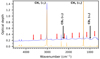 |
Fig. B.1. Spectra of IF3. Blue curve: raw infrared spectrum of IF3. The CH4 and CD4ν3 and ν4 absorption features are visible. Periodic oscillations induced by reflections on the ice interfaces are indicated with red arrows. Orange curve: infrared spectrum of IF3 corrected from the periodic oscillations. |
Appendix C: Optical images of the residues
Optical images of the ORs were acquired with the camera of the NanoSIMS. Images of OR1, OR2, OR4, OR5, OR6, OR7 and OR8 are displayed in Fig. C.1.
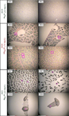 |
Fig. C.1. Optical images of the residues acquired with the camera of the NanoSIMS. White scale bars are 200 μm. Zones analyzed by NanoSIMS are indicated with blue boxes. |
Appendix D: Analytical conditions of the NanoSIMS acquisitions
The analytical conditions of the NanoSIMS sessions are reported in Table D.1. The ions collected during the acquisitions are: 12CH−, 12CD−, 12C14N−, 13C14N−, 12C15N−.
Summary of the analytical conditions of the NanoSIMS acquisitions performed on the ORs. The number of plans for CH− and CD− is indicated in parentheses.
Appendix E: Processing of the ice under ion-irradiation
IR spectra were acquired during the irradiation of the IFs to monitor their evolution. The formation of new species and the processing of the original ice constituents is evidenced by the attenuation of the features associated with pure ice components and the formation of new features as shown in Fig. E.1. The features identified in the IR spectra of the IFs before and during the irradiation and their attribution are reported in Table E.1
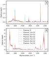 |
Fig. E.1. IR spectra acquired during the irradiation of IF7 (a) and IF8 (b), at different fluences. New species are formed during the irradiation, leading to new IR absorption features. |
List of IR features identified in the IFs prior and during the irradiation, adapted from Augé et al. (2019). The positions of features are indicated in parentheses when they differ from value reported in the literature.
Appendix F: Height measurements of the residues
Height measurements of the residues OR2, OR4, OR7 and OR8 were realized with an atomic force microscope. The residue OR2 has a bimodal height distribution resulting from the coexistence of patches and furrows where the amount matter is lower. The average height of the patches ranges from 130 to 160 nm whereas the average height of the furrows ranges between 30 and 60 nm. The measurements on OR4 were made on the a small patches region surrounding a circular empty area (visible in Fig. C.1, OR4). In that region, the average height of the organic matter patches is 106 nm, comparable to the value determined for OR2. Height measurements were acquired on two regions of interest on OR7. The first region is a large patch with high rims and smaller patches in the center. The height of the rim is ranging from about 600 to 900 nm while the heights of the smaller inner patches are ranging between 200 and 300 nm. The second region of interest is a large patch with a height varying between 250 and 750 nm. IR spectrum acquired on a solid droplet of OR8 displayed fringing pattern, such as those described in appendix B, caused by reflections at the interfaces. Assuming the refractive index n = 1.55 for the OR (Khare et al. 1994), Eq. B.1 gives a height of 5.7 μm. AFM measurements on two regions of interest on OR8 lead to heights ranging from 1 to 2.5 μm.
Appendix G: NanoSIMS images
NanoSIMS acquisitions were performed in different regions of interest on the ORs. 15N/14N, 13C/12C and D/H ratio images are shown in Fig. G.1 with a relative scale, as detailed in Sect. 3.3.
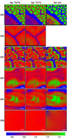 |
Fig. G.1. Ratio images derived from the NanoSIMS acquisitions. The color scale shows the relative variations of the isotopic composition from the mean value of the individual images. Left column: relative 15N/14N; center column: relative 13C/12C; relative D/H. No D/H image is shown for OR5 since no D-rich layered was added to the initial IF. The white scale bar is 5 μm. |
Appendix H: Comparison with the mixing model
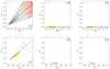 |
Fig. H.1. Comparison of the NanoSIMS data on OR5 (filled circles) and the IF5 mixing lines derived from the mixing model. Columns 1, 2 and 3 show the 15N/14N vs, 13C/12C, 15N/14N vs D/H and 13C/12C vs D/H compositions, respectively. Row a: mixing lines for αN = αC = αH = α. The value of α is indicated by the blue to red color contours. IF mixing lines with varying labeled layer compositions are displayed with dashed lines. The composition of the unlabeled ice is indicated in gray. Row b: the composition of IF5 is fixed and the mixing factors αN, αC, αH are set as free parameters. The value of the mixing factors are given by the gray scale on the top and right axes. The nominal mixing lines are plotted with bold dotted lines. |
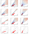 |
Fig. H.2. Comparison of the NanoSIMS data on OR7 (filled red circles) and the IF7 mixing lines derived from the mixing model. Columns 1, 2 and 3 show the 15N/14N vs, 13C/12C, 15N/14N vs D/H and 13C/12C vs D/H compositions, respectively. Row a, b and c: mixing lines for αN = αC = αH = α. Row a: the abundance of 15N2 is fixed and the abundances of CD4 and 13CO are varying. Row b: the abundance of CD4 is fixed and the abundances of 15N2 and 13CO are varying. Row c: the abundance of 13CO is fixed and the abundances of 15N2 and CD4 are varying. The value of α is indicated by the blue to red color contours. IF mixing lines with varying labeled layer compositions are displayed with dashed lines. The composition of the unlabeled ice is indicated in gray. Row d: the composition of IF7 is fixed and the mixing factors αN, αC, αH are set as free parameters. The value of the mixing factors are given by the gray scale on the top and right axes. The nominal mixing lines are plotted with bold dotted lines. |
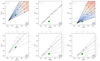 |
Fig. H.3. Comparison of the NanoSIMS data on OR8 (filled green circles) and the IF8 mixing lines derived from the mixing model. Columns 1, 2 and 3 show the 15N/14N vs, 13C/12C, 15N/14N vs D/H and 13C/12C vs D/H compositions, respectively. Row a: mixing lines for αN = αC = αH = α. The value of α is indicated by the blue to red color contours. IF mixing lines with varying labeled layer compositions are displayed with dashed lines. The composition of the unlabeled ice is indicated in gray. Row b: the composition of IF8 is fixed and the mixing factors αN, αC, αH are free parameters. The value of the mixing factors are given by the gray scale on the top and right axes. The nominal mixing lines are plotted with bold dotted lines. |
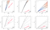 |
Fig. H.4. Comparison of the NanoSIMS data on OR6 (filled pink circles) and the IF6 mixing lines derived from the mixing model. Columns 1, 2 and 3 show the 15N/14N vs, 13C/12C, 15N/14N vs D/H and 13C/12C vs D/H compositions, respectively. Row a: mixing lines for αN = αC = αH = α. The value of α is indicated by the blue to red color contours. IF mixing lines with varying labeled layer compositions are displayed with dashed lines. The composition of the unlabeled ice is indicated in gray. Row b: the composition of IF6 is fixed and the mixing factors αN, αC, αH are set as free parameters. The value of the mixing factors are given by the gray scale on the top and right axes. The nominal mixing lines are plotted with bold dotted lines. |
Appendix I: Evolution of IF8 during annealing
Infrared spectra of IF8 were continuously acquired during the annealing of the ice film to monitor its evolution. Those spectra, for temperatures ranging from 15K to 100K are displayed in Fig. I.1. The decreasing intensity of the spectra with increasing temperature reflects the progressive sublimation of volatile species in IF8. Spectra of IF8 for temperature above 100K are not displayed as the IR signal lowers significantly. The evolution of NH3 bands at 3420-3130 cm−1 and 1070 cm−1 is consistent with the amorphous to metastable/crystalline phase transition of NH3 between 10K and 100K (Holt et al. 2004; Hudson et al. 2022). The significant decrease of features associated to CH4 at 3010 cm−1 and 1305 cm−1 between 30K and 40K reveals that most of the remaining CH4 in IF8 is sublimated in that temperature range.
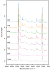 |
Fig. I.1. IR spectra acquired during the annealing of IF8 at different temperatures. |
Appendix J: Astrophysical context - Isotopically fractionated reservoirs on icy bodies
J.1. Isotopic fractionation of volatile reservoirs
The experiments presented in this paper show that organic matter formed from the irradiation of ices can preserve isotopic heterogeneities present in the ices, as sketched in the ideal layered configuration (Fig. 2). Ice mixtures in an astrophysical context are expected to be far more complex. Numerous studies evidenced the H, C and N isotopic fractionation of volatile species in the Solar System, as detailed by Ceccarelli et al. (2014), Bockelée-Morvan et al. (2015), Füri & Marty (2015) and Müller et al. (2022). In this section, we discuss possible isotopically fractionated volatile candidates of the Solar System.
H-bearing molecules in the coma of active comets are D-rich compared to VSMOW and the protosolar nebula value, δDPSN = −865‰ (Bockelée-Morvan et al. 2015, and references therein). DCN/HCN measured in comet C/1995 O1 Hale-Bopp is about 14 times higher than the D/H of terrestrial oceans, with δD ≈13, 700‰. A similar value, of δD = 14, 500 ± 1500‰, was derived for methane from in-situ mass spectrometry on comet 67/P Churyumov-Gerasimenko (hereafter, 67P) with the Rosetta/Rosina instrument (Müller et al. 2022). Methane was used in this study as the carrier of hydrogen and carbon atoms. Using the same instrument, Altwegg et al. (2019) derived a lower value of δD =(6100 ± 1300)‰ for NH3. Yet, for the protosolar nebula, chemical network models predict that D/H ratios may reach values up to 100 times larger in specific gaseous reservoirs within species such as CH3CHO, HCOOH, CH3CN, NH3 (Aikawa et al. 2012, 2018).
The primordial N2 reservoir was largely accreted by the Sun and the gas giants (Fletcher et al. 2014). Hence, its isotopic composition should be reflected by that of those objects. Marty et al. (2011) estimated the solar N isotopic composition to be δ15N =(−383 ± 8)‰, comparable to the isotopic composition of Jupiter measured in-situ by the Galileo spacecraft: δ15N =(−375 ± 80)‰ (Owen et al. 2001). If preserved in small bodies beyond the nitrogen snow line, primordial N2 ice should thus have a similar 15N-poor composition. Parallelly, NH3 and HCN in comets are found to be globally enriched in 15N compared to primordial N2. Based on CN and HCN emission lines, Bockelée-Morvan et al. (2008), Arpigny et al. (2003), Manfroid et al. (2009), estimated that the δ15N of HCN ranges between 240‰ and 960‰. Using optical observation of NH2, the principal photodissociation product of NH3, Shinnaka et al. (2016, 2014) and Rousselot et al. (2013) concluded that cometary NH3 has a comparable signature, with δ15N comprised between 430‰ and 2000‰, with no dependence on the type of comet. These compositions are reported in large period comets originating from the Oort cloud (’New’ and ’External’ in Shinnaka et al. (2016)), indicating that 15N-rich volatile species exist on icy bodies evolving at very large heliocentric distance (semimajor axis of about 10 000 au).
Similar spectroscopic measurements were used to derive the carbon isotope composition of volatile in comets. The δ13C in C2 and CN species ranges from ( − 58 ± 149)‰ to (118 ± 280)‰ (Wyckoff et al. 2000; Shinnaka et al. 2017; Manfroid et al. 2009; Rousselot et al. 2015). Estimations based on the HCN molecule in 3 comets led to substantially lower 13C/12C values: δ13C =(−194 ± 87)‰ (Jewitt et al. 1997), δ13C =(−215 ± 179)‰ (Bockelée-Morvan et al. 2008), δ13C =(−179 ± 105)‰ (Biver et al. 2016). More recently, Müller et al. (2022) estimated the isotopic compositions of the linear alkanes CH4, C2H6, C3H8, C4H10 in comet 67P to be ranging from δ13C = ( − 70 ± 134)‰ to (29 ± 107)‰, slightly lower but in agreement with measurements of CO and CO2 (Rubin et al. 2017; Hässig et al. 2017). Although these values suggest a heterogeneity of the 13C/12C ratio in comets, they do not drastically differ from the bulk Solar carbon isotope composition, estimated to be δ13C ≈ − 150 – −48‰ (Hashizume et al. 2004; Lyons et al. 2018). The large uncertainties associated with these measurements prevent to draw unambiguous conclusions on the C isotopic compositions of cometary volatiles.
J.2. Evolution of icy bodies
At the surface of an icy body, the transmission of isotopic heterogeneity from a parent ice to an OR requires the stable coexistence in the same location of condensed volatile species with distinct isotopic compositions.
Hypervolatile species, like N2, CH4 or CO, are detected at the surface of the large Trans-Neptunian Objects (TNOs) Pluto, Eris and Makemake (Grundy et al. 2016; Licandro et al. 2006; Lorenzi et al. 2015). Though, methane (Grundy et al. 2024) and carbon monoxide (De Prá et al. 2024) observed in the latter two may not have a primordial origin but rather formed by a subsequent thermal processing (Glein et al. 2024) and CO2 photodissociation. Smaller TNOs, orbiting at similar heliocentric distances, are unlikely to retain such molecules (Stern et al. 2019; Parhi & Prialnik 2023). Still, according to evolution models, comet-size bodies evolving at a larger heliocentric distance should preserve hypervolatile species at their surfaces. Parhi & Prialnik (2023) predict that a 9.5 km large body at 220 a.u. should retain most of its volatile content, including CO, after 4.6 Gyr, which is supported by the existence of CO- and N2-rich comets having an Oort Cloud origin (Biver et al. 2018; McKay et al. 2019; Anderson et al. 2023). Thus, the fractionated volatile species discussed in the Sect. J.1 (e.g N2, NH3, HCN, CH4, ...) possibly coexist at the surface of such objects.
Above ∼100 a.u., small bodies are not shielded by the heliosphere and the GCR dominate the energy deposition (Cooper et al. 2003). Unlike UV photons and low energy electrons, both contributing to the irradiation of the first hundred nanometers of the surface, GCR protons and heavy ions can penetrate much deeper, several centimeters to several meter deep, depending on their energy. Estimations of the dose deposited by GCR protons in the first 10-20 cm of an ice mantle in the Oort cloud, during 4.6 Gyr, range from about 40 eV⋅molec−1 (Donn 1976; Moore et al. 1983; Gerakines et al. 2000) to 600 eV⋅molec−1 (Strazzulla & Johnson 1991; Moore et al. 2001). The doses deposited in the experiments presented here (8.2 – 21.8 eV⋅molec−1) correspond to an irradiation lasting between 60 Myr and 2.5 Gyr, consistent with the lifetime of volatile ice mantles at the surface of Oort cloud objects. Importantly, because the radiolysis process is proportional to the square of the ion’s atomic number, Z2, (Dartois et al. 2023), the contribution of swift heavy ions (Z> 2) to the energy deposition cannot be neglected and possibly account for as much as the protons’ contribution. As the timescales of irradiation discussed above are derived from the energy deposition of protons only, they should thus be considered as upper limits. These timescales can also be drastically lowered when considering smaller depth since the energy deposition highly depends on the penetration depth of the ions (Cooper et al. 2003). Consequently, the processing of icy bodies surfaces leading to the production of OR may only require a few tens Myr, and may have happened early in the Solar System history.
The annealing process that leads to the degassing of hypervolatile ices, the concentration of radiolytic precursors and the formation of the refractory OR can either take place during the journey of the parent body along an eccentric orbit or when the parent body enters the inner Solar System after being ejected from its initial orbit (e.g., in the Oort Cloud). In the former case, episodes of irradiation and sublimation can happen sequentially, resulting in the production of a stacked organic crust, in a similar fashion to what is expected for TNOs (Stern et al. 2019; Grundy et al. 2020). In the latter case, the formation of the refractory residue may be effective late in the evolution of the parent body.
All Tables
Summary of the analytical conditions of the NanoSIMS acquisitions performed on the ORs. The number of plans for CH− and CD− is indicated in parentheses.
List of IR features identified in the IFs prior and during the irradiation, adapted from Augé et al. (2019). The positions of features are indicated in parentheses when they differ from value reported in the literature.
All Figures
|
Fig. 1. Technical scheme of the IGLIAS chamber adapted from Augé et al. (2019). Experimental windows are disposed on a rotary head at the center of the chamber and in contact with a helium cryostat cooling system and a heating system. Ice samples are formed by the condensation of gas injected on the cooled windows. The chamber is connected to the IRRSUD ion beam at GANIL. The evolution of the IF during irradiation is monitored by a Fourier transform infrared spectrometer (FTIR) with a 12° incidence angle. A quadrupolar mass spectrometer (QMS) is connected to the chamber to monitor the gas phase. |
| In the text | |
|
Fig. 2. Schematic view of the experimental protocol. The IFs are condensed by injection of a gas mixture on a substrate window at 10 K. A first isotopically unlabeled ice layer is deposited (light blue, (1)), followed by a thin layer of isotopically labled ice (red, (2)) and a final unlabeled ice layer (light blue, (3)). The whole IF is irradiated by heavy ions (4), resulting in the radiolysis of initial species and the formation of new molecules (5). At the end of the irradiation, the IF is slowly annealed from 10 K to 300 K, causing the sublimation of remaining volatile species (6) and the formation of a refractory OR (7). |
| In the text | |
|
Fig. 3. Stopping power of ions in the ice films. Left axis and solid lines: Evolution of the electronic stopping power of ions used in the experimental sessions as a function of their penetration depth in a 14N2-12CH4 (9:1) IF, modeled with the SRIM code. Right axis and dashed lines: evolution of the nuclear over electronic stopping powers ratio as function of the penetration depths in the IFs. Filled circles indicate the size of the IFs irradiated during the experiments. |
| In the text | |
|
Fig. 4. Mosaic of optical images of the residues OR7 (a.) and OR8 (c.), formed on Silicon windows during the 2021 session. Images (b.) and (d.) are close-up images. Residue OR7 and OR8 were formed during the same session from N2-CH4 and a NH3-CH4 ice mixtures, respectively. The different structures of the residues are most probably due to the different chemical composition of the starting ice (see text). |
| In the text | |
|
Fig. 5. IR spectra of OR3, OR5, OR7, and OR8. The spectrum of the OR reported by Augé et al. (2019) is reported with a dashed black line. |
| In the text | |
|
Fig. 6. Graphs of the distribution of isotopic values measured in the residues OR4 (blue), OR5 (orange), OR6 (pink), OR7 (red), and OR8 (green). (a): 15N/14N against 13C/12C. (b): 15N/14N against D/H. Residues OR4, OR5, and OR6 were formed during the 2020 session and residues OR7 and OR8 during the 2021 session. Residues formed during the same session experienced the same conditions, that is, they formed on the same substrate, irradiated with the same ions, and experienced the same annealing. |
| In the text | |
|
Fig. 7. Ratio images derived from the NanoSIMS acquisitions. The color scale shows the relative variations of the isotopic composition from the mean value of the individual images. Left column: Relative 15N/14N. Center column: Relative 13C/12C; relative D/H. Images of residues OR4, OR5, OR6, OR7, and OR8 are shown in rows one, two, three, four, and five, respectively. No D/H image is shown for OR5 since no D-rich layer was added to the initial IF. The white scale bar is 5 μm. |
| In the text | |
|
Fig. 8. Comparison of the NanoSIMS data on OR4 (filled circles) and the IF4 mixing lines derived from the mixing model. Columns 1, 2, and 3 show the 15N/14N versus 13C/12C, 15N/14N versus D/H, and 13C/12C versus D/H compositions, respectively. Row a: mixing lines for αN = αC = αH = α. The value of α is indicated by the blue to red color contours. IF mixing lines with varying labeled layer compositions are displayed with dashed lines. The composition of the unlabeled ice is indicated in gray. Row b: the composition of IF4 is fixed and the mixing factors αN, αC, αH are free parameters. The value of the mixing factors are given by the gray scale on the top and right axes. The nominal mixing lines are plotted with bold dotted lines. |
| In the text | |
|
Fig. B.1. Spectra of IF3. Blue curve: raw infrared spectrum of IF3. The CH4 and CD4ν3 and ν4 absorption features are visible. Periodic oscillations induced by reflections on the ice interfaces are indicated with red arrows. Orange curve: infrared spectrum of IF3 corrected from the periodic oscillations. |
| In the text | |
|
Fig. C.1. Optical images of the residues acquired with the camera of the NanoSIMS. White scale bars are 200 μm. Zones analyzed by NanoSIMS are indicated with blue boxes. |
| In the text | |
|
Fig. E.1. IR spectra acquired during the irradiation of IF7 (a) and IF8 (b), at different fluences. New species are formed during the irradiation, leading to new IR absorption features. |
| In the text | |
|
Fig. G.1. Ratio images derived from the NanoSIMS acquisitions. The color scale shows the relative variations of the isotopic composition from the mean value of the individual images. Left column: relative 15N/14N; center column: relative 13C/12C; relative D/H. No D/H image is shown for OR5 since no D-rich layered was added to the initial IF. The white scale bar is 5 μm. |
| In the text | |
|
Fig. H.1. Comparison of the NanoSIMS data on OR5 (filled circles) and the IF5 mixing lines derived from the mixing model. Columns 1, 2 and 3 show the 15N/14N vs, 13C/12C, 15N/14N vs D/H and 13C/12C vs D/H compositions, respectively. Row a: mixing lines for αN = αC = αH = α. The value of α is indicated by the blue to red color contours. IF mixing lines with varying labeled layer compositions are displayed with dashed lines. The composition of the unlabeled ice is indicated in gray. Row b: the composition of IF5 is fixed and the mixing factors αN, αC, αH are set as free parameters. The value of the mixing factors are given by the gray scale on the top and right axes. The nominal mixing lines are plotted with bold dotted lines. |
| In the text | |
|
Fig. H.2. Comparison of the NanoSIMS data on OR7 (filled red circles) and the IF7 mixing lines derived from the mixing model. Columns 1, 2 and 3 show the 15N/14N vs, 13C/12C, 15N/14N vs D/H and 13C/12C vs D/H compositions, respectively. Row a, b and c: mixing lines for αN = αC = αH = α. Row a: the abundance of 15N2 is fixed and the abundances of CD4 and 13CO are varying. Row b: the abundance of CD4 is fixed and the abundances of 15N2 and 13CO are varying. Row c: the abundance of 13CO is fixed and the abundances of 15N2 and CD4 are varying. The value of α is indicated by the blue to red color contours. IF mixing lines with varying labeled layer compositions are displayed with dashed lines. The composition of the unlabeled ice is indicated in gray. Row d: the composition of IF7 is fixed and the mixing factors αN, αC, αH are set as free parameters. The value of the mixing factors are given by the gray scale on the top and right axes. The nominal mixing lines are plotted with bold dotted lines. |
| In the text | |
|
Fig. H.3. Comparison of the NanoSIMS data on OR8 (filled green circles) and the IF8 mixing lines derived from the mixing model. Columns 1, 2 and 3 show the 15N/14N vs, 13C/12C, 15N/14N vs D/H and 13C/12C vs D/H compositions, respectively. Row a: mixing lines for αN = αC = αH = α. The value of α is indicated by the blue to red color contours. IF mixing lines with varying labeled layer compositions are displayed with dashed lines. The composition of the unlabeled ice is indicated in gray. Row b: the composition of IF8 is fixed and the mixing factors αN, αC, αH are free parameters. The value of the mixing factors are given by the gray scale on the top and right axes. The nominal mixing lines are plotted with bold dotted lines. |
| In the text | |
|
Fig. H.4. Comparison of the NanoSIMS data on OR6 (filled pink circles) and the IF6 mixing lines derived from the mixing model. Columns 1, 2 and 3 show the 15N/14N vs, 13C/12C, 15N/14N vs D/H and 13C/12C vs D/H compositions, respectively. Row a: mixing lines for αN = αC = αH = α. The value of α is indicated by the blue to red color contours. IF mixing lines with varying labeled layer compositions are displayed with dashed lines. The composition of the unlabeled ice is indicated in gray. Row b: the composition of IF6 is fixed and the mixing factors αN, αC, αH are set as free parameters. The value of the mixing factors are given by the gray scale on the top and right axes. The nominal mixing lines are plotted with bold dotted lines. |
| In the text | |
|
Fig. I.1. IR spectra acquired during the annealing of IF8 at different temperatures. |
| In the text | |
Current usage metrics show cumulative count of Article Views (full-text article views including HTML views, PDF and ePub downloads, according to the available data) and Abstracts Views on Vision4Press platform.
Data correspond to usage on the plateform after 2015. The current usage metrics is available 48-96 hours after online publication and is updated daily on week days.
Initial download of the metrics may take a while.