| Issue |
A&A
Volume 694, February 2025
|
|
|---|---|---|
| Article Number | A218 | |
| Number of page(s) | 15 | |
| Section | Extragalactic astronomy | |
| DOI | https://doi.org/10.1051/0004-6361/202451448 | |
| Published online | 18 February 2025 | |
Revealing the hidden cosmic feast: A z = 4.3 galaxy group hosting two optically dark, efficiently star-forming galaxies
1
Cosmic Dawn Center (DAWN), Copenhagen, Denmark
2
DTU Space, Technical University of Denmark, Elektrovej 327, 2800 Kgs. Lyngby, Denmark
3
Instituto de Física y Astronomía, Universidad de Valparaíso, Avda. Gran Bretana 1111, Valparaíso, Chile
4
Instituto de Física, Pontificia Universidad Católica de Valparaíso, Casilla 4059, Valparaíso, Chile
5
Institute of Astronomy and Astrophysics, Academia Sinica, 11F of Astronomy-Mathematics Building, No.1, Sec. 4, Roosevelt Rd, Taipei 106216, Taiwan, ROC
6
Hiroshima Astrophysical Science Center, Hiroshima University, 1-3-1 Kagamiyama, Higashi-Hiroshima, Hiroshima 739-8526, Japan
7
National Astronomical Observatory of Japan, 2-21-1, Osawa, Mitaka, Tokyo, Japan
8
AIM, CEA, CNRS, Université Paris-Saclay, Université Paris Diderot, Sorbonne Paris Cité, 91191 Gif-sur-Yvette, France
9
Leiden Observatory, Leiden University, NL-2300 RA Leiden, The Netherlands
10
Purple Mountain Observatory, Chinese Academy of Sciences, 10 Yuanhua Road, Nanjing 210023, China
11
European Southern Observatory, Karl-Schwarzschild-Str. 2, 85748 Garching, Germany
⋆ Corresponding authors; malte.brinch@uv.cl; shuji@dtu.dk
Received:
10
July
2024
Accepted:
9
January
2025
We present the confirmation of a compact galaxy group candidate, CGG-z4, at z = 4.3 in the COSMOS field. This structure was identified by two spectroscopically confirmed z = 4.3 Ks-dropout galaxies with ALMA 870 μm and 3 mm continuum detections, surrounded by an overdensity of near infrared-detected galaxies with consistent photometric redshifts of 4.0 < z < 4.6. The two ALMA sources, CGG-z4.a and CGG-z4.b, have been detected with both CO(4–3) and CO(5–4) lines, whereby [CI](1–0) has been detected on CGG-z4.a, and H2O(11, 0–10, 1) absorption detected on CGG-z4.b. We modeled an integrated spectral energy distribution (SED) by combining the far-infrared-to-radio photometry of this group and estimated a total star formation rate of ∼2000 M⊙ yr−1, making it one of the most star-forming groups known at z > 4. Their high CO(5–4)/CO(4–3) ratios indicate that each respective interstellar medium (ISM) is close to thermalization, suggesting either high gas temperatures, high densities, and/or high pressure; whereas the low [CI](1–0)/CO(4–3) line ratios indicate high star formation efficiencies. With the [CI]-derived gas masses, we found the two galaxies have extremely short gas depletion times of 99 Myr and < 63 Myr, respectively, suggesting the onset of quenching. With an estimated halo mass of log(Mhalo [M⊙]) ∼ 12.8, we find that this structure is likely to be in the process of forming a massive galaxy cluster.
Key words: galaxies: evolution / galaxies: formation / galaxies: high-redshift / galaxies: ISM / galaxies: groups: individual: CCG-z4
© The Authors 2025
 Open Access article, published by EDP Sciences, under the terms of the Creative Commons Attribution License (https://creativecommons.org/licenses/by/4.0), which permits unrestricted use, distribution, and reproduction in any medium, provided the original work is properly cited.
This article is published in open access under the Subscribe to Open model. Subscribe to A&A to support open access publication.
1. Introduction
Within the modern ΛCDM paradigm, a major goal is to understand the formation and evolution of massive galaxies (M⋆ > 1011 M⊙) and the structures they inhabit (clusters and groups). For a ΛCDM cosmology, massive galaxies are thought to form through the hierarchical clustering of lower mass galaxies and their dark matter halos (Springel et al. 2005). From cosmological simulations, the growth of massive galaxies has been shown to be in a heightened phase prior to cosmic noon (z > 2) due to a combination of in situ gas accretion and the merging of low-mass (M⋆ ≲ 1010 M⊙) satellite galaxies (Hopkins et al. 2009; Oser et al. 2010; Benson et al. 2012; Hirschmann et al. 2012). Overdense structures such as protoclusters or galaxy groups are prime locations to investigate the growth of massive galaxies, as these structures initially formed in the peaks of the primordial density field. They are thought to undergo a downsizing effect, where the galaxies in the overdense structure (especially in the center of the structure) will become more evolved, compared to the field population (Overzier 2016; Chiang et al. 2017; Marrone et al. 2018). These overdense structures are typically found through either the use of large-scale surveys of specific types of galaxies such as Lyman-break galaxies or Lyman-alpha emitters (see Harikane et al. 2019; Brinch et al. 2023, 2024). They can also be found using signpost galaxies such as submillimeter (submm) galaxies (SMGs) or quasi-stellar objects (QSOs) that are biased tracers of overdensities, where their nearby environment can then be investigated (see Capak et al. 2011; Walter et al. 2012; Lewis et al. 2018; Calvi et al. 2023). Wide-field submillimeter-millimeter (submm/mm) and interferometric observations with instruments such as Submillimetre Common-User Bolometer Array 2 (SCUBA-2) on the James Clark Maxwell Telescope (JCMT), Northern Extended Millimeter Array (NOEMA), and the Atacama Large Millimeter/submillimeter Array (ALMA) have allowed for the study of massive, highly star-forming galaxies in the high-redshift Universe thanks to their high spectral coverage and sensitivity (Dannerbauer et al. 2014; Oteo et al. 2018; Miller et al. 2018). In conjunction with optical and near-infrared (NIR) surveys, these observations enable us to identify and study the dense and compact structures where these galaxies assemble (e.g., Wang et al. 2016; Daddi et al. 2021, 2022; Jones et al. 2017; Díaz-Santos et al. 2018; Cooper et al. 2022; Ginolfi et al. 2022; Sillassen et al. 2022, 2024; Jin et al. 2023, 2024a).
Meanwhile, studies have revealed a population of optically/NIR dark dusty star-forming galaxies (DSFGs) that drop out in deep optical images (Smail et al. 1999, 2021; Higdon et al. 2008; Wang et al. 2019; Algera et al. 2020; Talia et al. 2021; Gómez-Guijarro et al. 2022; Shu et al. 2022; van der Vlugt et al. 2023; Xiao et al. 2023). They are found to play a critical role in the dust-obscured cosmic star-formation density (SFRD), with a contribution of up to 50% at high redshift and likely dominate at the massive end (log(M⊙/M⊙) > 10.5) of the stellar mass function (SMF) at z ∼ 3 − 7 (Wang et al. 2019). With the advent of the James Webb Space Telescope (JWST), The search for optically faint and dark galaxies has been pushed to redshifts of z ∼ 8, where they have been shown to be an important contribution to the high-mass end of the galaxy stellar mass function and the cosmic SFRD up to z ∼ 7 − 8. Furthermore, a significant fraction of z > 3 galaxies, especially massive galaxies, has gone unaccounted for (Barrufet et al. 2023; Gottumukkala et al. 2024). However, the majority of literature studies of this population at high redshift rely heavily on photometric redshifts. The spectroscopically confirmed sample of optically dark galaxies is still small, with their environments and ISM properties remaining largely unknown.
In this work, we present the discovery of a compact galaxy group (which we dub CGG-z4) and study the member galaxies’ star formation and ISM properties. This paper is organized as follows. We describe the observational data and selection in Sect. 2. Section 3 describes the methods for redshift confirmation, spectral stacking, and SED fittings. In Sect. 4, we present the results and analysis, including different physical properties such as SFR and gas mass estimates. We discuss relevant science in Sect. 5 and summarize our conclusions in Sect. 6. Throughout the paper, we have adopted a standard ΛCDM cosmology with H0 = 70 km s−1 Mpc−1, Ωm = 0.3, and ΩΛ = 0.7. All magnitudes are expressed in the AB system (Oke 1974). We adopted a Chabrier (2003) stellar initial mass function (IMF). The results are reported with uncertainties within the 68% confidence interval.
2. Selection and data
2.1. Selection
CGG-z4.a was initially selected as a radio source by the VLA 3GHz Large Program in the COSMOS field (Smolčić et al. 2017) at 8σ. It was included in the COSMOS Super-deblended catalog (Jin et al. 2018) as an additional radio prior in combination with the low-angular resolution Herschel bands and with no optical/NIR counterpart in the COSMOS2015 catalog (Laigle et al. 2016). It was observed by an ALMA 3 mm line scan as a bright SCUBA-2 source in the Simpson et al. (2019) map, a part of the ALMA project 2021.1.00246.S, (PI: C. Chen). Our initial FIR SED analysis with deblended FIR photometry suggested a zFIR ∼ 6; this was followed up with an ALMA 3 mm line scan in program 2022.1.00884.S (PI: R. Gobat). CGG-z4.b has been observed in the ALMA pointing as well, and is also included among the radio sources in the Smolčić et al. (2017) catalog at 8σ. The remaining candidate members of CGG-z4 are selected from the COSMOS2020 CLASSIC catalog (Weaver et al. 2022). We adopted a photometric redshift selection of 4.0 < zphot < 4.6 from the EAZY spectral energy distribution (SED) fitting (Brammer et al. 2008) with UV/optical to NIR photometry in COSMOS2020, corrected for Galactic extinction using the Schlafly & Finkbeiner (2011) dust map. The galaxies are not part of the area covered by the JWST treasury program COSMOS-Web (ID:1727, PI: J. Kartaltepe, Casey et al. 2023).
2.2. ALMA
The two ALMA 3 mm line scan programs continuously cover the frequency range from 84.1 to 113.2 GHz in Band 3 (Claude et al. 2006). Program 2021.1.00246.S yielded a continuum sensitivity of 0.02 mJy/Beam, an angular resolution of 1.6″ and a velocity resolution of 84 km/s observed over a 26 min scan. Program 2022.1.00884.S yielded a continuum sensitivity of 0.02 mJy/Beam, an angular resolution of 1.1″ and a velocity resolution of 23 km/s observed over three 20 min scans. ALMA 870 μm continuum detections were obtained as part of the program 2016.1.00463.S (PI: Y. Matsuda), in which CGG-z4 was observed over 0.7 min in Band 7 (Mahieu et al. 2005; Maier et al. 2005) with a continuum sensitivity of 0.27 mJy/Beam, an angular resolution of 0.8″ and a velocity resolution of 27 km/s. The ALMA data were reduced and calibrated using the standard ALMA CASA pipeline (McMullin et al. 2007). Following our established pipeline from Jin et al. (2019, 2022, 2024b), the calibrated measurement sets were then converted to uvfits format for further analysis in uv space with the GILDAS software (Gildas Team 2013). For the galaxies with a continuum detection, the spectrum was extracted using Gildas uv_fit, in which we fit uv visibility at each frequency using a point source model fixed at the position of continuum peak. For sources without strong continuum detection, their spectra were extracted based on positions from the COSMOS2020 catalog. We note that program 2021.1.00246.S contains 20 spectral windows (SPWs), and project 2021.1.00246.S contains 12 SPWs. We extracted the 3 mm 1D spectrum of each SPW and combined the spectra of all SPWs in the observed frame to enhance the signal-to-noise ratio (S/N) at overlapped frequencies. This resulted an average 1σ spectral line sensitivity of 0.05 Jy km s−1 beam−1 over a 500 km s−1 width in Band 3. The continuum fluxes were measured by combining all line-free channels and fitting the sources in uv space with point-source models. The clean residuals indicate the sources are well-fitted and are unresolved in the dust continuum. The resulting synthesized beam size is ≈2.7″ for the 3 mm data, while the 870 μm data has a synthesized beam of ≈0.8″. The spectra of CGG-z4.a and CGG-z4.b are shown in Fig. 1, while line and continuum maps are shown in Fig. 2.
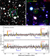 |
Fig. 1. Images and spectra highlighting the member galaxies of the CGG-z4 galaxy group. Top left: VISTA Ks images overlaid with cyan SCUBA-2 850 μm contours in steps of 3, 5 and 7σ. Photometric redshift candidate members in the range 4.0 < z < 4.6 are highlighted with red dashed circles. Galaxies with ALMA continuum detections are highlighted as magenta-dashed circles. The green square highlights the region of the right image. Top right: VISTA RGB color images of CGG-z4 at z ∼ 4.3 using the Ks (red), J (green), and i (blue) bands. Two spectroscopically confirmed galaxies have ALMA 3 mm and 870 μm continuum emission shown as green and yellow contours. Contours are shown at levels 5, 7, and 10σ. ALMA beam sizes and an image scale are shown in the lower right corner. The RGB frames are composed using linear scales with identical limits. Bottom: ALMA 3 mm spectra for galaxies with emission line detections. The detected lines are highlighted in yellow with their names labeled. The red line shows Gaussian fits to the CO emission lines and a power law fit to the continuum that increases with frequency following the expression ν3.7. |
2.3. Ancillary data
We use VISTA images from Weaver et al. (2022) for visualization, as shown in Fig. 1. To identify the candidate members in this group, we utilized the optical/NIR photometry and photometric redshifts in the COSMOS2020 catalog (Weaver et al. 2022). We note that the area of CGG-z4 was masked in the COSMOS2020 Farmer catalog, so instead we used the COSMOS2020 Classic catalog which fully cataloged galaxies in this area. To constrain the FIR SED of CGG-z4, we make use of MIPS (Le Floc’h et al. 2009), Herschel (Lutz et al. 2011; Oliver et al. 2012), SCUBA-2 (Simpson et al. 2019), and VLA images (Smolčić et al. 2017) to measure the FIR-to-radio photometry with the Super-deblending technique (Jin et al. 2018; Liu et al. 2018).
3. Method
3.1. Line detections and Redshift determination
We use the LMfit package (Newville et al. 2014) to fit the emission lines and continuum simultaneously. Emission lines were fitted as Gaussians. When multiple emission lines were present in the same spectra, we fixed the sigma value of the Gaussian to be the same when performing the fitting, which, in turn, means the full width at half maximum (FWHM) is fixed. the continuum is fitted as a power law using the formula y = A × νP, where A is the amplitude and P = 3.7 following Magdis et al. (2012), Jin et al. (2022). The line fits are shown in Fig. 1 and the derived properties are reported in Table 1. With line detections of CO(4–3) and CO(5–4), we measured a redshift of z = 4.331 ± 0.001 and 4.324 ± 0.001 for CGG-z4.a and b, respectively. The CO(4–3) lines are detected with an integrated line flux significance of 11.6σ, 8.4σ, and CO(5–4) is detected with 7.7σ, 4.8σ respectively. The redshift difference between the two sources is Δz = 0.007, which is equivalent to an on-sky projected line of sight distance of 0.829 pMpc (395 km/s). Notably, we also detect the [CI](1–0) emission line in CGG-z4.a with 4.3σ and ortho-H2O(11, 0–10, 1) absorption line in CGG-z4.b with 3.5σ. The detection of water absorption in CGG-z4.b adds to a growing list of lines observed in the high redshift universe, including the H2O(11, 0–10, 1) absorption in HFLS3 at z = 6.34 (Riechers et al. 2022) and in ID 9316 at z = 4.07 (Jin et al. 2022). The water line is an indicator that the galaxy is currently undergoing a starburst, as the intense radiation field from the starburst results in a line excitation temperature that is lower than the CMB temperature, resulting in absorption against the CMB. This also allows the line to be a probe of the CMB temperature (Riechers et al. 2022).
Line fitting results for CGG-z4 group galaxies.
3.2. Spectral stacking
To identify potential CO emissions from the optical/NIR-detected members, we extracted spectra at the positions of all candidate galaxy group members and stacked them at the redshift of CGG-z4.a. We calculated the S/Ns at CO(5–4) and CO(4–3) frequencies and we found no definitive detections at the 2σ level (0.06 Jy km/s for CO(5–4) and 0.04 Jy km/s for CO(4–3)), nor a continuum detection. This indicates that the two optically dark galaxies dominate the total SFR and gas content of this group.
3.3. SED fitting
To estimate the physical characteristics of the CGG-z4.a and CGG-z4.b, we performed a detailed SED analysis by fitting the integrated FIR, (sub-)mm, and radio photometry. The integrated FIR to radio photometry is measured using the Super-deblending technique (Jin et al. 2018; Liu et al. 2018), following the identical pipeline adopted for high-redshift groups as in Daddi et al. (2021), Sillassen et al. (2022, 2024), Zhou et al. (2024). We used the SED fitting code MICHI2 (Liu 2020; Liu et al. 2021) that simultaneously fits components of stellar (Bruzual & Charlot 2003), mid-IR active galactic nuclei (AGNs, Mullaney et al. 2011) and dust (Draine & Li 2007), as well as a radio component derived from IR-radio correlation (Magnelli et al. 2015), without the assumption of energy balance. Given the optically dark nature of CGG-z4.a and CGG-z4.a, we fit the MIPS/24 μm, Herschel, SCUBA2, and ALMA photometry, with a mid-IR AGN, warm photodissociation region (PDR), and cold and ambient dust components. Figure 3 shows the full fit, with the photometry used shown in Table A.1. For comparison with the ALMA and radio data where the two galaxies are resolved, we scaled the combined SED with the ALMA 870 μm flux of CGG-z4.a and CGG-z4.b. We observe that scaled SED fits align with the data, with the exception of the radio data of CGG-z4.a, which is below the expected value from the IR-radio correlation.
When fitting the optically detected COSMOS2020 galaxies, it should be noted that the SED fits from EAZY are a linear combination of 12 preselected flexible stellar population synthesis (FSPS) templates. EAZY primarily excels in determining the redshift probability distribution of large galaxy samples. Other SED fitting codes are more suited when estimating the physical properties of individual galaxies. To that end, we use the SED fitting code BAGPIPES (Carnall et al. 2018) to fit the COSMOS2020 classic photometry for physical parameters like stellar mass and star formation rate (SFR). We followed the approach of Carnall et al. (2023), Heintz et al. (2023), Jin et al. (2023) and assumed a constant star formation history (SFH) and the attenuation curve of Salim et al. (2018), which mimics a bursty SFH on short timescales. A Salim et al. (2018) curve better represents low-mass, low-metallicity galaxies. We note that we tried using an exponential SFH, which resulted in virtually identical results since our current data only allows us to probe the recent burst for the optical/NIR galaxies due to the outshining effect from the massive young stars in the galaxies. We ran BAGPIPES with the following parameters: formation mass log(M⋆) ∈ [6.0:12.0] log(M⊙), metallicity Z∈[0.01:2.00] Z⊙, reddening Av ∈ [0.0:4.0], and the U parameter, which is the strength of the nebular radiation field to log(U)∈[−4.0 : −1.0]. We ran the fitting for each COSMOS2020 galaxy at the spectroscopic redshift of CGG-z4.a (z = 4.331), assuming they are all part of the galaxy group. The resulting SED fits are shown in Fig. B.1 and a summary of all the values obtained from the SED fitting is shown in Table C.1. We note that allowing the photometric redshift to vary in BAGPIPES results in changes to the posterior fit values that are (at most) at the 1σ level, with the exception being the age of ID361346 having a higher metallicity of  and a younger age of
  . This does not change any of the conclusions drawn in this paper.
4. Results and analysis
4.1. A z ≈ 4.3 compact galaxy group
Figure 1 presents color images of CGG-z4, comprised of Hyper Suprime-Cam (HSC) and Visible and Infrared Survey Telescope for Astronomy (VISTA) bands with SCUBA2 and ALMA contours overlaid. The Ks-band image highlights the region where the original SCUBA source was detected, while the Ks,J,i true color image shows the ALMA continuum contours of the two optical/NIR dark sources, as well as the optically/NIR, detected galaxies that are within the COMOS2020 catalog. The ALMA 3 mm spectra for the two sources with multiple line detections, CGG-z4.a and CGG-z4.b, are shown in the bottom panel of Fig. 1. CGG-z4.b is within 1″ of a z = 0.8 galaxy identified in the COSMOS2020 catalog with ID 357498. Similar to the SMGs of Smail et al. (2021), CGG-z4.a and CGG-z4.b are not detected in the Ks-band with Ks > 25.3 mag in the COSMOS2020 catalog (Weaver et al. 2022), with the combination of no detection blueward of the Ks-band classifying them as Ks-band dropouts. Figure 2 Shows the ALMA 3 mm continuum map and line emission maps for CGG-z4.a and CGG-z4.b, with the members found in COSMOS2020 overlaid. We see a high sky overdensity of galaxies within a small region, with 13 galaxies over a region of 13″ × 31″ (89 × 209 kpc2). For any galaxy group or protocluster to grow into a cluster over time, it requires material (other halos with galaxies and gas) to be fed into the structure. It is therefore important to consider the large-scale environment that the group is part of when considering if it will end up as a cluster by z = 0. Performing an overdensity analysis for galaxies at z = 4.0 − 4.6 in the COSMOS field in the same manner as Brinch et al. (2023), utilizing a weighted adaptive kernel estimator and including the spectroscopic redshifts of Khostovan et al. (in prep.), we find that CGG-z4 appears to be in an overdense environment at the 3σ level (δOD = 2.16). This significance is similar to other studies that have used SMGs as tracers of overdense environments (see Calvi et al. 2023, and references therein).
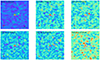 |
Fig. 2. ALMA line and continuum maps, with black lines showing the positive contours and white dashed lines the negative contours, both starting from 2σ to 6σ in steps of 2σ; except for the continuum map, where the contours start from 3σ to 12σ with 3σ steps. The size and orientation of the beam are indicated in the lower left corner in red. Magenta crosses mark COSMOS2020 sources. |
4.2. Stellar mass
The results of EAZY and BAGPIPES SED fitting are listed in Table C.1. The EAZY median redshift in the tables is shown to highlight the uncertainty of the redshifts. Given the optically dark nature of CGG-z4.a and b, coupled with the fact that they are only detected in IRAC channel 2, we applied two methods to estimate their stellar masses. First, we scaled their IRAC channel 2 peak fluxes to the IRAC fluxes of the COSMOS2020 sources with photometric redshifts between 4.0 < z < 4.6 and then scaled the average stellar mass to CGG-z4.a and b. This yielded log M*/M⊙ ∼ 10.4 for both galaxies. A caveat is that the inferred stellar masses are prone to be uncertain as they are based on one-band photometry. Second, given their robust detections in sub-mm and mm wavelengths, we inferred their stellar masses using dust mass with empirical stellar-to-dust mass ratios. By fitting optically thick blackbody models to their FIR and ALMA photometry (e.g., Lamperti et al. (2019)), we obtained dust masses of ![$ \rm log(M_{\mathrm{dust}}\,\rm [M_{\odot}]) = 9.10^{+0.29}_{-0.28} $](/articles/aa/full_html/2025/02/aa51448-24/aa51448-24-eq3.gif) and
and ![$ \rm log(M_{\mathrm{dust}}\,\rm [M_{\odot}]) = 8.80^{+0.29}_{-0.29} $](/articles/aa/full_html/2025/02/aa51448-24/aa51448-24-eq4.gif) for a and b, respectively. Then we adopted a range of stellar-to-dust mass ratios M*/Mdust = 50 − 100, a typical value for starburst galaxies at high-redshifts (Donevski et al. 2020). We obtained stellar masses of
for a and b, respectively. Then we adopted a range of stellar-to-dust mass ratios M*/Mdust = 50 − 100, a typical value for starburst galaxies at high-redshifts (Donevski et al. 2020). We obtained stellar masses of ![$ \rm log(M_{\mathrm{\star}}\,\rm [M_{\odot}]) = 10.98^{+0.30}_{-0.37} $](/articles/aa/full_html/2025/02/aa51448-24/aa51448-24-eq5.gif) and
and ![$ \rm log(M_{\mathrm{\star}}\,\rm [M_{\odot}]) = 10.68^{+0.30}_{-0.38} $](/articles/aa/full_html/2025/02/aa51448-24/aa51448-24-eq6.gif) . The Mdust-based stellar masses are 0.62 and 0.29 dex higher than IRAC-scaled ones, which is understandable as the IRAC fluxes (rest-frame of 0.8 μm) can be severely attenuated in optically dark galaxies (e.g., Kokorev et al. 2023). To reconcile the results from the two methods, we conservatively adopted the average stellar masses with uncertainties compassing both results, as listed in Table C.1. Future observations with JWST will be essential to constrain their stellar content robustly.
. The Mdust-based stellar masses are 0.62 and 0.29 dex higher than IRAC-scaled ones, which is understandable as the IRAC fluxes (rest-frame of 0.8 μm) can be severely attenuated in optically dark galaxies (e.g., Kokorev et al. 2023). To reconcile the results from the two methods, we conservatively adopted the average stellar masses with uncertainties compassing both results, as listed in Table C.1. Future observations with JWST will be essential to constrain their stellar content robustly.
4.3. Halo mass
We applied five methods to estimate the dark matter halo mass. We followed the identical pipeline by Sillassen et al. (2024), which was intricately designed for eight massive groups at 1.5 < z < 4 in the COSMOS field, where they applied six methods for estimating the dark matter masses, including the stellar-mass-to-halo-mass relations (SHMR), overdensity with galaxy bias, and NFW profile fitting to radial stellar mass densities (see details in Sillassen et al. 2024, Sect. 4.4).
First, using the stellar mass of the central galaxy CGG-z4.a with a SHMR from Behroozi et al. (2013), we obtained a lower limit of halo mass log(MDM [M⊙]) > 12.2. Second, based on the stellar masses above the completeness limit of the COS- MOS survey and an SMF (Muzzin et al. 2013), we obtained a sum of stellar masses within a posterior virial radius of 105 kpc determined on the basis of the best halo mass from different methods. Then we derived a halo mass of log(MDM [M⊙]) = 12.4 ± 0.4, using the dynamical mass-constrained SHMR for z ∼ 1 clusters (van der Burg et al. 2014). Third, based on the same total stellar mass, this yielded log(MDM [M⊙]) = 12.6 ± 0.3 by adopting SHMR from (Shuntov et al. 2022). Fourth, based on the overdensity level of CGG-z4 above the whole COSMOS field and adopting a galaxy bias factor, we obtained log(MDM [M⊙]) = 13.5 ± 0.3. Fifth, utilizing the newly invented NFW profile fitting to the radial stellar mass densities by Sillassen et al. (2024), we obtained ![$ \rm log(M_{\mathrm{DM}}\,\rm [M_{\odot}]) = 13.1_{-0.5}^{+0.2} $](/articles/aa/full_html/2025/02/aa51448-24/aa51448-24-eq7.gif) . Given the five results above, we adopted their average of log(MDM [M⊙]) = 12.8 ± 0.4 as the best estimate.
. Given the five results above, we adopted their average of log(MDM [M⊙]) = 12.8 ± 0.4 as the best estimate.
4.4. Star formation and ISM properties
The best-fit MICHI2 model yields a total IR SFR = 2111 ± 98 M⊙/yr, mean radiation field of U = 56 ± 5, and dust mass of log(Mdust [M⊙]) = 9.42 ± 0.03. We obtained a total IR luminosity of log(LIR(L⊙]) = 13.32 ± 0.02 from integrating the SED fit between 8–1000 μm. We find no evidence of mid-IR AGN contribution, with the AGN luminosity being 0.36% of the total IR luminosity, which is within the uncertainty of the fit. To derive the FIR properties of individual galaxies, we assumed that CGG-z4.a and CGG-z4.b share the same SED shape as the integrated SED. We then scaled the SED to the ALMA 870 μm flux of each source, which is 10.0 ± 0.4 mJy and 5.0 ± 0.6 mJy, respectively. The SFR of individual sources is listed in Table C.1, with IR SFR = 1408 ± 86 M⊙/yr and 703 ± 65 M⊙/yr for CGG-z4.a and CGG-z4.b, respectively. The galaxy main sequence (MS) is shown in Fig. 4a, showing both the Speagle et al. (2014) and Schreiber et al. (2015) MS. CGG-z4.a and CGG-z4.b are seen as clearly being above the main sequence at z = 4.3, at ×6 and ×4.5, respectively. The most massive member besides CGG-z4.a and CGG-z4.b with optical/NIR data is ID:361388, with a stellar mass of log(M⋆ [M⊙]) = 10.44 ± 0.23 and an SFR of  . It is placed within the scatter of the Schreiber et al. (2015) main sequence at z ∼ 4. Furthermore, ID:361388 is also the most dust-obscured source in our sample, with Av = 3. The galaxies of CGG-z4 are a mixture of massive and star-forming galaxies with SFRs of ≈ 41 − 241 M⊙ yr−1, along with less massive galaxies with lower SFRs with stellar masses as low as log(M⋆) [M⊙]) = 8.51 and SFRs of ≈ 2 − 17 M⊙ yr−1, as seen in Table C.1. The combined stellar mass of the group is
 ![$ \rm log(M_{\star}\,\rm [M_{\odot}]) = 11.29^{+0.38}_{-0.33} $](/articles/aa/full_html/2025/02/aa51448-24/aa51448-24-eq9.gif) and the combined SFR is
and the combined SFR is  .
.
Figure 4b shows the relationship between L′[C I](1−0) and L′CO(4 − 3). When compared to the relations using data from Spilker et al. (2014), Boogaard et al. (2020), Valentino et al. (2018, 2020), Lee et al. (2021), CGG-z4.a appears to be linear or slightly superlinear, while CGG-z4.b is very faint in [CI](1–0) and appears superlinear. The fact that the relationship is superlinear indicates that the CO(4–3) emission is tracing the dense gas that forms stars and as a result is also tracing star formation; meanwhile [CI](1–0) traces the total gas mass, resembling the effects of the global Kennicutt–Schmidt law (Schmidt 1959; Kennicutt 1998; Lee et al. 2021).
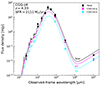 |
Fig. 3. FIR SED of the CGG-z4 integrated group galaxies. Photometry data are shown by circles with error bars or downward-pointing arrows for upper limits if S/N < 3. The magenta and cyan curves are the total SED scaled by the 870 μm flux of CGG-z4.a and CGG-z4.b, respectively. |
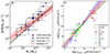 |
Fig. 4. Galaxy main sequence and brightness temperatures for the CGG-z4 galaxies. (a) SFR vs. stellar mass. The solid lines indicate the star-forming main sequence (MS) at z = 4.3, with the shaded area being the 1σ scatter (Speagle et al. 2014; Schreiber et al. 2015). CGG-z4.a and CGG-z4.b are shown as magenta diamonds, while other galaxies in CGG-z4 are shown as blue circles. (b) The brightness temperature relationship between [CI](1–0) and CO(4–3). CGG-z4.a and CGG-z4.b are shown as magenta diamonds. Linear fits are from Lee et al. (2021), with the data used being z = 2.5 protocluster galaxies from Lee et al. (2021) (L21). Cold dusty galaxies at z = 3.5 − 6 from Jin et al. (2019, 2022) (J19+22), a mix of local LIRGs (including AGNs), z = 1 main sequence galaxies, and DSFGs from Valentino et al. (2020) (V20), main sequence star-forming galaxies at z ∼ 1 from Boogaard et al. (2020) (B20), and the SPT DSFG average from Spilker et al. (2014) (S14). The remaining data comprise SMGs from Daddi et al. (2009), Cox et al. (2011), Lestrade et al. (2011), Alaghband-Zadeh et al. (2013), Aravena et al. (2013), Bothwell et al. (2013), Bothwell et al. (2017), Omont et al. (2013), Cañameras et al. (2015), Harrington et al. (2016), Yang et al. (2017), Valentino et al. (2020). |
4.5. Gas mass estimates
To estimate the gas mass from the dust emission in CGG-z4.a and CGG-z4.b, we used a 850 μm conversion from Dunne et al. (2022). The method was originally pioneered by Scoville et al. (2013, 2016), Genzel et al. (2015). They investigated a number of αX conversion factors by dividing their galaxy sample into two. The first group is extreme starburst “SMGs” containing the high-redshift sub-mm selected galaxies that were discovered pre-ALMA; as such, these are extreme star-forming systems (based on their detection), along with the local ULIRGs and some LIRGs that have evidence for being very intensely star-forming and obscured regions where conditions are likely to be extreme (Díaz-Santos et al. 2017; Falstad et al. 2021). The second group is main sequence galaxies that contain the lower luminosity local disc galaxies, along with the LIRGS (which are not extreme), intermediate redshift sources selected at 250 μm from the Herschel-ATLAS, z = 0.35 galaxies from Dunne et al. (2021) and the z < 0.3 VALES galaxies (Hughes et al. 2017), the z ∼ 1 galaxies (Valentino et al. 2018; Bourne et al. 2019), and the ASPECs sources denoted as “MS” in that survey (Boogaard et al. 2020). We refer to Table 1 in Dunne et al. (2022) for a full reference list.
We used an α850 value of  , such that M
 . L850 is calculated as follows

where DL is the luminosity distance, Sν(obs) is the observed flux density and K is the K-correction to rest-frame 850 μm, which is defined as
where νrest = νobs(1 + z), Td is the luminosity-weighted dust temperature, from an isothermal fit to the SED with the dust emissivity, β. Given their sub-mm brightness and the fact that they are optical/NIR dark, CGG-z4.a and CGG-z4.b are likely starbursts with optically thick dust emission. To account for this possibility, we performed a modified black body fitting using a thin- and thick-dust model following Lamperti et al. (2019). The values we found for the thin dust model are:  ,
,  ; for the thick dust model, these are:
  ,
,  . We note that using a higher β ≈ 1.9 for the power law continuum fit changes its value by (at most) 3.4% and does not change the value of any line fluxes at the level of precision reported in this paper. The resulting K corrections are Kthin = 4.8 ± 1.3 × 10⁻¹ and Kthick = 2.9 ± 1.1 × 10⁻³. By scaling the SCUBA-2 850 μm flux by the ALMA 870 μm flux for CGG-z4.a and CGG-z4.b, we find the following luminosities, L850,thin,a = 1.4 ± 0.4 × 1024 W Hz−1, L850,thin,b = 7.2 ± 2.3 × 10²³ W Hz−1, L850,thick,a = 9.0 ± 4.0 × 10²³ W Hz−1, and L850,thin,b = 4.3 ± 1.8 × 10²³ W Hz−1. The resulting gas masses are
 ![$ \rm log(M_{\mathrm{gas,thin,a}}\,\rm [M_{\odot}]) = 11.29^{+0.12}_{-0.16} $](/articles/aa/full_html/2025/02/aa51448-24/aa51448-24-eq19.gif) ,
, ![$ \rm log(M_{\mathrm{gas,thin,b}}\,\rm [M_{\odot}]) = 10.99^{+0.12}_{-0.17} $](/articles/aa/full_html/2025/02/aa51448-24/aa51448-24-eq20.gif) ,
, ![$ \rm log(M_{\mathrm{gas,thick,a}}\,\rm [M_{\odot}]) = 11.07^{+0.15}_{-0.24} $](/articles/aa/full_html/2025/02/aa51448-24/aa51448-24-eq21.gif) , and
, and ![$ \rm log(M_{\mathrm{gas,thick,a}}\,\rm [M_{\odot}]) = 10.77^{+0.15}_{-0.24} $](/articles/aa/full_html/2025/02/aa51448-24/aa51448-24-eq22.gif) . In combination with the stellar mass estimates, we can estimate the gas mass fraction Mgas/M⋆, with CGG-z4.a and CGG-z4.b having inferred gas mass fractions (estimated through Monte Carlo sampling) of
. In combination with the stellar mass estimates, we can estimate the gas mass fraction Mgas/M⋆, with CGG-z4.a and CGG-z4.b having inferred gas mass fractions (estimated through Monte Carlo sampling) of  and
and  using a thin dust model and
  and
and  using a thick dust model. The ratio Mgas/SFR approximates the gas depletion timescale, which is the inverse of the star formation efficiency (SFE). Given the gas mass and SFR of CGG-z4.a and CGG-z4.b both have gas depletion times of 140 ± (44,46) Myr using a thin dust model and 84 ± (36,37) Myr using a thick dust model. The thick dust model results in 0.22 dex lower gas masses, which, in turn, means that the gas mass factions and gas depletion times are 60% of the thin dust model values. For comparison, we used our available CO lines and an αCO conversion to estimate M
 . Since we did not have data for the CO(1–0) line, we instead converted the
  to
to  first. By comparing the flux ratio of CO(5–4) and CO(4–3) lines for CGG-z4.a and CGG-z4.b, we find that they have values of 1.52 ± 0.24 and 1.41 ± 0.36, which is close to the thermalization limit of
  (Narayanan & Krumholz 2014); therefore, we obtained the ratio rL′41 = L′CO(1 − 0)/L′CO(4 − 3) ∼ 1.0. We note that there is a systematic error in using a value of rL′41 = 1.0 that is unaccounted for. For the value of αCO, we used the canonical value for star-bursting high-z SMGs of
 ![$ \alpha_{\mathrm{CO}}=0.8\,\rm [M_{\odot}\, pc^{-2}\, (K\,km\, s^{-1})^{-1}] $](/articles/aa/full_html/2025/02/aa51448-24/aa51448-24-eq31.gif) (Downes & Solomon 1998; Tacconi et al. 2008; Carilli et al. 2010). Multiplying by a factor ×1.36 to account for the contribution from helium, this gives a gas mass of
(Downes & Solomon 1998; Tacconi et al. 2008; Carilli et al. 2010). Multiplying by a factor ×1.36 to account for the contribution from helium, this gives a gas mass of ![$ \rm log(M_{\mathrm{gas}}\,\rm [M_{\odot}]) = 10.51^{+0.04}_{-0.04} $](/articles/aa/full_html/2025/02/aa51448-24/aa51448-24-eq32.gif) and
and ![$ \rm log(M_{\mathrm{gas}}\,\rm [M_{\odot}]) = 10.28^{+0.05}_{-0.06} $](/articles/aa/full_html/2025/02/aa51448-24/aa51448-24-eq33.gif) for CGG-z4.a and CGG-z4.b, respectively. These values are ∼0.7, 0.5 dex lower than the ones estimated using the fit values and result in both lower gas mass ratio (
for CGG-z4.a and CGG-z4.b, respectively. These values are ∼0.7, 0.5 dex lower than the ones estimated using the fit values and result in both lower gas mass ratio ( and
and  ) and lower gas depletion times (23 ± 2 Myr and 27 ± 4 Myr).
It has been argued in recent times that there is no bimodality in the αCO value between star-bursting SMGs and main sequence galaxies as investigated in Dunne et al. (2022). Dunne et al. (2022) reported a value of ![$ \alpha_{\mathrm{CO}}=3.8\pm0.1 \,\rm [M_{\odot}\, pc^{-2}\, (K\,km\, s^{-1})^{-1}] $](/articles/aa/full_html/2025/02/aa51448-24/aa51448-24-eq36.gif) (including a factor 1.36 to account for He). Harrington et al. (2021) similarly found
(including a factor 1.36 to account for He). Harrington et al. (2021) similarly found ![$ \alpha_{\mathrm{CO}}=3.4{-}4.2 \,\rm [M_{\odot}\, pc^{-2}\, (K\, km\, s^{-1})^{-1}] $](/articles/aa/full_html/2025/02/aa51448-24/aa51448-24-eq37.gif) for lensed SMGs at z ∼ 1.0 − 3.5. Using the αCO value of Dunne et al. (2022), we obtained estimates for the gas mass:
for lensed SMGs at z ∼ 1.0 − 3.5. Using the αCO value of Dunne et al. (2022), we obtained estimates for the gas mass: ![$ \rm log(M_{\mathrm{gas}}\,\rm [M_{\odot}]) = 11.05^{+0.04}_{-0.04} $](/articles/aa/full_html/2025/02/aa51448-24/aa51448-24-eq38.gif) and
and ![$ \rm log(M_{\mathrm{gas}}\,\rm [M_{\odot}]) = 10.82^{+0.05}_{-0.06} $](/articles/aa/full_html/2025/02/aa51448-24/aa51448-24-eq39.gif) for CGG-z4.a and CGG-z4.b. Compared to the two dust models, these estimates are closer to the ones using the thick dust model, though the 1σ errors overlap with both dust models. The gas mass ratios for CGG-z4.a and CGG-z4.b are
for CGG-z4.a and CGG-z4.b. Compared to the two dust models, these estimates are closer to the ones using the thick dust model, though the 1σ errors overlap with both dust models. The gas mass ratios for CGG-z4.a and CGG-z4.b are  and
and  and gas depletion times are 80 ± 9 Myr and 94 ± 15 Myr, respectively. Lastly, we can estimate the gas mass from the
  $](/articles/aa/full_html/2025/02/aa51448-24/aa51448-24-eq42.gif) line following Dunne et al. (2022), giving us a value of
line following Dunne et al. (2022), giving us a value of ![$ \alpha_{\mathrm{CI}}=16.2 \pm 0.4 \,\rm [M_{\odot}\, pc^{-2}\, (K\,km\, s^{-1})^{-1}] $](/articles/aa/full_html/2025/02/aa51448-24/aa51448-24-eq43.gif) for SMGs. We used the 2σ upper limit for CGG-z4.b. We estimated the gas masses for CGG-z4.a and CGG-z4.b as
for SMGs. We used the 2σ upper limit for CGG-z4.b. We estimated the gas masses for CGG-z4.a and CGG-z4.b as ![$ \rm log(M_{\mathrm{gas}}\,\rm [M_{\odot}]) = 11.14^{+0.09}_{-0.11} $](/articles/aa/full_html/2025/02/aa51448-24/aa51448-24-eq44.gif) and
and ![$ \rm log(M_{\mathrm{gas}}\,\rm [M_{\odot}]) < 10.66 $](/articles/aa/full_html/2025/02/aa51448-24/aa51448-24-eq45.gif) . We note that using Eq. (8) in Dunne et al. (2022) also gives consistent results for the gas mass. This results in gas mass ratios of
. We note that using Eq. (8) in Dunne et al. (2022) also gives consistent results for the gas mass. This results in gas mass ratios of  and < 2.3 and gas depletion times of 99 ± 23 Myr and < 69 Myr, respectively. The estimate for CGG-z4.a is in agreement with the ones using the two dust models (with the thick dust model being closer) and an
 ![$ \alpha_{\mathrm{CO}}=3.8 \,\rm [M_{\odot}\, pc^{-2}\, (K\,km\, s^{-1})^{-1}] $](/articles/aa/full_html/2025/02/aa51448-24/aa51448-24-eq47.gif) ; whereas for CGG-z4.b, the upper limit is in a good general agreement with all the other estimates.
; whereas for CGG-z4.b, the upper limit is in a good general agreement with all the other estimates.
A summary of the different estimates is given in Table D.1. Apart from the upper limit based on using  $](/articles/aa/full_html/2025/02/aa51448-24/aa51448-24-eq48.gif) , the ratio between the objects is consistent, with the gas mass ratio and gas depletion times essentially being the same. To constrain the estimates of Mgas better, observations of the 115 GHz CO(1–0) line are needed.
, the ratio between the objects is consistent, with the gas mass ratio and gas depletion times essentially being the same. To constrain the estimates of Mgas better, observations of the 115 GHz CO(1–0) line are needed.
5. Discussion
5.1. Line ratios and ISM conditions
To investigate the physical state of CGG-z4.a and CGG-z4.b, we compare their available line ratios with public data from different types of sources. The literature sources include luminous IR galaxies (LIRGs) from Lu et al. (2017), star-forming galaxies (SFGs) from Valentino et al. (2020), SMGs from Bothwell et al. (2017), Valentino et al. (2020), QSOs from Barvainis et al. (1997), Pety et al. (2004). Figure 5 shows the relationship between the flux ratios of r![$ _{\mathrm{[CI]10/CO43}}=[\rm C_{\mathrm{I}}](1{-}0)/CO(4{-}3) $](/articles/aa/full_html/2025/02/aa51448-24/aa51448-24-eq49.gif) and r
and r . The ratio r[CI]10/CO43 is a proxy for the ratio between the amount of total gas present in the galaxy and the amount of dense gas present to form stars, which, in turn, means it is indicative of the ratio between the total gas mass and the SFR. The low values of rCI43 for CGG-z4.a,b are consistent with our low estimates for the gas depletion time of the galaxies. The values of rCI43 are close to the ones that are lowest in our reference sample; namely, the two quasars Cloverleaf (Barvainis et al. 1997) and PSS-2322+1944 (Pety et al. 2004). However, in the case of these quasars, the detectability of molecular and neutral atomic transitions is in large part due to the high emissivity of the gas and magnification from gravitational lensing, as opposed to a high (dense) gas mass. The r54 ratio describes the excitation state of the galaxies. However, we note that to fully characterize the galaxies, a full CO SLED should be constructed. CGG-z4.a and CGG-z4.b have relatively high values of r54, close to the 1.56 limit for a fully thermalized gas. The high values of r54 can indicate different gas conditions in the two galaxies, such as high temperatures, high densities, and/or high pressures.
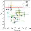 |
Fig. 5. Flux ratios of r[CI]10/CO43 and r54. The thermalization limit for r54 is given by |
We further attempted to investigate the gas density using a PDR model. The PDR model combines available line ratios to constrain the radiation field intensity and the hydrogen nucleus volume density. To constrain the PDR model, typically three line ratios are needed. Utilizing the Python package photodissociation region toolbox (pdrtpy, Pound & Wolfire 2023), we found the Wolfire-Kaufman 2006 model (Kaufman et al. 2006), with a constant density and solar metallicity, to have three available line ratios: r[CI]10/CO43, r[CI]10/CO54, and r[CI]10/IFIR. Here,  is the total FIR intensity, which we have access to from the SED fitting, and (as with the SFR) we scaled to CGG-z4.a and CGG-z4.b using their ALMA 870 μm flux. We determine a value from the full SED of
  . The package was run using the built-in emcee Markov chain Monto Carlo sampler (Foreman-Mackey et al. 2013), with 2000 steps and 200 walkers to sample the posterior distribution for the model parameters. For CGG-z4.a, the density is
  and radiation field
  Habing (the local Galactic interstellar radiation field, which has a value of 1.6 × 10⁻⁶ W m−2). For CGG-z4.b, we only have an upper limit available for the [CI](1–0) line and therefore the pdr models are poorly constrained. Given the available models, we can determine that
  and G0 > 10.0 Habing.
To make a comparison with SMGs in the literature, we used a wavelength range of 42.5 − 122.5 μm in the rest-frame (Wardlow et al. 2017) and determined  . We obtained
  ,
,  Habing for CGG-z4.a and
  and G0 > 6.0 Habing for CGG-z4.b. Compared to the SMGs in Wardlow et al. (2017), which have densities of
  and intensities of
  Habing, CGG-z4.a has a similar density and an intensity that is slightly below their sample. It should be noted that the Wardlow et al. (2017) sample mainly consists of z = 1 − 3 galaxies. Their lensed galaxy G15v2.779 at z = 4.243 has the closest redshift to CGG-z4.a, which shows a similar
  of 2.93 × 10⁻¹⁶ W m−2 after a correction for magnification.
5.2. Gas depletion times
To compare the efficiency with which these galaxies form stars to test if CGG-z4.a and CCG-z4.b differ from both other SMGs and field galaxies, we compared the depletion times of the CCG-z4 galaxies with those from SPT2349-56 and the sample of z > 4 SMGs of Jin et al. (2019, 2022). We compared these to the scaling relations of field samples Scoville et al. (2017), Tacconi et al. (2018), Liu et al. (2019), Kokorev et al. (2021), normalized to a redshift of z = 4.3 and log(M⋆ [Ṁ]) = 10.67 (the average stellar mass of CGG-z4.a and CGG-z4.b). We use the gas depletion times estimated using the [CI](1–0) line for CGG-z4.a and CGG-z4.b, since it is the estimate least reliant on conversions that could have systematic uncertainties, such as the choice of dust model or the conversion from CO(4–3) to CO(1–0). From Fig. 6, we see that the CGG-z4.a and CGG-z4.b both have low depletion times (high SFEs) and are above the main sequence, being slightly below the field relation at z = 4.3. CGG-z4.b appears to be more offset from the field relations than CGG-z4.a, with both being closest to the relations from Scoville et al. (2017) and Tacconi et al. (2020). When comparing with the galaxies of Jin et al. (2019, 2022), they appear to be following the field relation, being similarly offset from the galaxy main sequence as CGG-z4.a and CGG-z4.b and having higher gas depletion times. The GN20 protocluster galaxies follow the field relation and are close to the ones from Jin et al. (2019, 2022); however, it is worth noting that their gas masses were calculated using an αCO derived from a gas-to-dust mass ratio method and dynamical modeling, which differs for each object. Compared to the galaxies of SPT2349-56, both CGG-z4.a and CGG-z4.b have similar depletion times, but the galaxies of SPT2349-56 are less offset from the main sequence; therefore, they appear offset from the field relations. This offset to the field relation can be explained by multiple factors. First, the gas mass used to calculate the depletion times was estimated using a αCO numerical value of 1.0 and taken from Hill et al. (2020), where they argued in favor of the use of this value for the sake of simplicity. Since they have a mix of the main sequence and starburst galaxies, it is possible that some of them should instead be using a αCO numerical value of ∼4 (or even higher) due to the low metallicity of main sequence galaxies at high-z (i.e., the evolution of mass-metallicity relation and the dependence of αCO versus metallicity), which would place the galaxies closer to the field relations. Secondly, it is possible that the stellar masses of Hill et al. (2020) could have a large uncertainty due to such factors as the unknown IMF and metallicity. Therefore, these values could be overestimated, resulting in an overly low offset from the Speagle et al. (2014) main sequence.
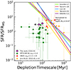 |
Fig. 6. Offset to the Speagle et al. (2014) galaxy main sequence vs. gas depletion time in Myr. The solid lines indicate the scaling relations of Scoville et al. (2017), Tacconi et al. (2018, 2020), Liu et al. (2019), Kokorev et al. (2021) normalized to z = 4.3 and log(M⋆ [Ṁ]) = 10.67. CGG-z4.a and CGG-z4.b are shown as magenta diamonds, SPT2349-56 galaxies are shown as green squares (Miller et al. 2018; Hill et al. 2020, 2022), GN20 galaxies are shown as red circles (Tan et al. 2014), and the Jin et al. (2019, 2022) galaxies are shown as orange diamonds. Depletion timescales were calculated for the SPT2349-56 galaxies using a gas mass with an αCO = 1.0 and a CO(4–3)/CO(1–0) line ratio r41 = 0.6 ± 0.05 (Spilker et al. 2014). The gas masses of each GN20 galaxy were calculated using the average of αCO derived from the gas-to-dust mass ratio method and dynamical modeling. The gas masses for the galaxies of Jin et al. (2019, 2022) were estimated from [CI](1–0) line data in each paper. |
5.3. Onset of quenching
With the low gas depletion times (high SFE), on the order of ∼ 100 Myr for the two dusty galaxies in CCG-z4, it is possible that they will become quiescent at z ∼ 4.0. Under the assumption that their SFE is constant, all the gas is converted into stars, and there is no gas replenishment, their final stellar masses would be ∼ 1011 M⊙ (with some variation, depending on the gas estimate used). This stellar mass is consistent with that of the massive quiescent galaxies in z > 3 dense environments (Kubo et al. 2021, 2022; McConachie et al. 2022; Jin et al. 2024a). For comparison, the large-scale structure Cosmic Vine (Jin et al. 2024a) at z = 3.44 contains two massive quiescent galaxies with stellar masses close to 1011 M⊙, and with star-formation histories from SED fitting suggesting they were quenched at 4 < z < 6. The fact that one of these massive galaxies has formed outside the protocluster core region disfavors environmental quenching with the prerequisite of a virialized cluster core. Jin et al. (2024a) argued that it is likely the two galaxies were quenched by merger-triggered starbursts in the past 500 Myr. In comparison, CGG-z4.a and CGG-z4.b are still in their starbursting phase at z = 4.33. The time between z = 4.33 and z = 4.0 is ≈ 140 Myr, and given their short gas depletion times it is possible for the CGG-z4 to evolve into galaxies similar to those of the Cosmic Vine. Due to the CGG-z4 galaxies’ optical/NIR dark nature, it is difficult to ascertain the morphology of the galaxies and comment on whether the galaxies have undergone a merger, similar to what is observed with galaxy A in the Cosmic Vine, where a compact bulge and tidal tail has been observed, both servings as indicators of a merger. Studying the morphology of the CGG-z4 optical/NIR galaxies would require deeper photometry than what is currently available in this part of the COSMOS field.
5.4. Comparison with literature samples
Here, we consider how CGG-z4 compares to other compact galaxy groups in the literature. As a compact galaxy group at z ∼ 5.2 (Jin et al. 2023), CGG-z5 has six members within a projected area of 1.5″ × 3″ (10 × 20 kpc2), which is more compact compared to the 13 members of CGG-z4 that are over a projected area of 13″ × 31″ (89 × 209 kpc2). The galaxies of CGG-z5 have low stellar masses and SFRs, which is in line with the low mass and low SFR galaxies in CGG-z4. The galaxies of CGG-z5 also appear to have lower AV’s (≈0.38), higher metallicities (≈0.54 Z⊙), and slightly higher ages (≈0.14 Gyr) to those in CGG-z4. CGG-z5 is expected to merge and grow into a log(M/M⊙) ∼ 10.7 galaxy at z ∼ 4 with a merging timescale of ∼ 400 Myr when comparing with similar galaxies to CGG-z5 in the EAGLE simulation (Crain et al. 2015; Schaye et al. 2015).
The compact group HPC1001 at z = 3.61 (Sillassen et al. 2022) has a similar total mass and ∼1/3 the SFR to CGG-z4, but a higher number density, with ten total members and eight members within 10″ × 10″ (70 × 70 kpc2). Comparing the most massive galaxy in the group, HPC1001.b (with a mass of 1011 M⊙) to CGG-z4.a and CGG-z4.b, it is placed ×3 below the main sequence at z = 3.7; whereas the two galaxies in CGG-z4 are ×6 and ×4.5 above the main sequence, respectively, at z = 4.3. Utilizing a dust-to-gas mass ratio of 1:100, HPC1001.b has a gas mass ratio of Mgas/M⋆ = 0.2 ± 0.1. Nonetheless, their gas depletion timescales are comparable, 200 Myr for HPC1001.b and ≈ 100 Myr for the CGG-z4 galaxies, with some variation depending on the method used, with the exception being the method using a αCO numerical value of 0.8.
A group that appears to have similar galaxies to CGG-z4 is the star-bursting galaxy group AzTEC5 at z ∼ 3.6 containing four members within 5″ × 5″ (35 × 35 kpc2, Gómez-Guijarro et al. 2018). AzTEC5-1,2 have ALMA 870 μm counterparts with SFRs and dust masses on a similar level to CGG-z4.a,b, with the ratio between the two galaxy pairs even being similar. Given that the stellar mass of CGG-z4.b is likely overestimated, the ratios of the stellar mass may also be similar; however, in the case of AzTEC5, it is the less actively star-forming galaxy AzTEC5-1 that has the higher stellar mass.
A protocluster found close to the redshift of CCG-z4 is GN20 at z = 4.05 (Tan et al. 2014). The structure contains the GN20 SMG, which is one of the brightest sources in the GOODS-N field, as well as two additional SMGs, GN20.2a and GN20.2b, located within ∼25″ (projected 170 kpc) of GN20. Much like CCG-z4, the GN20 galaxies are all starburst with large amounts of molecular gas surrounded by 14 B-band dropout galaxies within 25″ of GN20. Their gas depletion times are similar to CGG-z4 (at least when comparing their CO estimates of ∼ 200 Myr). While the CGG-z4 galaxies are optical/NIR dark, the GN20 galaxies do have counterparts, although they appear offset from the sub-mm emission.
We also compare CGG-z4 to the z = 4.3 protocluster SPT2349-56. The protocluster has a 130 kpc core region that contains 14 star-forming (total SFR ∼ 5000 M⊙ yr−1) and massive galaxies (M⋆ ∼ 1010 M⊙) (Miller et al. 2018; Hill et al. 2020, 2022). The size of the structure and number of sources in the core are comparable to CGG-z4, but the SPT sources are all highly star-forming and detected in either CO(4–3) or [CII] emission. The gas masses of CGG-z4.a and CGG-z4.b are slightly higher compared to the SPT galaxies, with ranges between 9.30 < log(Mgas [M⊙]) < 10.88, while the stellar masses are comparable with ranges between 10.08 < log(Mgas [M⊙]) < 11.35. While the gas mass ratios are generally lower for the SPT galaxies, ranging from 0.06 to 0.77, their gas depletion times are similar to the CGG-z4 galaxies, ranging from 43 Myr to 119 Myr.
5.5. Comparison with simulations
To understand how CGG-z4 would evolve with time, we compare it to massive structures in simulations with similar dark matter halo mass, log(MDM [M⊙]) = 12.8 ± 0.4. Comparing with the curves of Chiang et al. (2013) for the most massive progenitor of present-day clusters in a cluster halo merger tree, we find that CGG-z4 is expected to grow into a Virgo- or Coma-like cluster over the next 10 billion years. It should be noted that halo mass estimates can vary greatly between different models (compare the different estimates in Sect. 4.3) due to the different assumptions that go into estimating the dark matter halo mass. Given these caveats, a conservative prediction would be that CGG-z4 is likely to grow into a log(MDM [M⊙]) > 14.0 by z = 0. The presence of highly star-forming galaxies, with large amounts of dense gas in a compact environment, aligns with what we expect from a protocluster in its growing phase at z > 3 (Shimakawa et al. 2018). In the case that CGG-z4 will go on to form a galaxy cluster, we attempt to assess the fate of the two most massive galaxies, CGG-z4.a and CGG-z4.b, by making a comparison with the TNG300 simulation (Pillepich et al. 2018). Montenegro-Taborda et al. (2023) selected 280 systems with M200 > 1014 M⊙ at z = 0 in the TNG300 simulation and traced their progenitors and proto-BCGs at high redshift. Using the results of BCG progenitors by Montenegro-Taborda et al. (2023), the BCG stellar masses at z = 4.3 are expected to be on the order of ![$ \rm log(M_{\mathrm{BCG}}\,\rm [M_{\odot}]) = 10.5^{+0.7}_{-0.9} $](/articles/aa/full_html/2025/02/aa51448-24/aa51448-24-eq64.gif) , consistent with the stellar masses of CGG-z4.a and CGG-z4.b. On the other hand, the halo mass of CGG-z4 log(MDM [M⊙]) = 12.8 ± 0.4 is above the statistical mass
, consistent with the stellar masses of CGG-z4.a and CGG-z4.b. On the other hand, the halo mass of CGG-z4 log(MDM [M⊙]) = 12.8 ± 0.4 is above the statistical mass ![$ \rm log(M_{200}\,\rm [M_{\odot}]) = 12.3^{+0.3}_{-0.5} $](/articles/aa/full_html/2025/02/aa51448-24/aa51448-24-eq65.gif) of the clusters at z ∼ 4. These comparisons support the idea that CGG-z4.a and CGG-z4.b are BCGs undergoing formation in a massive cluster.
of the clusters at z ∼ 4. These comparisons support the idea that CGG-z4.a and CGG-z4.b are BCGs undergoing formation in a massive cluster.
6. Conclusions
Thanks to the use of ALMA and ancillary data in the COSMOS field, we have discovered a compact galaxy group, CGG-z4, hosting two optically/NIR dark galaxies at z = 4.3. We report the following conclusions:
-
CCG-z4 contains two optically/NIR dark galaxies with spectroscopic redshifts at z = 4.3 and 11 optical/NIR-detected candidate members, with photometric redshifts at 4.0 < z < 4.6. The galaxies are spread out over a projected area of 13″ × 31″ (89 × 209 kpc2).
-
The two optically/NIR dark galaxies, CGG-z4.a and CGG-z4.b, both have robust detections of CO(5–4) and CO(4–3) emission from ALMA 3 mm line scans. CGG-z4.a has a detection of [CI](1–0) emission, while CGG-z4.b has a detection of H2O(11, 0 − 10, 1) in absorption. We performed spectral stacking of all the optically/NIR-detected galaxies in CGG-z4 and found no definitive detection of spectral lines at the 2σ level.
-
Using dust continuum, CO, and CI lines as gas tracers, we found CGG-z4.a and CGG-z4.b are starburst galaxies with large amount of gas reservoirs (log(Mgas [M⊙]) ∼ 11.0), massive stellar masses (log(M⋆ [M⊙]) ∼ 10.7), and short gas depletion times (∼ 100 Myr).
-
We compared the line ratios of CGG-z4.a and CGG-z4.b with literature sample and found the ratio r54 is close to the thermalization, while rCI43 is among the lowest values compared to galaxies from the literature, indicating a high excitation of the ISM and efficient star formation.
-
The high SFEs in CGG-z4.a and CGG-z4.b suggest the onset of quenching. Assuming all of the gas reservoirs are converted to stars under the current SFR, these galaxies would grow ∼2× their stellar masses up to ∼ 1011 M⊙ and would enter a quiescent phase at z ∼ 4.0, which would be similar to massive quiescent galaxies found in other overdense structures at z > 3.
-
We used multiple approaches to estimate the dark matter halo mass of CGG-z4 and found a best estimate of log(MDM [M⊙]) = 12.8 ± 0.4. Comparisons with the simulations suggest that CGG-z4 is a forming protocluster, which is likely to form a cluster with M > 1014 M⊙ by z ∼ 0, and the two massive dusty galaxies will form BCGs in the cluster.
Spectroscopic follow-up of the nearby optically/NIR detected galaxies in CGG-z4 would further improve the completeness of the membership. JWST follow-up would also robustly constrain the stellar mass of optically/NIR dark galaxies, and further ALMA [CII] observations would be the key to unveiling the inter-group medium and allow us to assess the dynamic state of this structure.
Acknowledgments
The Cosmic Dawn Center (DAWN) is funded by the Danish National Research Foundation under grant No. 140. SJ and ML acknowledge the financial support from the European Union’s Horizon Europe research and innovation program under the Marie Skłodowska-Curie grant agreement No. 101060888 and 101107795. JH acknowledges support from the ERC Consolidator Grant 101088676 (VOYAJ). This paper makes use of the following ALMA data: ADS/JAO.ALMA#2016.1.00463.S, ADS/JAO.ALMA#2021.1.00246.S, ADS/JAO.ALMA#2022.1.00884.S. ALMA is a partnership of ESO (representing its member states), NSF (USA), and NINS (Japan), together with NRC (Canada), NSTC and ASIAA (Taiwan), and KASI (Republic of Korea), in cooperation with the Republic of Chile. The Joint ALMA Observatory is operated by ESO, AUI/NRAO and NAOJ. We acknowledge the following open-source software packages used in the analysis: Astropy (Astropy Collaboration 2013), Matplotlib (Hunter 2007), Numpy (Harris et al. 2020), Scipy (Virtanen et al. 2020), Uncertainties: a Python package for calculations with uncertainties, Eric O. Lebigot, http://pythonhosted.org/uncertainties/.
References
- Alaghband-Zadeh, S., Chapman, S. C., Swinbank, A. M., et al. 2013, MNRAS, 435, 1493 [Google Scholar]
- Algera, H. S. B., van der Vlugt, D., Hodge, J. A., et al. 2020, ApJ, 903, 139 [Google Scholar]
- Aravena, M., Murphy, E. J., Aguirre, J. E., et al. 2013, MNRAS, 433, 498 [NASA ADS] [CrossRef] [Google Scholar]
- Astropy Collaboration (Robitaille, T. P., et al.) 2013, A&A, 558, A33 [NASA ADS] [CrossRef] [EDP Sciences] [Google Scholar]
- Barrufet, L., Oesch, P. A., Weibel, A., et al. 2023, MNRAS, 522, 449 [NASA ADS] [CrossRef] [Google Scholar]
- Barvainis, R., Maloney, P., Antonucci, R., & Alloin, D. 1997, ApJ, 484, 695 [NASA ADS] [CrossRef] [Google Scholar]
- Behroozi, P. S., Wechsler, R. H., & Conroy, C. 2013, ApJ, 770, 57 [NASA ADS] [CrossRef] [Google Scholar]
- Benson, A. J., Borgani, S., De Lucia, G., Boylan-Kolchin, M., & Monaco, P. 2012, MNRAS, 419, 3590 [CrossRef] [Google Scholar]
- Boogaard, L. A., van der Werf, P., Weiss, A., et al. 2020, ApJ, 902, 109 [NASA ADS] [CrossRef] [Google Scholar]
- Bothwell, M. S., Smail, I., Chapman, S. C., et al. 2013, MNRAS, 429, 3047 [Google Scholar]
- Bothwell, M. S., Aguirre, J. E., Aravena, M., et al. 2017, MNRAS, 466, 2825 [Google Scholar]
- Bourne, N., Dunlop, J. S., Simpson, J. M., et al. 2019, MNRAS, 482, 3135 [Google Scholar]
- Brammer, G. B., van Dokkum, P. G., & Coppi, P. 2008, ApJ, 686, 1503 [Google Scholar]
- Brinch, M., Greve, T. R., Weaver, J. R., et al. 2023, ApJ, 943, 153 [NASA ADS] [CrossRef] [Google Scholar]
- Brinch, M., Greve, T. R., Sanders, D. B., et al. 2024, MNRAS, 527, 6591 [Google Scholar]
- Bruzual, G., & Charlot, S. 2003, MNRAS, 344, 1000 [NASA ADS] [CrossRef] [Google Scholar]
- Calvi, R., Castignani, G., & Dannerbauer, H. 2023, A&A, 678, A15 [NASA ADS] [CrossRef] [EDP Sciences] [Google Scholar]
- Cañameras, R., Nesvadba, N. P. H., Guery, D., et al. 2015, A&A, 581, A105 [Google Scholar]
- Capak, P. L., Riechers, D., Scoville, N. Z., et al. 2011, Nature, 470, 233 [Google Scholar]
- Carilli, C. L., Daddi, E., Riechers, D., et al. 2010, ApJ, 714, 1407 [NASA ADS] [CrossRef] [Google Scholar]
- Carnall, A. C., McLure, R. J., Dunlop, J. S., & Davé, R. 2018, MNRAS, 480, 4379 [Google Scholar]
- Carnall, A. C., Begley, R., McLeod, D. J., et al. 2023, MNRAS, 518, L45 [Google Scholar]
- Casey, C. M., Kartaltepe, J. S., Drakos, N. E., et al. 2023, ApJ, 954, 31 [NASA ADS] [CrossRef] [Google Scholar]
- Chabrier, G. 2003, PASP, 115, 763 [Google Scholar]
- Chiang, Y.-K., Overzier, R., & Gebhardt, K. 2013, ApJ, 779, 127 [Google Scholar]
- Chiang, Y.-K., Overzier, R. A., Gebhardt, K., & Henriques, B. 2017, ApJ, 844, L23 [Google Scholar]
- Claude, S., Jiang, F., Niranjanan, P., et al. 2006, in Seventeenth International Symposium on Space Terahertz Technology, eds. A. Hedden, M. Reese, D. Santavicca, et al., 154 [Google Scholar]
- Cooper, O. R., Casey, C. M., Zavala, J. A., et al. 2022, ApJ, 930, 32 [NASA ADS] [CrossRef] [Google Scholar]
- Cox, P., Krips, M., Neri, R., et al. 2011, ApJ, 740, 63 [NASA ADS] [CrossRef] [Google Scholar]
- Crain, R. A., Schaye, J., Bower, R. G., et al. 2015, MNRAS, 450, 1937 [NASA ADS] [CrossRef] [Google Scholar]
- Daddi, E., Dannerbauer, H., Stern, D., et al. 2009, ApJ, 694, 1517 [Google Scholar]
- Daddi, E., Valentino, F., Rich, R. M., et al. 2021, A&A, 649, A78 [NASA ADS] [CrossRef] [EDP Sciences] [Google Scholar]
- Daddi, E., Rich, R. M., Valentino, F., et al. 2022, ApJ, 926, L21 [NASA ADS] [CrossRef] [Google Scholar]
- Dannerbauer, H., Kurk, J. D., De Breuck, C., et al. 2014, A&A, 570, A55 [NASA ADS] [CrossRef] [EDP Sciences] [Google Scholar]
- Díaz-Santos, T., Armus, L., Charmandaris, V., et al. 2017, ApJ, 846, 32 [Google Scholar]
- Díaz-Santos, T., Assef, R. J., Blain, A. W., et al. 2018, Science, 362, 1034 [Google Scholar]
- Donevski, D., Lapi, A., Małek, K., et al. 2020, A&A, 644, A144 [NASA ADS] [CrossRef] [EDP Sciences] [Google Scholar]
- Downes, D., & Solomon, P. M. 1998, ApJ, 507, 615 [NASA ADS] [CrossRef] [Google Scholar]
- Draine, B. T., & Li, A. 2007, ApJ, 657, 810 [CrossRef] [Google Scholar]
- Dunne, L., Maddox, S. J., Vlahakis, C., & Gomez, H. L. 2021, MNRAS, 501, 2573 [NASA ADS] [CrossRef] [Google Scholar]
- Dunne, L., Maddox, S. J., Papadopoulos, P. P., Ivison, R. J., & Gomez, H. L. 2022, MNRAS, 517, 962 [NASA ADS] [CrossRef] [Google Scholar]
- Falstad, N., Aalto, S., König, S., et al. 2021, A&A, 649, A105 [NASA ADS] [CrossRef] [EDP Sciences] [Google Scholar]
- Foreman-Mackey, D., Hogg, D. W., Lang, D., & Goodman, J. 2013, PASP, 125, 306 [Google Scholar]
- Genzel, R., Tacconi, L. J., Lutz, D., et al. 2015, ApJ, 800, 20 [Google Scholar]
- Gildas Team 2013, Astrophysics Source Code Library [record ascl:1305.010] [Google Scholar]
- Ginolfi, M., Piconcelli, E., Zappacosta, L., et al. 2022, Nat. Commun., 13, 4574 [NASA ADS] [CrossRef] [Google Scholar]
- Gómez-Guijarro, C., Toft, S., Karim, A., et al. 2018, ApJ, 856, 121 [Google Scholar]
- Gómez-Guijarro, C., Elbaz, D., Xiao, M., et al. 2022, A&A, 658, A43 [NASA ADS] [CrossRef] [EDP Sciences] [Google Scholar]
- Gottumukkala, R., Barrufet, L., Oesch, P. A., et al. 2024, MNRAS, 530, 966 [NASA ADS] [CrossRef] [Google Scholar]
- Harikane, Y., Ouchi, M., Ono, Y., et al. 2019, ApJ, 883, 142 [Google Scholar]
- Harrington, K. C., Yun, M. S., Cybulski, R., et al. 2016, MNRAS, 458, 4383 [NASA ADS] [CrossRef] [Google Scholar]
- Harrington, K. C., Weiss, A., Yun, M. S., et al. 2021, ApJ, 908, 95 [NASA ADS] [CrossRef] [Google Scholar]
- Harris, C. R., Millman, K. J., van der Walt, S. J., et al. 2020, Nature, 585, 357 [NASA ADS] [CrossRef] [Google Scholar]
- Heintz, K. E., Giménez-Arteaga, C., Fujimoto, S., et al. 2023, ApJ, 944, L30 [NASA ADS] [CrossRef] [Google Scholar]
- Higdon, J. L., Higdon, S. J. U., Willner, S. P., et al. 2008, ApJ, 688, 885 [NASA ADS] [CrossRef] [Google Scholar]
- Hill, R., Chapman, S., Scott, D., et al. 2020, MNRAS, 495, 3124 [NASA ADS] [CrossRef] [Google Scholar]
- Hill, R., Chapman, S., Phadke, K. A., et al. 2022, MNRAS, 512, 4352 [NASA ADS] [CrossRef] [Google Scholar]
- Hirschmann, M., Naab, T., Somerville, R. S., Burkert, A., & Oser, L. 2012, MNRAS, 419, 3200 [CrossRef] [Google Scholar]
- Hopkins, P. F., Somerville, R. S., Cox, T. J., et al. 2009, MNRAS, 397, 802 [NASA ADS] [CrossRef] [Google Scholar]
- Hughes, T. M., Ibar, E., Villanueva, V., et al. 2017, MNRAS, 468, L103 [NASA ADS] [CrossRef] [Google Scholar]
- Hunter, J. D. 2007, Comput. Sci. Eng., 9, 90 [NASA ADS] [CrossRef] [Google Scholar]
- Jin, S., Daddi, E., Liu, D., et al. 2018, ApJ, 864, 56 [Google Scholar]
- Jin, S., Daddi, E., Magdis, G. E., et al. 2019, ApJ, 887, 144 [Google Scholar]
- Jin, S., Daddi, E., Magdis, G. E., et al. 2022, A&A, 665, A3 [NASA ADS] [CrossRef] [EDP Sciences] [Google Scholar]
- Jin, S., Sillassen, N. B., Magdis, G. E., et al. 2023, A&A, 670, L11 [NASA ADS] [CrossRef] [EDP Sciences] [Google Scholar]
- Jin, S., Sillassen, N. B., Magdis, G. E., et al. 2024a, A&A, 683, L4 [NASA ADS] [CrossRef] [EDP Sciences] [Google Scholar]
- Jin, S., Sillassen, N. B., Hodge, J., et al. 2024b, A&A, 690, L16 [NASA ADS] [CrossRef] [EDP Sciences] [Google Scholar]
- Jones, S. F., Blain, A. W., Assef, R. J., et al. 2017, MNRAS, 469, 4565 [Google Scholar]
- Kaufman, M. J., Wolfire, M. G., & Hollenbach, D. J. 2006, ApJ, 644, 283 [Google Scholar]
- Kennicutt, R. C., Jr. 1998, ARA&A, 36, 189 [Google Scholar]
- Kokorev, V. I., Magdis, G. E., Davidzon, I., et al. 2021, ApJ, 921, 40 [NASA ADS] [CrossRef] [Google Scholar]
- Kokorev, V., Jin, S., Magdis, G. E., et al. 2023, ApJ, 945, L25 [NASA ADS] [CrossRef] [Google Scholar]
- Kubo, M., Umehata, H., Matsuda, Y., et al. 2021, ApJ, 919, 6 [NASA ADS] [CrossRef] [Google Scholar]
- Kubo, M., Umehata, H., Matsuda, Y., et al. 2022, ApJ, 935, 89 [NASA ADS] [CrossRef] [Google Scholar]
- Laigle, C., McCracken, H. J., Ilbert, O., et al. 2016, ApJS, 224, 24 [Google Scholar]
- Lamperti, I., Saintonge, A., De Looze, I., et al. 2019, MNRAS, 489, 4389 [Google Scholar]
- Le Floc’h, E., Aussel, H., Ilbert, O., et al. 2009, ApJ, 703, 222 [Google Scholar]
- Lee, M. M., Tanaka, I., Iono, D., et al. 2021, ApJ, 909, 181 [NASA ADS] [CrossRef] [Google Scholar]
- Lestrade, J.-F., Carilli, C. L., Thanjavur, K., et al. 2011, ApJ, 739, L30 [NASA ADS] [CrossRef] [Google Scholar]
- Lewis, A. J. R., Ivison, R. J., Best, P. N., et al. 2018, ApJ, 862, 96 [NASA ADS] [CrossRef] [Google Scholar]
- Liu, D. 2020, Astrophysics Source Code Library [record ascl:2005.002] [Google Scholar]
- Liu, D., Daddi, E., Dickinson, M., et al. 2018, ApJ, 853, 172 [Google Scholar]
- Liu, D., Schinnerer, E., Groves, B., et al. 2019, ApJ, 887, 235 [Google Scholar]
- Liu, D., Daddi, E., Schinnerer, E., et al. 2021, ApJ, 909, 56 [NASA ADS] [CrossRef] [Google Scholar]
- Lu, N., Zhao, Y., Díaz-Santos, T., et al. 2017, ApJS, 230, 1 [Google Scholar]
- Lutz, D., Poglitsch, A., Altieri, B., et al. 2011, A&A, 532, A90 [NASA ADS] [CrossRef] [EDP Sciences] [Google Scholar]
- Magdis, G. E., Daddi, E., Béthermin, M., et al. 2012, ApJ, 760, 6 [NASA ADS] [CrossRef] [Google Scholar]
- Magnelli, B., Ivison, R. J., Lutz, D., et al. 2015, A&A, 573, A45 [NASA ADS] [CrossRef] [EDP Sciences] [Google Scholar]
- Mahieu, S., Lazareff, B., Maier, D., et al. 2005, Sixteenth International Symposium on Space Terahertz Technology, 99 [Google Scholar]
- Maier, D., Barbier, A., Lazareff, B., & Schuster, K. F. 2005, Sixteenth International Symposium on Space Terahertz Technology, 428 [Google Scholar]
- Marrone, D. P., Spilker, J. S., Hayward, C. C., et al. 2018, Nature, 553, 51 [NASA ADS] [CrossRef] [Google Scholar]
- McConachie, I., Wilson, G., Forrest, B., et al. 2022, ApJ, 926, 37 [NASA ADS] [CrossRef] [Google Scholar]
- McMullin, J. P., Waters, B., Schiebel, D., Young, W., & Golap, K. 2007, in Astronomical Data Analysis Software and Systems XVI, eds. R. A. Shaw, F. Hill, & D. J. Bell, Astronomical Society of the Pacific Conference Series, 376, 127 [Google Scholar]
- Miller, T. B., Chapman, S. C., Aravena, M., et al. 2018, Nature, 556, 469 [CrossRef] [Google Scholar]
- Montenegro-Taborda, D., Rodriguez-Gomez, V., Pillepich, A., et al. 2023, MNRAS, 521, 800 [NASA ADS] [CrossRef] [Google Scholar]
- Mullaney, J. R., Alexander, D. M., Goulding, A. D., & Hickox, R. C. 2011, MNRAS, 414, 1082 [Google Scholar]
- Muzzin, A., Marchesini, D., Stefanon, M., et al. 2013, ApJ, 777, 18 [NASA ADS] [CrossRef] [Google Scholar]
- Narayanan, D., & Krumholz, M. R. 2014, MNRAS, 442, 1411 [NASA ADS] [CrossRef] [Google Scholar]
- Newville, M., Stensitzki, T., Allen, D. B., & Ingargiola, A. 2014, https://doi.org/10.5281/zenodo.11813 [Google Scholar]
- Oke, J. B. 1974, ApJS, 27, 21 [Google Scholar]
- Oliver, S. J., Bock, J., Altieri, B., et al. 2012, MNRAS, 424, 1614 [NASA ADS] [CrossRef] [Google Scholar]
- Omont, A., Yang, C., Cox, P., et al. 2013, A&A, 551, A115 [NASA ADS] [CrossRef] [EDP Sciences] [Google Scholar]
- Oser, L., Ostriker, J. P., Naab, T., Johansson, P. H., & Burkert, A. 2010, ApJ, 725, 2312 [Google Scholar]
- Oteo, I., Ivison, R. J., Dunne, L., et al. 2018, ApJ, 856, 72 [Google Scholar]
- Overzier, R. A. 2016, A&ARv, 24, 14 [Google Scholar]
- Pety, J., Beelen, A., Cox, P., et al. 2004, A&A, 428, L21 [NASA ADS] [CrossRef] [EDP Sciences] [Google Scholar]
- Pillepich, A., Nelson, D., Hernquist, L., et al. 2018, MNRAS, 475, 648 [Google Scholar]
- Pound, M. W., & Wolfire, M. G. 2023, AJ, 165, 25 [NASA ADS] [CrossRef] [Google Scholar]
- Riechers, D. A., Weiss, A., Walter, F., et al. 2022, Nature, 602, 58 [NASA ADS] [CrossRef] [Google Scholar]
- Salim, S., Boquien, M., & Lee, J. C. 2018, ApJ, 859, 11 [Google Scholar]
- Schaye, J., Crain, R. A., Bower, R. G., et al. 2015, MNRAS, 446, 521 [Google Scholar]
- Schlafly, E. F., & Finkbeiner, D. P. 2011, ApJ, 737, 103 [Google Scholar]
- Schmidt, M. 1959, ApJ, 129, 243 [NASA ADS] [CrossRef] [Google Scholar]
- Schreiber, C., Pannella, M., Elbaz, D., et al. 2015, A&A, 575, A74 [NASA ADS] [CrossRef] [EDP Sciences] [Google Scholar]
- Scoville, N., Arnouts, S., Aussel, H., et al. 2013, ApJS, 206, 3 [Google Scholar]
- Scoville, N., Sheth, K., Aussel, H., et al. 2016, ApJ, 820, 83 [Google Scholar]
- Scoville, N., Lee, N., Vanden Bout, P., et al. 2017, ApJ, 837, 150 [Google Scholar]
- Shimakawa, R., Koyama, Y., Röttgering, H. J. A., et al. 2018, MNRAS, 481, 5630 [NASA ADS] [CrossRef] [Google Scholar]
- Shu, X., Yang, L., Liu, D., et al. 2022, ApJ, 926, 155 [NASA ADS] [CrossRef] [Google Scholar]
- Shuntov, M., McCracken, H. J., Gavazzi, R., et al. 2022, A&A, 664, A61 [NASA ADS] [CrossRef] [EDP Sciences] [Google Scholar]
- Sillassen, N. B., Jin, S., Magdis, G. E., et al. 2022, A&A, 665, L7 [NASA ADS] [CrossRef] [EDP Sciences] [Google Scholar]
- Sillassen, N. B., Jin, S., Magdis, G. E., et al. 2024, A&A, 690, A55 [NASA ADS] [CrossRef] [EDP Sciences] [Google Scholar]
- Simpson, J. M., Smail, I., Swinbank, A. M., et al. 2019, ApJ, 880, 43 [NASA ADS] [CrossRef] [Google Scholar]
- Smail, I., Morrison, G., Gray, M. E., et al. 1999, ApJ, 525, 609 [NASA ADS] [CrossRef] [Google Scholar]
- Smail, I., Dudzevičiūtė, U., Stach, S. M., et al. 2021, MNRAS, 502, 3426 [NASA ADS] [CrossRef] [Google Scholar]
- Smolčić, V., Novak, M., Bondi, M., et al. 2017, A&A, 602, A1 [Google Scholar]
- Speagle, J. S., Steinhardt, C. L., Capak, P. L., & Silverman, J. D. 2014, ApJS, 214, 15 [Google Scholar]
- Spilker, J. S., Marrone, D. P., Aguirre, J. E., et al. 2014, ApJ, 785, 149 [NASA ADS] [CrossRef] [Google Scholar]
- Springel, V., White, S. D. M., Jenkins, A., et al. 2005, Nature, 435, 629 [Google Scholar]
- Tacconi, L. J., Genzel, R., Smail, I., et al. 2008, ApJ, 680, 246 [Google Scholar]
- Tacconi, L. J., Genzel, R., Saintonge, A., et al. 2018, ApJ, 853, 179 [Google Scholar]
- Tacconi, L. J., Genzel, R., & Sternberg, A. 2020, ARA&A, 58, 157 [NASA ADS] [CrossRef] [Google Scholar]
- Talia, M., Cimatti, A., Giulietti, M., et al. 2021, ApJ, 909, 23 [NASA ADS] [CrossRef] [Google Scholar]
- Tan, Q., Daddi, E., Magdis, G., et al. 2014, A&A, 569, A98 [NASA ADS] [CrossRef] [EDP Sciences] [Google Scholar]
- Valentino, F., Magdis, G. E., Daddi, E., et al. 2018, ApJ, 869, 27 [Google Scholar]
- Valentino, F., Magdis, G. E., Daddi, E., et al. 2020, ApJ, 890, 24 [Google Scholar]
- van der Burg, R. F. J., Muzzin, A., Hoekstra, H., et al. 2014, A&A, 561, A79 [NASA ADS] [CrossRef] [EDP Sciences] [Google Scholar]
- van der Vlugt, D., Hodge, J. A., Jin, S., et al. 2023, ApJ, 951, 131 [NASA ADS] [CrossRef] [Google Scholar]
- Virtanen, P., Gommers, R., Oliphant, T. E., et al. 2020, Nat. Methods, 17, 261 [Google Scholar]
- Walter, F., Decarli, R., Carilli, C., et al. 2012, Nature, 486, 233 [Google Scholar]
- Wang, T., Elbaz, D., Daddi, E., et al. 2016, ApJ, 828, 56 [NASA ADS] [CrossRef] [Google Scholar]
- Wang, T., Schreiber, C., Elbaz, D., et al. 2019, Nature, 572, 211 [Google Scholar]
- Wardlow, J. L., Cooray, A., Osage, W., et al. 2017, ApJ, 837, 12 [NASA ADS] [CrossRef] [Google Scholar]
- Weaver, J. R., Kauffmann, O. B., Ilbert, O., et al. 2022, ApJS, 258, 11 [NASA ADS] [CrossRef] [Google Scholar]
- Xiao, M. Y., Elbaz, D., Gómez-Guijarro, C., et al. 2023, A&A, 672, A18 [NASA ADS] [CrossRef] [EDP Sciences] [Google Scholar]
- Yang, C., Omont, A., Beelen, A., et al. 2017, A&A, 608, A144 [NASA ADS] [CrossRef] [EDP Sciences] [Google Scholar]
- Zhou, L., Wang, T., Daddi, E., et al. 2024, A&A, 684, A196 [NASA ADS] [CrossRef] [EDP Sciences] [Google Scholar]
Appendix A: Photometry used for combined SED fitting of CGG-z4.a+b
Data used for SED fitting of CGG-z4.a,b.
Appendix B: Bagpipes SED fits
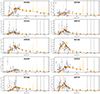 |
Fig. B.1. Bagpipes SED fits of the optical/NIR detected galaxies in CGG-z4. SEDs were fit at z = 4.331, the redshift of CGG-z4.a. |
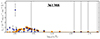 |
Fig. B.1. Continued. |
Appendix C: Galaxy properties from SED fitting
SED fitting result for CGG-z4 group galaxies.
Appendix D: Gas mass estimates and their products
Gas mass estimates for CGG-z4.a,b, and the products calculated from them.
All Tables
All Figures
|
Fig. 1. Images and spectra highlighting the member galaxies of the CGG-z4 galaxy group. Top left: VISTA Ks images overlaid with cyan SCUBA-2 850 μm contours in steps of 3, 5 and 7σ. Photometric redshift candidate members in the range 4.0 < z < 4.6 are highlighted with red dashed circles. Galaxies with ALMA continuum detections are highlighted as magenta-dashed circles. The green square highlights the region of the right image. Top right: VISTA RGB color images of CGG-z4 at z ∼ 4.3 using the Ks (red), J (green), and i (blue) bands. Two spectroscopically confirmed galaxies have ALMA 3 mm and 870 μm continuum emission shown as green and yellow contours. Contours are shown at levels 5, 7, and 10σ. ALMA beam sizes and an image scale are shown in the lower right corner. The RGB frames are composed using linear scales with identical limits. Bottom: ALMA 3 mm spectra for galaxies with emission line detections. The detected lines are highlighted in yellow with their names labeled. The red line shows Gaussian fits to the CO emission lines and a power law fit to the continuum that increases with frequency following the expression ν3.7. |
| In the text | |
|
Fig. 2. ALMA line and continuum maps, with black lines showing the positive contours and white dashed lines the negative contours, both starting from 2σ to 6σ in steps of 2σ; except for the continuum map, where the contours start from 3σ to 12σ with 3σ steps. The size and orientation of the beam are indicated in the lower left corner in red. Magenta crosses mark COSMOS2020 sources. |
| In the text | |
|
Fig. 3. FIR SED of the CGG-z4 integrated group galaxies. Photometry data are shown by circles with error bars or downward-pointing arrows for upper limits if S/N < 3. The magenta and cyan curves are the total SED scaled by the 870 μm flux of CGG-z4.a and CGG-z4.b, respectively. |
| In the text | |
|
Fig. 4. Galaxy main sequence and brightness temperatures for the CGG-z4 galaxies. (a) SFR vs. stellar mass. The solid lines indicate the star-forming main sequence (MS) at z = 4.3, with the shaded area being the 1σ scatter (Speagle et al. 2014; Schreiber et al. 2015). CGG-z4.a and CGG-z4.b are shown as magenta diamonds, while other galaxies in CGG-z4 are shown as blue circles. (b) The brightness temperature relationship between [CI](1–0) and CO(4–3). CGG-z4.a and CGG-z4.b are shown as magenta diamonds. Linear fits are from Lee et al. (2021), with the data used being z = 2.5 protocluster galaxies from Lee et al. (2021) (L21). Cold dusty galaxies at z = 3.5 − 6 from Jin et al. (2019, 2022) (J19+22), a mix of local LIRGs (including AGNs), z = 1 main sequence galaxies, and DSFGs from Valentino et al. (2020) (V20), main sequence star-forming galaxies at z ∼ 1 from Boogaard et al. (2020) (B20), and the SPT DSFG average from Spilker et al. (2014) (S14). The remaining data comprise SMGs from Daddi et al. (2009), Cox et al. (2011), Lestrade et al. (2011), Alaghband-Zadeh et al. (2013), Aravena et al. (2013), Bothwell et al. (2013), Bothwell et al. (2017), Omont et al. (2013), Cañameras et al. (2015), Harrington et al. (2016), Yang et al. (2017), Valentino et al. (2020). |
| In the text | |
|
Fig. 5. Flux ratios of r[CI]10/CO43 and r54. The thermalization limit for r54 is given by |
| In the text | |
|
Fig. 6. Offset to the Speagle et al. (2014) galaxy main sequence vs. gas depletion time in Myr. The solid lines indicate the scaling relations of Scoville et al. (2017), Tacconi et al. (2018, 2020), Liu et al. (2019), Kokorev et al. (2021) normalized to z = 4.3 and log(M⋆ [Ṁ]) = 10.67. CGG-z4.a and CGG-z4.b are shown as magenta diamonds, SPT2349-56 galaxies are shown as green squares (Miller et al. 2018; Hill et al. 2020, 2022), GN20 galaxies are shown as red circles (Tan et al. 2014), and the Jin et al. (2019, 2022) galaxies are shown as orange diamonds. Depletion timescales were calculated for the SPT2349-56 galaxies using a gas mass with an αCO = 1.0 and a CO(4–3)/CO(1–0) line ratio r41 = 0.6 ± 0.05 (Spilker et al. 2014). The gas masses of each GN20 galaxy were calculated using the average of αCO derived from the gas-to-dust mass ratio method and dynamical modeling. The gas masses for the galaxies of Jin et al. (2019, 2022) were estimated from [CI](1–0) line data in each paper. |
| In the text | |
|
Fig. B.1. Bagpipes SED fits of the optical/NIR detected galaxies in CGG-z4. SEDs were fit at z = 4.331, the redshift of CGG-z4.a. |
| In the text | |
|
Fig. B.1. Continued. |
| In the text | |
Current usage metrics show cumulative count of Article Views (full-text article views including HTML views, PDF and ePub downloads, according to the available data) and Abstracts Views on Vision4Press platform.
Data correspond to usage on the plateform after 2015. The current usage metrics is available 48-96 hours after online publication and is updated daily on week days.
Initial download of the metrics may take a while.