| Issue |
A&A
Volume 689, September 2024
|
|
|---|---|---|
| Article Number | A218 | |
| Number of page(s) | 11 | |
| Section | Cosmology (including clusters of galaxies) | |
| DOI | https://doi.org/10.1051/0004-6361/202450697 | |
| Published online | 13 September 2024 | |
Ultra-low-frequency LOFAR spectral indices of cluster radio halos
1
INAF – Istituto di Radioastronomia, via P. Gobetti 101, 40129
Bologna, Italy
2
Hamburger Sternwarte, Universität Hamburg, Gojenbergsweg 112, 21029
Hamburg, Germany
3
Leiden Observatory, Leiden University, PO Box 9513, 2300 RA
Leiden, The Netherlands
4
Dipartimento di Fisica e Astronomia, Università di Bologna, Via P. Gobetti 93/2, 40129
Bologna, Italy
5
ASTRON, the Netherlands Institute for Radio Astronomy, Oude Hoogeveensedijk 4, 7991 PD
Dwingeloo, The Netherlands
6
Department of Physics, Informatics and Mathematics, University of Modena and Reggio Emilia, 41125
Modena, Italy
7
Department of Physics, Astronomy and Mathematics, University of Hertfordshire, College Lane, Hatfield, AL10 9AB
UK
8
GEPI & ORN, Observatoire de Paris, Université PSL, CNRS, 5 Place Jules Janssen, 92190
Meudon, France
9
Department of Physics & Electronics, Rhodes University, PO Box 94, Grahamstown, 6140
South Africa
Received:
13
May
2024
Accepted:
17
June
2024
Context. A fraction of galaxy clusters harbor diffuse radio sources known as radio halos. The prevailing theory regarding their formation is based on second-order Fermi reacceleration of seed electrons caused by merger-driven turbulence in the intra-cluster medium. This mechanism is expected to be inefficient, which implies that a significant fraction of halos should have very steep energy spectra (α < −1.5).
Aims. We start investigating the potential and current limitations of the combination of the two surveys conducted by LOFAR, LoTSS (144 MHz) and LoLSS (54 MHz), to probe the origin of radio halos.
Methods. We followed up the 20 radio halos detected in Data Release 1 of LoTSS, which covers the HETDEX field, with the LoLSS survey, and we studied their spectral properties between 54 and 144 MHz.
Results. After removing compact sources, nine halos were excluded due to unreliable halo flux density measurements at 54 MHz. Our main finding is that 7 out of 11 (∼64%) exhibit an ultra-steep spectrum (α < −1.5), which is a key prediction of turbulent reacceleration models. We also note a tentative trend for more massive systems to host flatter halos, although the currently poor statistics do not allow for a deeper analysis.
Conclusions. Our sample suffers from low angular resolution at 54 MHz, which limits the accuracy of the compact-source subtraction. Nevertheless, this study is the first step toward providing compelling evidence for the existence of a large fraction of radio halos with a very steep spectrum, which is a fundamental prediction of turbulent reacceleration models. In this regard, the forthcoming second data release of LoLSS, along with the integration of LOFAR international stations and the instrumental upgrade to LOFAR2.0, will improve both the statistics and the low-frequency angular resolution, allowing us to determine the origin of radio halos in galaxy clusters conclusively.
Key words: instrumentation: interferometers / galaxies: clusters: general
© The Authors 2024
 Open Access article, published by EDP Sciences, under the terms of the Creative Commons Attribution License (https://creativecommons.org/licenses/by/4.0), which permits unrestricted use, distribution, and reproduction in any medium, provided the original work is properly cited.
This article is published in open access under the Subscribe to Open model. Subscribe to A&A to support open access publication.
1. Introduction
Radio halos are diffuse sources observed in the central regions of disturbed galaxy clusters (Willson 1970; van Weeren et al. 2019). They trace synchrotron emission by relativistic cosmic-ray (CR) electrons in the presence of magnetic fields in the intra-cluster medium (ICM, Brüggen et al. 2012; Brunetti & Jones 2014), the hot (∼107 − 108 K) plasma that permeates galaxy clusters. The synchrotron spectrum of radio halos can be described to a first approximation by a power-law, Sν ∝ να, with Sν the flux density at a frequency ν, and α the spectral index. Given their (usually) megaparsec-scale size, the electrons producing the radio emission need to be re-energized or injected in situ since they cannot fill the emitting volume within their synchrotron cooling time (Jaffe 1977). Their origin has been attributed to either reacceleration by merger-driven subsonic turbulence (turbulent models, Brunetti et al. 2001; Petrosian 2001; Cassano & Brunetti 2005; Brunetti & Lazarian 2007; Beresnyak et al. 2013; Donnert & Brunetti 2014; Miniati 2015) or the injection of secondary electrons in situ by proton-proton collisions (hadronic models, Dolag & Enßlin 2000; Pfrommer et al. 2008; Enßlin & Pfrommer 2011). The observed correlation between radio halos and the dynamical status of galaxy clusters indicates that halos are typically associated with more dynamically disturbed systems rather than more relaxed clusters (Buote 2001; Cassano et al. 2010b; Cuciti et al. 2021; Cassano et al. 2023). This correlation, along with gamma-ray constraints (Brunetti et al. 2017; Adam et al. 2021) and arguments based on the CR proton (CRp) energy budget in the case of steep-spectrum radio halos (Brunetti et al. 2008; Brunetti & Jones 2014; Bruno et al. 2021), supports the turbulent reacceleration scenario. Therefore, purely hadronic models are currently disfavored, but they might still play a role (Brunetti & Lazarian 2011; Pinzke et al. 2017; Adam et al. 2021; Nishiwaki et al. 2021).
Turbulent reacceleration models assume that mergers between galaxy clusters can generate turbulence in the ICM, which amplifies seed magnetic fields (Dolag et al. 2005) and reaccelerates relativistic particles via second-order Fermi mechanisms (Brunetti et al. 2001; Cassano & Brunetti 2005; Brunetti & Lazarian 2007; Pinzke et al. 2017; Nishiwaki et al. 2021). However, due to the low efficiency of this mechanism (see, e.g., Brunetti & Lazarian 2011), these models predict the existence of a large population of radio halos with very steep spectra (Cassano et al. 2006; Brunetti et al. 2008). Specifically, due to synchrotron and inverse Compton (IC) losses, the maximum energy of electrons that are reaccelerated by second-order mechanisms in the ICM is generally estimated to be in the range 1–10 GeV, implying a maximum synchrotron frequency (νb, break frequency) in the radio band and a gradual steepening of the synchrotron spectrum above this frequency (Cassano et al. 2010a), which is proportional to the ICM acceleration efficiency χ (Cassano et al. 2006):
where B represents the cluster magnetic field, while BCMB = 3.2(1 + z)2 μG is the equivalent magnetic field strength of the cosmic microwave background (CMB) at redshift z. In this scenario, the acceleration efficiency depends on the specific acceleration mechanism and turbulent properties of the ICM. Acceleration efficiency is generally expected to increase with cluster mass, as the turbulent energy budget and turbulent energy flux in more massive clusters are larger (e.g., χ ∝ M4/3, with M the mass of the main cluster undergoing the merger1; see also Eq. (3) of Cassano et al. 2010a). This leads to the prediction of turbulent models that less energetic merger events, that is, minor mergers or mergers in less massive systems, generate radio halos with steeper spectra (Cassano et al. 2006; Brunetti & Lazarian 2007; Brunetti et al. 2008). Since the vast majority of mergers in the Universe involve low-mass systems, these models predict the existence of a vast population of radio halos with very steep spectra (Cassano et al. 2010a). These radio halos, referred to as ultra-steep-spectrum radio halos (USSRH), are predicted to have synchrotron spectral indices α < −1.5. This is steeper than the typical α ∼ −1.2 to −1.3 found in radio halos observed in high-frequency radio surveys (e.g., Giovannini et al. 1999), which are usually associated with more massive clusters.
Thus, observations of USSRH constitute a unique tool for constraining the origin of radio halos. In recent years, a growing number of USSRH have been found through single-target studies of galaxy clusters (e.g., Brunetti et al. 2008; Bonafede et al. 2012; Wilber et al. 2018; Di Gennaro et al. 2021; Bruno et al. 2021; Edler et al. 2022). The existence of these systems has also been used to further challenge the hadronic origin of giant radio halos (Brunetti et al. 2008; Bruno et al. 2021). However, it is still unclear whether they are hints of the emergence of a large population or if they constitute peculiar cases.
In this article, we explore the potential of the two radio surveys that are being carried out by the LOw Frequency ARray (LOFAR, van Haarlem et al. 2013) for the study of the spectral properties of radio halos in galaxy clusters. We present the results based on the currently available data, demonstrating their potential impact and presenting their weaknesses. Our results will also be put into context with state-of-the-art theoretical models for the origin of radio halos, with the caveat that the present data do not allow us to derive any conclusions about their nature. Throughout this work, we adopt a Λ cold dark matter (ΛCDM) cosmology with H0 = 70 km s−1 Mpc−1, ΩΛ = 0.7, and ΩM = 1 − ΩΛ = 0.3.
2. Sample and spectral index measurement
We used the Data Release 1 (DR1) of the LOFAR LBA Sky Survey (LoLSS, de Gasperin et al. 2021, 2023), performed at a central frequency of 54 MHz, together with the DR2 of the LOFAR Two-Metre Sky Survey (LoTSS, Shimwell et al. 2017, 2019, 2022) at 144 MHz. We examined emission from galaxy clusters in the HETDEX Spring field2, which has been mapped by both surveys for a total area of 650 deg2. Our aim is to measure the spectral index of radio halos in the largest possible sample of systems, estimate the fraction of USSRH, and thereby constrain theoretical models. We started with the all-sky Planck Sunyaev-Zeldovich 2 (PSZ2) catalog of galaxy clusters (Planck Collaboration XXVII 2016), which provides Sunyaev-Zeldovich (SZ) masses, and matched them to LoLSS DR1. If a system is covered by at least one pointing and the primary beam response at its position is above 30%, 144 MHz LoTSS observations were also retrieved and the cluster was included in our initial sample. This sample contains 49 PSZ2 galaxy clusters with observations at both 54 and 144 MHz. We also retrieved archival X-ray observations with either Chandra or XMM-Newton (Botteon et al. 2022; Zhang et al. 2023) for 33 of these systems. The calibration strategy for LOFAR data is described in Appendix A, while a discussion of possible selection effects and biases is provided in Appendix D. After calibration, we produced 54 and 144 MHz images at multiple angular resolutions for all galaxy clusters in our sample. To avoid spurious emission from active galactic nuclei (AGNs), we subtracted compact sources from the uv data by removing all sources in the field of the target with a largest linear size (LLS) smaller than 250 kpc at each cluster redshift. Additional details can be found in Appendix A.
We then carefully inspected the 54 MHz images of our initial sample and compared them with the 144 MHz LoTSS catalogs of radio halos by Botteon et al. (2022) and van Weeren et al. (2021), where a first classification of diffuse emission had already been performed. Among the 49 clusters of our sample, 19 also described in these studies were reported to host either a confirmed or a candidate3 radio halo, with one system (PSZ2G107.10+65.32, i.e., A1758) already known to host two (Botteon et al. 2018). At 54 MHz, we were able to confirm the presence of diffuse emission even at low frequency in all of these 19 clusters (20 halos in total). X-ray observations were eventually exploited to confirm the detection when available. We did not detect diffuse emission at 54 MHz in clusters for which no radio halos had previously been found at 144 MHz.
Since our aim was to include only radio halos whose classification and spectral index can be accurately determined, we decided to exclude a number of systems whose diffuse emission was too complicated to disentangle from spurious sources. This is primarily due to complex compact-source subtraction, uncertain classification at 54 MHz, and contamination by AGN emission. Furthermore, most of these systems did not have a conclusive classification at 144 MHz in van Weeren et al. (2021) and Botteon et al. (2022), and were labeled as candidate halos4. The masses of the excluded systems cover the entire mass range of our initial sample. Additionally, our selection criteria are independent of cluster mass and are solely dictated by instrumental limitations. In addition, we also applied a cut in redshift at z < 0.7. This was motivated by the fact that, at higher redshifts, a ∼250 kpc diffuse source (which is the threshold of our compact-source subtraction) would be smaller than ∼30″, which is roughly one-third of the lowest image beam used to detect our radio halos. Therefore, at this redshift, it would not be possible to distinguish diffuse emission from spurious sources (e.g., remnant AGN plasma, leftovers of source subtraction, etc.). Because of this threshold, one system (PSZ2G084.10+58.72, z = 0.731) was excluded from the final sample. In Table B.1, we provide a complete list of all the initial 19 systems that host diffuse emission, specifying whether they were included or excluded in the final sample and, in the latter case, we briefly explain the main reason. These limitations significantly affect our analysis and have a much higher impact in LoLSS than in LoTSS, where the higher resolution allows for a more accurate subtraction of spurious emission.
After this cut, the final sample includes ten galaxy clusters with halos, including A1758, which hosts two, for a total of 11 radio halos. The complete list can be found in Table 1. We then measured the flux density of our radio halos at 54 and 144 MHz, and calculated their integrated spectral index. The measurement was taken from circular regions centered on the peak of the halo as detected at 144 MHz in Botteon et al. (2022), and with a radius corresponding to one e-folding radius (re) as estimated at 144 MHz. We also tested the accuracy of this method by performing an additional flux density estimate at both frequencies within 3σ contours derived at 144 MHz. A thorough and detailed discussion of all these measurements, their motivations, and their impact on our results can be found in Appendix C. The k-corrected flux densities of our halos derived within re and within 3σ contours, and the resulting spectral indices5 are listed in Table 1.
Flux density and spectral indeces of our sample of radio halos
3. Results and discussion
In Fig. 1, we show the spectral index distribution for our sample. Out of 11 halos, seven (∼64%) exhibit α < −1.5. Therefore, with the currently available data and techniques, a large fraction of the low-frequency (< 150 MHz) radio halo population seems to show an ultra-steep spectrum, in line with predictions from, for example, Cassano et al. (2010a), who argued that more than half of radio halos that would have been observed with LOFAR would have an ultra-steep spectral index. This key prediction is tied to the fact that the spectra of radio halos are expected to become statistically steeper in radio halos generated in less massive systems (Cassano et al. 2006; Cuciti et al. 2021). Sunyaev-Zeldovich (SZ) mass estimates are available for our entire sample: the vast majority of these systems (> 80%) has M < 7 × 10¹⁴ M⊙, suggesting that a large fraction should host steep spectrum halos, which is consistent with our findings. While previous single-target studies (see Sect. 1) had already found a number of halos with steep spectra, this is the first time that this can be confirmed through a larger (albeit still small), self-consistent sample. Our results suggest that previous gigahertz surveys may have only begun to uncover the full extent of the halo population. These surveys were capable of detecting only those halos with sufficiently flat spectra (α ∼ −1.2) to be visible at relatively high frequencies. However, considering these findings, the vast majority of the halo population could instead exhibit ultra-steep spectra, which leads to very strong constraints on their origin. As thoroughly discussed in Brunetti et al. (2008), it is difficult to explain the formation of such sources using hadronic models since this would imply a steep spectral energy distribution for protons and, as a consequence, a domination of nonthermal protons in clusters. On the other hand, the existence of USSRH is naturally predicted from turbulent models, as already discussed in Sect. 1. That said, it is important to note the limitations and potential sources of errors in our method.
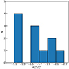 |
Fig. 1. Spectral index distribution of the study sample of 11 radio halos, estimated within a region centered on the halo and with radius 1re. |
First, the starting sample of 20 radio halos has been significantly reduced to a point where the statistics, although still relevant, are too poor to derive any conclusive results. With the currently available data, there is no way to improve our analysis without including systems previously excluded due to uncertain spectral index measurements. However, doing so would introduce different types of uncertainties into our results. In the immediate future, LoLSS DR2 will, however, enable an increase in the number of detectable radio halos. Botteon et al. (2022) find a total of 80 galaxy clusters hosting radio halos in the DR2 of LoTSS. When combining it with LoLSS, it is likely that we will still be forced to exclude a number of systems because of the same issues that impacted this work (low resolution, poor complex source subtraction, etc.). If we assume that a similar fraction (around 50%) of clusters is lost, 40 radio halos will still constitute a significantly large sample, and the results will be considerably more robust. High-resolution observations to be conducted using LOFAR International Stations (IS) and LOFAR2.0 in the coming years will significantly enhance the accuracy of compact source subtraction.
Finally, it is worth noting that a potential tendency is detected for less massive systems in our sample to host halos with steeper spectra, while massive clusters seem to exhibit flatter halos. While this is a crucial prediction of turbulent models, the statistics are too poor to allow for a deeper analysis. Thus, we reserve this discussion for future work, where we will exploit the full DR2 of LoLSS to significantly increase the sample of halos. This is essential since, if confirmed, this would be robust proof that radio halos with very steep spectra are common in radio surveys at low frequencies. The results would clearly support the currently prevalent theoretical picture, which assumes that relativistic electrons in the ICM originate from reacceleration mechanisms activated by cluster merger-driven turbulence, rather than from hadronic processes. Finally, it would conclusively prove that a fraction of the kinetic energy associated with the motions of the matter on large scales is channelled into electromagnetic fluctuations in the plasma and on nonthermal components.
4. Conclusions
In this paper, we have combined data from currently available observations of the two LOFAR surveys, LoTSS and LoLSS, to derive integrated spectral indices for a sample of radio halos. We have discussed our results, including the potential sources of errors and limitations and their impact on formation models of halos. Our results can be summarized as follows:
-
We have followed up with LoLSS a sample of 20 radio halos that were first observed with LoTSS. All of these sources are also detected at 54 MHz. After compact-source subtraction, we excluded nine halos because of leftover AGN or compact emission, resulting from the relatively low resolution of LoLSS, which does not always allow for the accurate subtraction of spurious sources.
-
We measured the halo spectral index between 54 and 144 MHz for all of the remaining 11 radio halos. We find that seven of them (∼64%) have an ultra-steep spectrum (α < −1.5). This is in line with theoretical expectations based on turbulent reacceleration models, which predict a high fraction of ultra-steep spectrum halos at low frequency.
-
We observe a tentative trend indicating that more massive clusters tend to host flatter radio halos. However, due to the currently limited statistical data, we defer a detailed discussion of this observation to future work that will utilize a much larger sample.
-
We have discussed the limitations of our study. The current status of LoLSS and its relatively low-resolution result in low statistics, which cannot be used to conclusively determine the origin of radio halos. LoLSS DR2 will significantly increase the sample, as did LoTSS, whose DR2 contains around 80 new radio halos. Combined with the increased resolution provided by LOFAR international stations, it will finally elucidate the role of turbulent reacceleration in the origin of radio halos in galaxy clusters.
This comes from the proportionality between break frequency and mass; see e.g., Cassano & Brunetti (2005).
RA: 11h to 16h and Dec: 45° to 62°, Hill et al. (2008).
i.e., radio emission detected but no X-ray observation available, as defined in Botteon et al. (2022).
see Appendix C for more details.
Publicly available at https://github.com/revoltek/LiLF
Acknowledgments
We thank the referee for useful comments. M.G. acknowledges support from the ERC Consolidator Grant BlackHoleWeather (101086804). LOFAR (van Haarlem et al. 2013) is the LOw Frequency ARray designed and constructed by ASTRON. It has observing, data processing, and data storage facilities in several countries, which are owned by various parties (each with their own funding sources), and are collectively operated by the ILT foundation under a joint scientific policy. The ILT resources have benefitted from the following recent major funding sources: CNRS-INSU, Observatoire de Paris and Université d’Orléans, France; BMBF, MIWF-NRW, MPG, Germany; Science Foundation Ireland (SFI), Department of Business, Enterprise and Innovation (DBEI), Ireland; NWO, The Netherlands; The Science and Technology Facilities Council, UK; Ministry of Science and Higher Education, Poland; Istituto Nazionale di Astrofisica (INAF), Italy. This research made use of the Dutch national e-infrastructure with support of the SURF Cooperative (e-infra 180169) and the LOFAR e-infra group, and of the LOFAR-IT computing infrastructure supported and operated by INAF, and by the Physics Dept. of Turin University (under the agreement with Consorzio Interuniversitario per la Fisica Spaziale) at the C3S Supercomputing Centre, Italy. The Jülich LOFAR Long Term Archive and the German LOFAR network are both coordinated and operated by the Jülich Supercomputing Centre (JSC), and computing resources on the supercomputer JUWELS at JSC were provided by the Gauss Centre for Supercomputing e.V. (grant CHTB00) through the John von Neumann Institute for Computing (NIC). This research made use of the University of Hertfordshire high-performance computing facility and the LOFAR-UK computing facility located at the University of Hertfordshire and supported by STFC [ST/P000096/1].
References
- Adam, R., Goksu, H., Brown, S., Rudnick, L., & Ferrari, C. 2021, A&A, 648, A60 [NASA ADS] [CrossRef] [EDP Sciences] [Google Scholar]
- Beresnyak, A., Xu, H., Li, H., & Schlickeiser, R. 2013, ApJ, 771, 131 [Google Scholar]
- Bonafede, A., Brüggen, M., van Weeren, R., et al. 2012, MNRAS, 426, 40 [Google Scholar]
- Bonafede, A., Brunetti, G., Rudnick, L., et al. 2022, ApJ, 933, 218 [NASA ADS] [CrossRef] [Google Scholar]
- Botteon, A., Shimwell, T. W., Bonafede, A., et al. 2018, MNRAS, 478, 885 [Google Scholar]
- Botteon, A., van Weeren, R. J., Brunetti, G., et al. 2020, MNRAS, 499, L11 [Google Scholar]
- Botteon, A., Shimwell, T. W., Cassano, R., et al. 2022, A&A, 660, A78 [NASA ADS] [CrossRef] [EDP Sciences] [Google Scholar]
- Boxelaar, J. M., van Weeren, R. J., & Botteon, A. 2021, Adv. Astron. Space Phys., 11, 100464 [Google Scholar]
- Brüggen, M., Bykov, A., Ryu, D., & Röttgering, H. 2012, Space Sci. Rev., 166, 187 [Google Scholar]
- Brunetti, G., & Jones, T. W. 2014, Int. J. Mod. Phys. D, 23, 1430007 [Google Scholar]
- Brunetti, G., Giacintucci, S., Cassano, R., et al. 2008, Nature, 455, 944 [Google Scholar]
- Brunetti, G., & Lazarian, A. 2007, MNRAS, 378, 245 [Google Scholar]
- Brunetti, G., & Lazarian, A. 2011, MNRAS, 410, 127 [Google Scholar]
- Brunetti, G., Setti, G., Feretti, L., & Giovannini, G. 2001, MNRAS, 320, 365 [Google Scholar]
- Brunetti, G., Zimmer, S., & Zandanel, F. 2017, MNRAS, 472, 1506 [Google Scholar]
- Bruno, L., Rajpurohit, K., Brunetti, G., et al. 2021, A&A, 650, A44 [NASA ADS] [CrossRef] [EDP Sciences] [Google Scholar]
- Bruno, L., Brunetti, G., Botteon, A., et al. 2023, A&A, 672, A41 [NASA ADS] [CrossRef] [EDP Sciences] [Google Scholar]
- Buote, D. A. 2001, ApJ, 553, L15 [Google Scholar]
- Cassano, R., & Brunetti, G. 2005, MNRAS, 357, 1313 [Google Scholar]
- Cassano, R., Brunetti, G., & Setti, G. 2006, MNRAS, 369, 1577 [Google Scholar]
- Cassano, R., Brunetti, G., Röttgering, H. J. A., & Brüggen, M. 2010a, A&A, 509, A68 [NASA ADS] [CrossRef] [EDP Sciences] [Google Scholar]
- Cassano, R., Ettori, S., Giacintucci, S., et al. 2010b, ApJ, 721, L82 [Google Scholar]
- Cassano, R., Cuciti, V., Brunetti, G., et al. 2023, A&A, 672, A43 [NASA ADS] [CrossRef] [EDP Sciences] [Google Scholar]
- Cuciti, V., Cassano, R., Brunetti, G., et al. 2021, A&A, 647, A51 [EDP Sciences] [Google Scholar]
- Cuciti, V., de Gasperin, F., Brüggen, M., et al. 2022, Nature, 609, 911 [NASA ADS] [CrossRef] [Google Scholar]
- de Gasperin, F., Williams, W. L., Best, P., et al. 2021, A&A, 648, A104 [NASA ADS] [CrossRef] [EDP Sciences] [Google Scholar]
- de Gasperin, F., Edler, H. W., Williams, W. L., et al. 2023, A&A, 673, A165 [NASA ADS] [CrossRef] [EDP Sciences] [Google Scholar]
- Di Gennaro, G., van Weeren, R. J., Cassano, R., et al. 2021, A&A, 654, A166 [NASA ADS] [CrossRef] [EDP Sciences] [Google Scholar]
- Dolag, K., & Enßlin, T. A. 2000, A&A, 362, 151 [NASA ADS] [Google Scholar]
- Dolag, K., Vazza, F., Brunetti, G., & Tormen, G. 2005, MNRAS, 364, 753 [NASA ADS] [CrossRef] [Google Scholar]
- Donnert, J., & Brunetti, G. 2014, Comput. Astrophys. Cosmol., 1, 5 [Google Scholar]
- Edler, H. W., de Gasperin, F., Brunetti, G., et al. 2022, A&A, 666, A3 [NASA ADS] [CrossRef] [EDP Sciences] [Google Scholar]
- Enßlin, T. A., & Pfrommer, C. 2011, A&A, 527, A99 [NASA ADS] [CrossRef] [EDP Sciences] [Google Scholar]
- Giovannini, G., Tordi, M., & Feretti, L. 1999, New A, 4, 141 [Google Scholar]
- Hill, G. J., Gebhardt, K., Komatsu, E., et al. 2008, ASP Conf. Ser., 399, 115 [Google Scholar]
- Hoeft, M., Dumba, C., Drabent, A., et al. 2021, A&A, 654, A68 [NASA ADS] [CrossRef] [EDP Sciences] [Google Scholar]
- Jaffe, W. J. 1977, ApJ, 212, 1 [NASA ADS] [CrossRef] [Google Scholar]
- Miniati, F. 2015, ApJ, 800, 60 [Google Scholar]
- Nishiwaki, K., Asano, K., & Murase, K. 2021, ApJ, 922, 190 [Google Scholar]
- Offringa, A. R., McKinley, B., Hurley-Walker, N., et al. 2014, MNRAS, 444, 606 [Google Scholar]
- Osinga, E., van Weeren, R. J., Boxelaar, J. M., et al. 2021, A&A, 648, A11 [NASA ADS] [CrossRef] [EDP Sciences] [Google Scholar]
- Pasini, T., Edler, H. W., Brüggen, M., et al. 2022, A&A, 663, A105 [NASA ADS] [CrossRef] [EDP Sciences] [Google Scholar]
- Petrosian, V. 2001, ApJ, 557, 560 [Google Scholar]
- Pfrommer, C., Enßlin, T. A., & Springel, V. 2008, MNRAS, 385, 1211 [Google Scholar]
- Pinzke, A., Oh, S. P., & Pfrommer, C. 2017, MNRAS, 464, 4495 [NASA ADS] [CrossRef] [Google Scholar]
- Planck Collaboration XXVII. 2016, A&A, 594, A27 [NASA ADS] [CrossRef] [EDP Sciences] [Google Scholar]
- Shimwell, T. W., Hardcastle, M. J., Tasse, C., et al. 2022, A&A, 659, A1 [NASA ADS] [CrossRef] [EDP Sciences] [Google Scholar]
- Shimwell, T. W., Röttgering, H. J. A., Best, P. N., et al. 2017, A&A, 598, A104 [NASA ADS] [CrossRef] [EDP Sciences] [Google Scholar]
- Shimwell, T. W., Tasse, C., Hardcastle, M. J., et al. 2019, A&A, 622, A1 [NASA ADS] [CrossRef] [EDP Sciences] [Google Scholar]
- Tasse, C., Shimwell, T., Hardcastle, M. J., et al. 2021, A&A, 648, A1 [EDP Sciences] [Google Scholar]
- van Diepen, G., Dijkema, T. J., & Offringa, A. 2018, Astrophysics Source Code Library [record ascl:1804.003] [Google Scholar]
- van Haarlem, M. P., Wise, M. W., Gunst, A. W., et al. 2013, A&A, 556, A2 [NASA ADS] [CrossRef] [EDP Sciences] [Google Scholar]
- van Weeren, R. J., de Gasperin, F., Akamatsu, H., Brüggen, M., & Feretti, L. 2019, Space Sci. Rev., 215, 16 [NASA ADS] [CrossRef] [Google Scholar]
- van Weeren, R. J., Shimwell, T. W., Botteon, A., et al. 2021, A&A, 651, A115 [NASA ADS] [CrossRef] [EDP Sciences] [Google Scholar]
- Wilber, A., Brüggen, M., Bonafede, A., et al. 2018, MNRAS, 473, 3536 [Google Scholar]
- Willson, M. A. G. 1970, MNRAS, 151, 1 [Google Scholar]
- Zhang, X., Simionescu, A., Gastaldello, F., et al. 2023, A&A, 672, A42 [NASA ADS] [CrossRef] [EDP Sciences] [Google Scholar]
Appendix A: Data calibration
A.1. LBA observations and calibration procedure
Our clusters were observed as part of the LoLSS survey. LoLSS is performed by observing different pointings so that the northern sky at Dec. > 24° is covered with a sensitivity that is close to uniform (see de Gasperin et al. 2021 and de Gasperin et al. 2023 for more detail). Each pointing is independently calibrated using the automated Pipeline for LOFAR LBA (PiLL6). Since all the details are thoroughly discussed in de Gasperin et al. (2021) and de Gasperin et al. (2023), here we only summarize the main steps. Phase and bandpass solutions are derived through the default pre-processing pipeline (DP3, van Diepen et al. 2018) from calibrators that are simultaneously observed with the targets (making use of the multi-beam capability of LOFAR) and transferred to the target field. Faraday rotation, second-order beam errors, and direction-averaged ionospheric delays are then corrected through direction-independent calibration. To correct for direction-dependent errors, all sources are subtracted from the visibilities, and then only the brightest source is re-added (DD calibrator). Calibration solutions are derived from this source through self-calibration in DP3, then subtracted again the DD calibrator more accurately. This process is performed on every sufficiently bright source in the field of view (FoV). The FoV is then divided into facets depending on the positions of all DD sources, calibrating each facet using the solutions of the corresponding DD source. This process is performed through DDFacet (Tasse et al. 2021).
A.2. Extraction and imaging
Each cluster of our sample is covered by one or more survey pointings, which have been calibrated following the standard procedure described above. However, survey images are often affected by issues such as calibration artefacts, smearing (i.e., elongation or blurring of sources) and reduction in dynamic range. These effects occur due to beam errors and ionospheric disturbances, which can be relevant, especially in the case of wide-field images. To improve the image fidelity and dynamic range, we post-process LoLSS data by exploiting a strategy that has already been applied successfully to both 144 MHz observations (van Weeren et al. 2021; Botteon et al. 2022) and 54 MHz observations (e.g., Edler et al. 2022; Cuciti et al. 2022; Pasini et al. 2022). The corresponding workflow is summarized in van Weeren et al. (2021) for 144 MHz data, while we already described our 54 MHz implementation in detail in Pasini et al. (2022). Here we summarize the main steps, which involve an algorithm that has been suitably improved to deal with all current and future LoLSS observations. A region was chosen around the target source in each pointing with beam sensitivity at the target position above 30%. The choice is based on the flux density within this region, which typically has an extent of 15′−20′. All sources outside this extraction region were subtracted, shifting the phase center to the region’s center and averaging all data in time and frequency. Pointings with higher beam sensitivity contribute more to the final combined dataset. Self-calibration was then performed through WSClean (Offringa et al. 2014) and DP3. The accuracy of the flux density scale was compared to LoLSS to check for correctness. The extraction pipeline is included in the Library for Low Frequency (LiLF) package7.
For each target, we produced images at nominal and high resolution, setting Briggs 0 and Briggs -0.6, respectively. We also produced a number of images at low resolution. This was done by setting Briggs -0.3, but tapering visibilities at 30″ and 90″ and to an angular scale corresponding to 50 and 100 kpc at the cluster redshift. In addition, we subtracted compact sources using the following procedure to highlight the diffuse emission better. First, we produced a high-resolution image by setting Briggs -1 and by cutting visibilities below a certain threshold so that everything with the largest linear size (LLS) below 250 kpc gets removed. Therefore, the angular size of the threshold depends on the cluster redshift. We also tested different values, including 350 and 400 kpc, since extended AGN emission (e.g., remnant plasma from past AGN outbursts) likely constitutes the dominant contaminating factor, especially at 54 MHz, when studying diffuse emission. We find that 250 kpc works best for our purposes since it removes the vast majority of AGN emission and leaves diffuse emission intact. The clean components of this high-resolution image that constitute our model were then subtracted from the overall visibilities, leaving only the diffuse emission. We separately produced multiple low-resolution images for these source-subtracted datasets by applying the same tapering discussed above. The typical rms noise is ∼1.5, ∼2.5, and ∼4 mJy beam−1 for nominal resolution, 30″-, and 90″-tapered images, respectively, while tapering visibilities at 50 and 100 kpc usually leads to 1.5 and 1.7 mJy beam−1. Images of the whole sample at both 54 and 144 MHz can be found in Appendix E.
A.3. HBA observations
We exploited the 144 MHz LoTSS observations of our clusters discussed in van Weeren et al. (2021) to estimate the synchrotron spectral index. In particular, we used the same data that was previously extracted and calibrated in Botteon et al. (2022)8. All targets have undergone a similar procedure to what was described above for 54 MHz, including a consistent, compact source subtraction. We refer the reader to van Weeren et al. (2021) and Botteon et al. (2022) for further details.
A.4. X-ray observations
Since radio halos are known to be spatially and physically correlated (Cassano et al. 2010b) with thermal emission from the ICM, we used the same X-ray observations exploited in Botteon et al. (2022) and Zhang et al. (2023) to check the presence of halos at 54 MHz. These are typically archival Chandra or XMM-Newton observations processed with CIAO 4.11 using CalDB v4.8.2 and SAS v16.1.0 following the standard data reduction procedure for the two instruments. We refer to van Weeren et al. (2021) for further calibration details and to Botteon et al. (2022) for the combination with 144 MHz observations.
Appendix B: Initial sample
Table B.1 provides a complete table of the initial sample of PSZ galaxy clusters analyzed in this work.
Properties of the initial sample of PSZ galaxy clusters
Appendix C: Flux density and spectral index measurement
To calculate the spectral indices of these 11 halos, we measured their flux density at 54 and 144 MHz. This was done for each system at the highest resolution at which the combination of image quality, source subtraction, and halo visibility was best. To measure the halo flux density, recent studies (e.g., Osinga et al. 2021; Botteon et al. 2022; Bruno et al. 2023) have exploited the Halo-FDCA algorithm (Boxelaar et al. 2021), which fits the surface brightness radial profile of radio halos with an exponential function. However, the low S/N of most radio halos at 54 MHz does not allow a reliable fit with this procedure. Furthermore, the algorithm is currently not able to simultaneously fit the surface brightness at the two frequencies (see Botteon et al. 2022 for a discussion of the algorithm limitations). This restriction impacts our analysis since performing independent fits at the two frequencies would likely lead us to sample (slightly) different areas of diffuse emission, which would translate into an erroneous spectral index value.
Hence, the calculation of the halo flux density at each frequency is done from circular regions centered on the peak of the halo as detected at 144 MHz in Botteon et al. (2022)9, with a radius corresponding to one e-folding radius (re) as estimated at 144 MHz. This is motivated by the fact that re, which describes the size of the radio halo through an exponential profile I(r)∝e−r/re, is defined as the radius at which the halo surface brightness goes down by a factor of 1/e (and thus is roughly one-third of the emission peak). Therefore, it yields a constant fraction Sre ∼ 30% of the total flux density (e.g., Bruno et al. 2023; Cassano et al. 2023). Typically, 3re is used as a reference, which recovers ∼80% of the total flux density. However, we decided to use 1re to exclude any contamination by spurious sources as much as possible. In some of our systems, using 3re would have implied making wide use of masks, which we tried to avoid to provide a consistent, easily reproducible measurement. Even though we might miss halo flux in the outskirts, it should still provide accurate estimates of the integrated spectral index. Currently, only a few known cases of radio halos show gradients in the synchrotron spectrum steepness moving from the halo center toward the periphery. One of these is the halo hosted in Coma, which is the closest known to date (Brunetti et al. 2001; Bonafede et al. 2022). Nevertheless, we expect the integrated spectral index to be barely affected by any gradient, as it is weighted by the flux density.
Uncertainties on the flux density, S, were then derived using

where f = 0.1 for 144 MHz data and f = 0.06 for 54 MHz data is the absolute flux-scale uncertainty (Shimwell et al. 2019, 2022; de Gasperin et al. 2023), Nbeams the number of beams covering the halo (within 1 re), σrms the image noise, and σsub the uncertainty due to compact source subtraction. The latter is given by
where the sum is taken over all the i sources that were subtracted within the region in which the flux density is estimated.
Residual images were carefully inspected to check for the presence of non-deconvolved emission, which could lead to overestimating the flux density. For all our systems, the flux density within the same region (i.e., a circle with radius = 1re) as measured from residual images was consistent with 0, as expected.
In addition, as an independent check, we also calculated the spectral index by measuring the flux density of each halo at the two frequencies within the 3σ contours derived at 144 MHz. With this method, we might mistakenly include spurious emission that was not completely subtracted by our procedure, but for the majority of the sample, we should still be able to get a good spectral index estimate. With this alternative measurement, our aim is to confirm that using 1re did not yield any bias due, for example, to the relatively small dimensions of the region. Finally, we checked the literature for the few systems for which a spectral index (within the same or a different frequency interval) had already been measured (Botteon et al. 2020; Di Gennaro et al. 2021; Hoeft et al. 2021; Pasini et al. 2022). We find consistent values for the spectral index with all three methods, the only exception being PSZ2G099.86+58.45. In this system, Di Gennaro et al. (2021) reports an overall integrated spectral index of  (measured on the whole halo extent). With our data, we find instead α = −1.67 ± 0.26 between 54 and 144 MHz (within 1re). The discrepancy is most likely due to the combination of a relatively high redshift (z = 0.616), the complex morphology of the source, and a large number of radio AGN located within the halo (see also Fig. A.4 of Di Gennaro et al. (2021)), which all make the subtraction of compact sources significantly harder, especially at 54 MHz where the S/N is lower and the image beam larger. It is also worth noting that Di Gennaro et al. (2021) reports regions with a significantly steeper spectral index (α ∼ −1.6) in the central part of the halo. Although deeper observations would be beneficial in shedding more light on this issue, we still chose to include the system in our sample so as not to introduce a selection effect.
Finally, the spectral index and associated error were estimated by using
where S1 and S2 are the flux densities at frequencies ν1 and ν2, respectively, while σ is the corresponding error.
Appendix D: Selection bias
In this section, we discuss the possibility that the detection of a significant population of USSRH in Fig. 1 might be driven by selection effects that originate from the different sensitivity of LoTSS and LoLSS at their respective frequency. First of all, a straightforward calculation (see also de Gasperin et al. 2023) shows that, if we take into account the reported sensitivity of the two surveys (∼0.1 and ∼1 mJy beam−1 at 144 and 54 MHz, respectively), and we rescale them to the same beam, the spectral index between them is ∼-0.5. This means that sources on the edge of LoTSS sensitivity might not be detected in LoLSS if their spectrum is flatter than this value since their emission at 54 MHz would fall below its sensitivity limit. On the other hand, we should detect all sources with a spectrum steeper than -0.5, including all radio halos.
We also compared the radio power of our halos as a function of the redshift with the sensitivity curves of LoTSS and LoLSS. First we used Eq. 2 from (Cassano et al. 2023) to derive the minimum luminosity detectable at 54 MHz by LoLSS by assuming re = 150 kpc10 at a resolution of 100 kpc (converted into arcseconds at the cluster redshift), which is the typical resolution of the images that we have used to detect radio halos. We assumed a conservative rms noise of 3 mJy/beam, which is the highest noise we find among the images of our halos at that resolution. We did the same for LoTSS, converting the 144 MHz luminosity to 54 MHz by assuming different spectral indices: -1, -1.5, and -2. Finally, we sampled the PSZ2 selection effect, similarly to what was done in (Cassano et al. 2023). We estimated the 150 MHz radio power corresponding to the 50% PSZ2 completeness curve (M, z) in Fig. 1 of (Cassano et al. 2023), using the radio power-cluster mass correlation found for LoTSS-DR2 radio halos (see Eq. 1 of (Cassano et al. 2023)). We then converted the 150 MHz radio power to 54 MHz by assuming a spectral index α = −1.5. The result is shown in Fig. D.1.
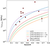 |
Fig. D.1. Radio power at 54 MHz of radio halos vs. redshift (red circles). The purple curve represents the 50% PSZ2 completeness line converted to 54 MHz radio power following the power-mass correlation of (Cassano et al. 2023) and assuming α = −1.5. The blue curve is the minimum luminosity detectable at 54 MHz by LOFAR following Eq. 2 of (Cassano et al. 2023), estimated assuming re= 150 kpc and a resolution of 100 kpc. The red, green, and yellow curves report instead the minimum luminosity detectable at 144 MHz by LOFAR under the same assumptions, converted to 54 MHz assuming α = −2, −1.5, and −1, respectively. |
The plot clearly shows that, within the redshift range of our clusters (0.18 < z< 0.7), the detection of radio halos is not dominated by the sensitivity of either LoTSS or LoLSS, as the vast majority of our systems lie above or are consistent with their minimum luminosity curves. This is also supported by the fact that all our radio halos detected in LoTSS are also observed in LoLSS. The distribution of our clusters in the radio power-redshift plane of Fig. D.1 is determined by the PSZ2 completeness curve, which dominates over the sensitivity of the two surveys. One system (PSZ2G086.93+53.18) lies well below the sensitivity curves. However, the corresponding images are characterized by a lower rms noise than the sensitivity curve (∼3 mJy/beam), and it is the only halo that we detected by tapering visibilities to 90″. We can thus conclude that our results are not substantially driven by selection effects that could prevent the detection of radio halos with different spectral properties, such as the LOFAR sensitivity at the two frequencies.
Appendix E: Images
In this section, we show high- and source-subtracted low-resolution images at 54 and 144 MHz of our sample of radio halos. For each target, the low-resolution images are at the resolution from which the halo flux density was estimated. Images of the whole initial sample of clusters, as well as X-ray maps, can be found at https://lofar-surveys.org/planck_dr2.html.
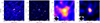 |
Fig. E.1. From left to right: 54 MHz briggs, 144 MHz briggs, 54 MHz low-resolution, and 144 MHz low-resolution images of PSZ2G086.93+53.18. Low-resolution images were produced by tapering visibilities at 90″. Their rms noise is ∼5 and ∼1 mJy beam−1 at 54 and 144 MHz, respectively. The yellow circle denotes 1 re. |
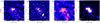 |
Fig. E.2. From left to right: 54 MHz briggs, 144 MHz briggs, 54 MHz low-resolution, and 144 MHz low-resolution images of PSZ2G096.83+52.49. Low-resolution images were produced by tapering visibilities at an angular scale corresponding to 100 kpc at the cluster redshift. Their rms noise is ∼4 and ∼0.15 mJy beam−1 at 54 and 144 MHz, respectively. The yellow circle denotes 1 re. |
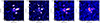 |
Fig. E.3. From left to right: 54 MHz briggs, 144 MHz briggs, 54 MHz low-resolution, and 144 MHz low-resolution images of PSZ2G099.86+58.45. Low-resolution images were produced by tapering visibilities at an angular scale corresponding to 50 kpc at the cluster redshift. Their rms noise is ∼1.7 and ∼0.1 mJy beam−1 at 54 and 144 MHz, respectively. The yellow circle denotes 1 re. |
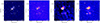 |
Fig. E.4. From left to right: 54 MHz briggs, 144 MHz briggs, 54 MHz low-resolution, and 144 MHz low-resolution images of PSZ2G107.10+65.32. Low-resolution images were produced by tapering visibilities at an angular scale corresponding to 100 kpc at the cluster redshift. Their rms noise is ∼2.5 and ∼0.18 mJy beam−1 at 54 and 144 MHz, respectively. The yellow circles denote 1 re for both halos. |
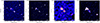 |
Fig. E.5. From left to right: 54 MHz briggs, 144 MHz briggs, 54 MHz low-resolution, and 144 MHz low-resolution images of PSZ2G111.75+70.37. Low-resolution images were produced by tapering visibilities at an angular scale corresponding to 100 kpc at the cluster redshift. Their rms noise is ∼4.4 and ∼0.22 mJy beam−1 at 54 and 144 MHz, respectively. The yellow circle denotes 1 re. |
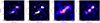 |
Fig. E.6. From left to right: 54 MHz briggs, 144 MHz briggs, 54 MHz low-resolution, and 144 MHz low-resolution images of PSZ2G114.31+64.89. Low-resolution images were produced by tapering visibilities at an angular scale corresponding to 50 kpc at the cluster redshift. Their rms noise is ∼2.4 and ∼0.1 mJy beam−1 at 54 and 144 MHz, respectively. The yellow circle denotes 1 re. |
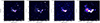 |
Fig. E.7. From left to right: 54 MHz briggs, 144 MHz briggs, 54 MHz low-resolution, and 144 MHz low-resolution images of PSZ2G133.60+69.04. Low-resolution images were produced by tapering visibilities at an angular scale corresponding to 50 kpc at the cluster redshift. Their rms noise is ∼1.5 and ∼0.12 mJy beam−1 at 54 and 144 MHz, respectively. The yellow circle denotes 1 re. |
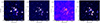 |
Fig. E.8. From left to right: 54 MHz briggs, 144 MHz briggs, 54 MHz low-resolution, and 144 MHz low-resolution images of PSZ2G135.17+65.43. Low-resolution images were produced by tapering visibilities at an angular scale corresponding to 50 kpc at the cluster redshift. Their rms noise is ∼1.5 and ∼0.11 mJy beam−1 at 54 and 144 MHz, respectively. The yellow circle denotes 1 re. |
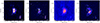 |
Fig. E.9. From left to right: 54 MHz briggs, 144 MHz briggs, 54 MHz low-resolution, and 144 MHz low-resolution images of PSZ2G139.18+56.37. Low-resolution images were produced by tapering visibilities at an angular scale corresponding to 50 kpc at the cluster redshift. Their rms noise is ∼2.3 and ∼0.09 mJy beam−1 at 54 and 144 MHz, respectively. The yellow circle denotes 1 re. |
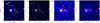 |
Fig. E.10. From left to right: 54 MHz briggs, 144 MHz briggs, 54 MHz low-resolution, and 144 MHz low-resolution images of PSZ2G143.26+65.24. Low-resolution images were produced by tapering visibilities at an angular scale corresponding to 100 kpc at the cluster redshift. Their rms noise is ∼1.8 and ∼0.17 mJy beam−1 at 54 and 144 MHz, respectively. The yellow circle denotes 1 re. |
All Tables
All Figures
|
Fig. 1. Spectral index distribution of the study sample of 11 radio halos, estimated within a region centered on the halo and with radius 1re. |
| In the text | |
|
Fig. D.1. Radio power at 54 MHz of radio halos vs. redshift (red circles). The purple curve represents the 50% PSZ2 completeness line converted to 54 MHz radio power following the power-mass correlation of (Cassano et al. 2023) and assuming α = −1.5. The blue curve is the minimum luminosity detectable at 54 MHz by LOFAR following Eq. 2 of (Cassano et al. 2023), estimated assuming re= 150 kpc and a resolution of 100 kpc. The red, green, and yellow curves report instead the minimum luminosity detectable at 144 MHz by LOFAR under the same assumptions, converted to 54 MHz assuming α = −2, −1.5, and −1, respectively. |
| In the text | |
|
Fig. E.1. From left to right: 54 MHz briggs, 144 MHz briggs, 54 MHz low-resolution, and 144 MHz low-resolution images of PSZ2G086.93+53.18. Low-resolution images were produced by tapering visibilities at 90″. Their rms noise is ∼5 and ∼1 mJy beam−1 at 54 and 144 MHz, respectively. The yellow circle denotes 1 re. |
| In the text | |
|
Fig. E.2. From left to right: 54 MHz briggs, 144 MHz briggs, 54 MHz low-resolution, and 144 MHz low-resolution images of PSZ2G096.83+52.49. Low-resolution images were produced by tapering visibilities at an angular scale corresponding to 100 kpc at the cluster redshift. Their rms noise is ∼4 and ∼0.15 mJy beam−1 at 54 and 144 MHz, respectively. The yellow circle denotes 1 re. |
| In the text | |
|
Fig. E.3. From left to right: 54 MHz briggs, 144 MHz briggs, 54 MHz low-resolution, and 144 MHz low-resolution images of PSZ2G099.86+58.45. Low-resolution images were produced by tapering visibilities at an angular scale corresponding to 50 kpc at the cluster redshift. Their rms noise is ∼1.7 and ∼0.1 mJy beam−1 at 54 and 144 MHz, respectively. The yellow circle denotes 1 re. |
| In the text | |
|
Fig. E.4. From left to right: 54 MHz briggs, 144 MHz briggs, 54 MHz low-resolution, and 144 MHz low-resolution images of PSZ2G107.10+65.32. Low-resolution images were produced by tapering visibilities at an angular scale corresponding to 100 kpc at the cluster redshift. Their rms noise is ∼2.5 and ∼0.18 mJy beam−1 at 54 and 144 MHz, respectively. The yellow circles denote 1 re for both halos. |
| In the text | |
|
Fig. E.5. From left to right: 54 MHz briggs, 144 MHz briggs, 54 MHz low-resolution, and 144 MHz low-resolution images of PSZ2G111.75+70.37. Low-resolution images were produced by tapering visibilities at an angular scale corresponding to 100 kpc at the cluster redshift. Their rms noise is ∼4.4 and ∼0.22 mJy beam−1 at 54 and 144 MHz, respectively. The yellow circle denotes 1 re. |
| In the text | |
|
Fig. E.6. From left to right: 54 MHz briggs, 144 MHz briggs, 54 MHz low-resolution, and 144 MHz low-resolution images of PSZ2G114.31+64.89. Low-resolution images were produced by tapering visibilities at an angular scale corresponding to 50 kpc at the cluster redshift. Their rms noise is ∼2.4 and ∼0.1 mJy beam−1 at 54 and 144 MHz, respectively. The yellow circle denotes 1 re. |
| In the text | |
|
Fig. E.7. From left to right: 54 MHz briggs, 144 MHz briggs, 54 MHz low-resolution, and 144 MHz low-resolution images of PSZ2G133.60+69.04. Low-resolution images were produced by tapering visibilities at an angular scale corresponding to 50 kpc at the cluster redshift. Their rms noise is ∼1.5 and ∼0.12 mJy beam−1 at 54 and 144 MHz, respectively. The yellow circle denotes 1 re. |
| In the text | |
|
Fig. E.8. From left to right: 54 MHz briggs, 144 MHz briggs, 54 MHz low-resolution, and 144 MHz low-resolution images of PSZ2G135.17+65.43. Low-resolution images were produced by tapering visibilities at an angular scale corresponding to 50 kpc at the cluster redshift. Their rms noise is ∼1.5 and ∼0.11 mJy beam−1 at 54 and 144 MHz, respectively. The yellow circle denotes 1 re. |
| In the text | |
|
Fig. E.9. From left to right: 54 MHz briggs, 144 MHz briggs, 54 MHz low-resolution, and 144 MHz low-resolution images of PSZ2G139.18+56.37. Low-resolution images were produced by tapering visibilities at an angular scale corresponding to 50 kpc at the cluster redshift. Their rms noise is ∼2.3 and ∼0.09 mJy beam−1 at 54 and 144 MHz, respectively. The yellow circle denotes 1 re. |
| In the text | |
|
Fig. E.10. From left to right: 54 MHz briggs, 144 MHz briggs, 54 MHz low-resolution, and 144 MHz low-resolution images of PSZ2G143.26+65.24. Low-resolution images were produced by tapering visibilities at an angular scale corresponding to 100 kpc at the cluster redshift. Their rms noise is ∼1.8 and ∼0.17 mJy beam−1 at 54 and 144 MHz, respectively. The yellow circle denotes 1 re. |
| In the text | |
Current usage metrics show cumulative count of Article Views (full-text article views including HTML views, PDF and ePub downloads, according to the available data) and Abstracts Views on Vision4Press platform.
Data correspond to usage on the plateform after 2015. The current usage metrics is available 48-96 hours after online publication and is updated daily on week days.
Initial download of the metrics may take a while.