| Issue |
A&A
Volume 688, August 2024
|
|
|---|---|---|
| Article Number | A136 | |
| Number of page(s) | 13 | |
| Section | Interstellar and circumstellar matter | |
| DOI | https://doi.org/10.1051/0004-6361/202348237 | |
| Published online | 09 August 2024 | |
Weighing protoplanetary discs with kinematics: Physical model, method, and benchmark
1
Univ Lyon, Univ Lyon1, Ens de Lyon, CNRS, Centre de Recherche Astrophysique de Lyon UMR5574,
69230,
Saint-Genis-Laval,
France
e-mail: benedetta.veronesi@ens-lyon.fr
2
Dipartimento di Fisica, Università degli Studi di Milano,
Via Celoria 16,
20133
Milano,
Italy
3
Institute of Astronomy, University of Cambridge,
Madingley Rd,
CB30HA,
Cambridge,
UK
4
Center for Simulational Physics, The University of Georgia,
Athens,
GA
30602,
USA
5
Dipartimento di Fisica e Astronomia “Augusto Righi”
Viale Berti Pichat 6/2,
Bologna,
Italy
6
INAF, Osservatorio Astrofisico di Arcetri,
Largo E. Fermi 5,
50125
Firenze,
Italy
Received:
11
October
2023
Accepted:
22
May
2024
Context. The mass of protoplanetary discs determines the amount of material available for planet formation, the level of coupling between gas and dust, and possibly also sets gravitational instabilities. Measuring the mass of a disc is challenging, as it is not possible to directly detect H2, and CO-based estimates remain poorly constrained.
Aims. An alternative method has recently been proposed that does not rely on tracer-to-H2 ratios. It allows dynamical measurement of the disc mass together with the star mass and the disc critical radius by looking at deviations from Keplerian rotation induced by the self-gravity of the disc. So far, this method has been used to weigh three protoplanetary discs: Elias 2-27, IM Lup, and GM Aurigae.
Methods. We provide a numerical benchmark of the above method. To this end, we simulated isothermal self-gravitating discs with a range of masses from 0.01 to 0.2 M⊙ with the PHANTOM code and post-processed them with radiative transfer (MCFOST) to obtain synthetic observations.
Results. We find that dynamical weighing allows us to retrieve the expected disc masses as long as the disc-to-star mass ratio is larger than Md/M* = 0.05. We estimate an uncertainty for the disc mass measurement of ~25%.
Key words: methods: analytical / methods: numerical / planets and satellites: formation / protoplanetary disks
© The Authors 2024
 Open Access article, published by EDP Sciences, under the terms of the Creative Commons Attribution License (https://creativecommons.org/licenses/by/4.0), which permits unrestricted use, distribution, and reproduction in any medium, provided the original work is properly cited.
This article is published in open access under the Subscribe to Open model. Subscribe to A&A to support open access publication.
1 Introduction
A fundamental but still poorly constrained property of protoplanetary discs is their mass. This parameter is of paramount importance because it affects the planet formation process in many different ways. First of all, it determines the amount of material available for the formation of planets (Manara et al. 2018; Mulders et al. 2021), and, once formed, it can also influence their migration efficiency (e.g. Nelson 2018). Furthermore, it controls the interactions between gas and dust particles through drag, strongly influencing the dynamics of the dust, and therefore also its radial drift and growth (e.g. Birnstiel et al. 2010a,b; Laibe 2014; Gonzalez et al. 2017; Franceschi et al. 2022). The mass of the protopanetary disc can also affect the ionisation rate and thus the magnetic activity (e.g. Lesur et al. 2022). Finally, if the disc-to-star mass ratio is sufficiently high (i.e. q = Mdisc/M* ≳ 0.07–0.1, Kratter & Lodato 2016), the disc self-gravity (SG) affects the morphology and the stability of the system. This may potentially lead to the development of gravitational instability (GI) in the form of a spiral structure (Jeans 1902; Lin & Shu 1964; Paczynski 1978; Binney & Tremaine 1987; Lin & Pringle 1987; Bertin & Lin 1996; Kratter & Lodato 2016), which several authors claim to have observed (e.g. see the case of Elias 2-27, Pérez et al. 2016; Huang et al. 2018; Paneque-Carreño et al. 2021). However, weighing protoplanetary discs is challenging. Indeed, the main disc gaseous component, molecular hydrogen (H2), emits faintly in cold environments, thus making its direct detection extremely difficult. Consequently, one must rely on other gas-mass tracers. A first approach consists in measuring fluxes of alternative gaseous tracers such as CO isotopologues (e.g. Miotello et al. 2017), with 12CO being the most abundant. Then, by assuming a model-dependent conversion factor from CO isotopologues to H2, one can estimate the total mass. Another viable tracer is dust: the gas mass can be estimated by measuring the dust mass from millimetre flux assuming the disc is optically thin and setting a value for the gas-to-dust ratio (e.g. 100 as in the ISM; Draine 2003). However, all these methods rely on conversion factors – which lack accurate constraints – and on the assumption that the observed dust is optically thin (for a more comprehensive review, see Miotello et al. 2023). Another recently investigated tracer is hydrogen deuteride (HD; e.g. Bergin et al. 2013; Trapman et al. 2017). When the disc vertical structure is known, a more reliable estimate of the disc mass can be obtained using HD, which tends to yield higher values compared to other tracers (Trapman et al. 2017). A sufficiently large sample of measurements to test the strength of this method is still missing due to the absence of plans for a far-infrared observatory with the capability to observe HD. Recently, Trapman et al. (2022) investigated the possibility of using a combination of N2H+ and C18O to determine the CO-to-H2 ratio (Öberg et al. 2023), which nevertheless still depends on the assumed disc structure and N2 abundance. Lastly, a handful of additional approaches have been proposed in an attempt to provide a better characterisation of this disc property. For example, by looking at multi-wavelength observations and comparing substructures to get an estimation of the Stokes number, and thus of the total disc mass or local surface density (Powell et al. 2019; Veronesi et al. 2019). Also, by investigating the morphology of a kinematic feature linked to GI, known as GI-wiggle (Hall et al. 2020; Longarini et al. 2021), Terry et al. (2022) recently found an approximately linear relationship between the amplitude of this wiggle and the disc-to-star mass ratio, thus obtaining an estimate of the mass of gravitationally unstable discs.
An alternative approach to tracers and dust-to-H2 conversion has recently been proposed (Veronesi et al. 2021; Lodato et al. 2023), which consists in dynamically measuring the mass of the disc. Indeed, when the disc is massive enough compared to the star, the gravity of the disc contributes considerably to the azimuthal gas velocity, making it super-Keplerian. In particular, the azimuthally averaged rotation curve is expected to transition from an inner Keplerian profile to an outer flatter one, indicative of the disc contribution. If high-resolution kinematic data are available, the observed rotation curve can be fitted, allowing a dynamical mass estimate to be obtained. This method has been widely used in galaxies (e.g. Barbieri et al. 2005) and has also been applied to AGN discs (e.g. Lodato & Bertin 2003). It is also worth noting that it does not require precision on previous stellar mass measurements, because it simultaneously fits M* and the disc mass, Md, from the rotation curve. To date, in the context of protoplanetary discs, the method has been applied to three systems, Elias 2-27 (Veronesi et al. 2021), IM Lup, and GM Aur (Lodato et al. 2023), providing a disc-to-star mass ratio (~0.1–0.4) for the first two that is consistent with a scenario where the detected spirals are induced by GI.
This method of dynamical measurement, which is efficient for massive discs, relies on a simple model for the structure and the dynamics of the disc. As such, it is important to determine the range of disc-to-stellar mass within which it can provide sufficiently accurate results. In this study, we provide a benchmark of the method by performing a set of smoothedparticle hydrodynamics (SPH) and radiative transfer simulations (PHANTOM+MCFOST, Price et al. 2018; Pinte et al. 2009), taking into account the gravity of the disc.
This article is organised as follows: in Sec. 2 we describe the physical model use for the gas. In Sec. 3, we present and benchmark our set of numerical simulations. In Sect. 4, we detail the analysis workflow and present our results. In Sec. 5, we present our analysis of the uncertainties. In Sect. 6, we discuss these uncertainties and highlight some possible limitations and future outlooks. We finally draw our conclusions in Sec. 7.
2 Physical model
We consider a smooth axisymmetric circular disc, and we neglect the effect of the magnetic field and dust feedback. Indeed, the former brings only a small correction to the turbulence and magnetic pressure, while the latter may only significantly modify the effect of the pressure gradient of the gas for high dust-to-gas ratios, which is assumed not to be the case for the systems studied here. We also do not consider discs with embedded planets. Low-mass planets would introduce a negligible correction of the order of ∝Mp/M*. Massive planets would create gaps and modify the gas surface densities, but this is beyond the scope of this first exploration. Within these assumptions, the azimuthal velocity vϕ of a gas particle at a cylindrical distance R and height z from a central object of mass M* is related to the gas pressure P and the gravitational potential of the disc Φd according to
![$\[v_\phi^2=\frac{\mathcal{G} M_{\star} R^2}{\left(R^2+z^2\right)^{3 / 2}}+\frac{R}{\rho} \frac{\partial P(R, z)}{\partial R}+R \frac{\partial \Phi_{\mathrm{d}}}{\partial R}.\]$](/articles/aa/full_html/2024/08/aa48237-23/aa48237-23-eq1.png) (1)
(1)
The three contributions of the right hand-side of Eq. (1) correspond to the gravity of the central star, the radial pressure gradient, and the self-gravity of the disc. We assume that the surface density of the gas follows a self-similar profile set by turbulent viscosity (Lynden-Bell & Pringle 1974):
![$\[\Sigma(R)=\frac{M_{\mathrm{d}}(2-\gamma)}{2 \pi R_{\mathrm{c}}^2}\left(\frac{R}{R_{\mathrm{c}}}\right)^{-\gamma} \exp \left[-\left(\frac{R}{R_{\mathrm{c}}}\right)^{2-\gamma}\right],\]$](/articles/aa/full_html/2024/08/aa48237-23/aa48237-23-eq2.png) (2)
(2)
where Rc is the tapering radius, Md the disc mass, and γ = 1 is the power-law index. Although this profile is commonly used for non-self-gravitating discs, it can also be chosen in the self-gravitating case since the Keplerian shear is not affected by the disc SG. We also assume the disc to be vertically isothermal with the density profile given by
![$\[\rho(R, z)=\rho_0(R) \exp \left[-\frac{R^2}{H^2}\left(1-\frac{1}{\sqrt{1+z^2 / R^2}}\right)\right] \text {, }\]$](/articles/aa/full_html/2024/08/aa48237-23/aa48237-23-eq3.png) (3)
(3)
and the temperature profile to be a power law with the radius
![$\[T(R)=T_{100}\left(\frac{R}{100 \mathrm{~au}}\right)^{-q},\]$](/articles/aa/full_html/2024/08/aa48237-23/aa48237-23-eq4.png) (4)
(4)
where H is the disc thickness, ρ0 is the density at the mid-plane, and T100 is a normalisation factor at 100 au. We stress that the discs considered are not only vertically but also locally isothermal (see Sec. 3.1).
Following, for example, Lodato et al. (2023), the rotation profile is
![$\[\begin{aligned}v_\phi^2= & v_{\mathrm{K}}^2\left\{1-\left[\gamma^{\prime}+(2-\gamma)\left(\frac{R}{R_{\mathrm{c}}}\right)^{2-\gamma}\right]\left(\frac{H}{R}\right)^2\right. \\& \left.-q\left(1-\frac{1}{\sqrt{1+(z / R)^2}}\right)\right\}+v_d^2,\end{aligned}\]$](/articles/aa/full_html/2024/08/aa48237-23/aa48237-23-eq5.png) (5)
(5)
![$\[\gamma^{\prime}=\gamma+3 / 2+q / 2, v_{\mathrm{K}}^2=\mathcal{G} M_{\star} / R\]$](/articles/aa/full_html/2024/08/aa48237-23/aa48237-23-eq6.png)
![$\[\begin{aligned}v_{\mathrm{d}}^2= & \mathcal{G} \int_0^{\infty}\left[K(k)-\frac{1}{4}\left(\frac{k^2}{1-k^2}\right)\right. \\& \left.\times\left(\frac{r}{R}-\frac{R}{r}+\frac{z^2}{R r}\right) E(k)\right] \sqrt{\frac{r}{R}} k \Sigma(r) \mathrm{d} r,\end{aligned}\]$](/articles/aa/full_html/2024/08/aa48237-23/aa48237-23-eq7.png)
where K(k) and E(k) are complete elliptic integrals and k2 = 4Rr/[(R + r)2 + z2] (Binney & Tremaine 1987; Bertin & Lodato 1999). Here the boundaries of the integral are chosen to correspond to the inner and outer radius of the disc. The terms have been rearranged in four contributions: (1) a purely circular Keplerian term, ![$\[v_{\mathrm{K}} \equiv \sqrt{\mathcal{G} M_{\star} / R}\]$](/articles/aa/full_html/2024/08/aa48237-23/aa48237-23-eq8.png) ; (2) a term related to the radial pressure gradient in the midplane, which gives a sub-Keplerian contribution; (3) another sub-Keplerian term originating from the pressure gradient and the stellar contribution in the vertical direction; and finally (4) the self-contribution of the disc (see Eq. (6)). To be able to compare some of these contributions, we present some orders of magnitude. The correction introduced by the vertical dependence of the stellar potential is ~(z/R)2 and is therefore of the same order as the correction due to the pressure gradient, and therefore should not be neglected (we derived the disc mass of Elias 2-27 with the updated model, obtaining a result that is consistent with Veronesi et al. 2021; see Appendix A). In Appendix B, these equations are provided in a dimensionless form for order-of-magnitude estimates.
; (2) a term related to the radial pressure gradient in the midplane, which gives a sub-Keplerian contribution; (3) another sub-Keplerian term originating from the pressure gradient and the stellar contribution in the vertical direction; and finally (4) the self-contribution of the disc (see Eq. (6)). To be able to compare some of these contributions, we present some orders of magnitude. The correction introduced by the vertical dependence of the stellar potential is ~(z/R)2 and is therefore of the same order as the correction due to the pressure gradient, and therefore should not be neglected (we derived the disc mass of Elias 2-27 with the updated model, obtaining a result that is consistent with Veronesi et al. 2021; see Appendix A). In Appendix B, these equations are provided in a dimensionless form for order-of-magnitude estimates.
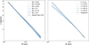 |
Fig. 1 Rotation curves extracted from SPH simulations. Left: rotation curves in the midplane of the disc extracted from the SPH simulations with H/R100au = 0.075 after 20 orbits at the outer disc radius, for different disc-to-star mass ratios (solid lines). The black dash-dotted line shows the rotation curve of the model given by Eq. (5), including the pressure gradient term with zero disc mass. Except for profiles obtained with a disc-to-star mass ratio of 0.01, the rotation curves are distinct from a model without the disc self-gravity. Right: same as left panel but with Mdisc = 0.1 M⊙, with rotation curves extracted for different heights (blue solid lines), and compared to the one obtained in the midplane (z = 0, black dashed-dot line). |
3 Numerical simulations
3.1 Hydrodynamical simulations
We performed a suite of 3D SPH simulations of gaseous protoplanetary discs using the code PHANTOM (Price et al. 2018). The system consists of a central star of mass M* = 1 M⊙ surrounded by a gas disc with mass Mdisc = [0.01, 0.025, 0.05, 0.1, 0.15, 0.2] M⊙. These simulations can be rescaled in terms of disc-to-star mass ratio (see the derivation in Appendix B). The disc extends from Rin = 10 au to Rout = 300 au, and is simulated with 106 SPH particles. The initial profile of surface density is a relaxed exponential tapered power law of Eq. (2), with Rc = 100 au and γ = 1. Simulations include the disc self-gravity as described in Price et al. (2018), adopting a locally isothermal equation of state ![$\[P=c_{\mathrm{s}}^2 \rho_{\mathrm{g}}\]$](/articles/aa/full_html/2024/08/aa48237-23/aa48237-23-eq9.png) with q = 0.5 for the power-law index of the temperature radial profile (see Eq. (4)). As a consequence of the absence of cooling, the morphology of the discs will be smooth and axisymmetric, without spiral density waves due to gravitational instability. This is consistent with the fact that, to date, most of the observed discs are axisymmetric (with or without substructures; Ohashi et al. 2023). Effects of self-gravity can be important even if the disc does not host spirals. The choice of the index for radial profile of temperature would remain valid even if we were to take into account dust in the hydrodynamical modelling, because variations in the temperature q-index are not expected to significantly impact the evolution of dust (Pinte & Laibe 2014).
with q = 0.5 for the power-law index of the temperature radial profile (see Eq. (4)). As a consequence of the absence of cooling, the morphology of the discs will be smooth and axisymmetric, without spiral density waves due to gravitational instability. This is consistent with the fact that, to date, most of the observed discs are axisymmetric (with or without substructures; Ohashi et al. 2023). Effects of self-gravity can be important even if the disc does not host spirals. The choice of the index for radial profile of temperature would remain valid even if we were to take into account dust in the hydrodynamical modelling, because variations in the temperature q-index are not expected to significantly impact the evolution of dust (Pinte & Laibe 2014).
The disc is vertically extended by initially setting up a disc aspect ratio of (H/R)c = 0.075 with a Gaussian profile for the volume density (see Eq. (3)), ensuring nearly vertical hydrostatic equilibrium. These locally isothermal simulations do not require an extra cooling term. As such, we model the angular momentum transport throughout the disc using the SPH shock to capture viscosity (Price et al. 2018, see Sect. 2.6) with αAV ≃ 0.19, which results in a Shakura & Sunyaev (1973) viscous parameter of αss ≈ 0.005. The parameters used are given in Appendix C.
3.2 Preliminary test: Hydrodynamical rotation curves
As a first benchmark, we first extracted the rotation curves directly from the hydrodynamical simulations after having relaxed the disc to centrifugal equilibrium (t ~ 20Ωout, where Ωout is the orbital period of the disc outer radius). The rotation curves are obtained by interpolating azimuthal velocities of the SPH particles along the desired coordinates (R, z), and then azimuthally averaging the results. This step provides an uncertainty for the rotational velocity that is estimated as a standard deviation. Figure 1 shows the rotation curves obtained by this procedure. The left panel shows the rotation profiles obtained in the midplane (R, z = 0), with disc masses ranging from 0.01 to 0.2 (blue lines). As a reference, the black line provides the rotation curve of the model given by Eq. (5)), including the pressure gradient term, but setting the mass of the disc to zero. As expected, the contribution of the disc self-gravity increases with the disc-to-star mass ratio. The right panel shows the rotation curves of the simulation with Mdisc = 0.1 at different heights ranging from z = 0 to z = 50 au. As expected from the model, the difference in azimuthal velocity between different heights decreases with radius.
To benchmark the validity of the formulation given by Eq. (5), we fit the extracted rotation curves with the code dysc1, which implements the model described in Sec. 2. The results are shown in Table 1. The fitting procedure relies on a Markov Chain Monte Carlo using the Python package EMCEE (Foreman-Mackey et al. 2013). We used a Gaussian likelihood with flat priors. The code simultaneously fits both the masses of the star and the disc, as well as the truncation radius Rc, similarly to the procedure described in Lodato et al. (2023). After this step, we recovered the mass of the disc with an uncertainty of ~5–12% (see Table 1) for disc-to-star mass ratios ranging between 0.025 and 0.2. In these cases, discs are sufficiently massive for the self-gravity to have a measurable contribution. For a disc-to-star mass ratio of 0.01, the disc mass cannot be extracted accurately even from the numerical simulations.
3.3 Radiative transfer and synthetic observations
We then computed the thermal structure and synthetic observations of our numerical discs by performing 3D radiative transfer simulations with the code MCFOST (Pinte et al. 2006, 2009). We used a Voronoi tessellation, where each MCFOST cell corresponds to a gas SPH particle. The goal is to generate mock 12CO and 13CO isotopologue channel maps, from which we can extract disc rotation curves.
The main inputs for the radiative transfer modelling are the source of luminosity, the gas density profile extracted from the simulations, and models for dust opacities and densities. Self-gravitating isothermal discs do not present any kind of substructure and the underlying dust density profile can therefore be assumed to be smooth. We do not account for an eventual dust drift, since Stokes numbers are expected to be small in these discs, and we consider sufficiently short disc evolutions. The dust contribution to the gravitational potential of the disc is also negligible. As such, we adopt a constant dust-to-gas ratio of ~10−2, which corresponds to a standard averaged ISM (Draine 2003).
The thermal structure of the disc is computed with the following assumptions. At first, emission is at local thermal equilibrium and Tgas = Tdust. Dust is treated as a mixture of silicates (70%) and carbon (30%) (Draine & Lee 1984), and the optical properties are calculated using Mie theory for spheres (Andrews et al. 2009). Opacities are computed following the procedure described in the DIANA model (Woitke et al. 2016; Min et al. 2016). We assume an ISM-like grain size distribution (dn/da ∝ a−3.5), with amin = 0.01 μm and amax = 1 mm. The disc is heated passively, that is, the source of radiation is only the central star, which is assumed to radiate isotropically with a Kurucz spectrum at 4000 K. The expected channel maps are computed via ray tracing, using 107 photon packets to sample the radiation field. The disc inclination with respect to the line of sight is i = 30°, and the system is simulated to be located at 140 pc, which corresponds to a typical protostellar disc in a star-forming region such as Taurus. For 12CO and 13CO, we consider the J = 2–1 transition and assume abundances of 10−4 and 1.4 × 10⁻⁶ respectively. MCFOST simulations are post-processed with PYMCFOST2 by simulating a velocity resolution of 0.1 km s−1. We then spatially convolve the channels with a Gaussian beam of 0.1 arcsec, similarly to the value of the MAPS survey (Öberg et al. 2021). We finally introduce Gaussian noise with an RMS of 5mJy beam−1.
Figure 2 shows an example of the channel maps obtained for a simulation with a disc mass of 0.1 M⊙. The 12CO channels appear more radially extended compared to the 13CO channels. The 13CO channels are also less patchy, because the τ = 1 region is located closer to the midplane, a region with higher resolution. As a result, the 13CO disc rotation curves will be less noisy than the curves extracted from the 12CO channels (see Fig. 5). We note that while this is the case for simulations, in real observations we do not expect 13CO rotation curves to be less noisy than the 12CO. Indeed, 13CO is much less abundant than 12CO, and at the same sensitivity, the signal-to-noise ratio (S/N) in 13CO should be lower than that for 12CO.
4 Method and results
4.1 Workflow description
From the cubes of synthetic data, we first determined the height of the emitting layer with DISKSURF (Teague et al. 2021). The emitting layer is defined as the region from which the emission we observe originates. Isotopologues have specific optical depth and column density, and as such, the emitting layer can be located farther from or closer to the midplane of the disc. Having a precise estimate of the height of the emitting layer is crucial in order to correctly deproject azimuthal velocities and compute the model of Eq. (5) at the correct height.
We then used EDDY (Teague 2019) to extract the rotation curves. Two methods have been developed to retrieve the observed velocity (specifically to fit the line centroids): one quadratic and the other Gaussian. The aim of the former is to fit a quadratic curve to the brightest pixel on either side of the maximum of the pixel. The fit depends on the velocity sampling, and is sensitive to the channel correlation. On the other hand, with the latter method, which finds the line centre by fitting a Gaussian profile to it, the selected velocity range may affect the result in cases with skewed profiles.
To perform our analysis, we chose the quadratic method; we briefly discuss this choice in Sec. 4.3 (for an extended discussion of the methods, see e.g. Lodato et al. 2023 and Teague & Foreman-Mackey 2018). Finally, we fit the rotation curves with the model of Eq. (5) using the code DYSC (see Sec. 2).
4.2 Retrieving the height of the emitting layer
We first used the code DISKSURF (Teague et al. 2021) to extract the height of the emitting layer zn (ri) of the ith radial bin for the nth channel. DISKSURF implements the method presented in Pinte et al. (2018). Briefly, this is a geometrical method that allows the user to trace the emission maxima of each velocity channel and reconstruct the position of the CO layers. For each bin, we determined the heights ![$\[z_{16}^n\left(r_i\right), z_{50}^n\left(r_i\right) \text {, and } z_{84}^n\left(r_i\right)\]$](/articles/aa/full_html/2024/08/aa48237-23/aa48237-23-eq10.png) , which correspond to the 16th, 50th, and 84th percentiles of the distribution, respectively. We then used the tapered power law,
, which correspond to the 16th, 50th, and 84th percentiles of the distribution, respectively. We then used the tapered power law,
![$\[z(R)=z_0[\operatorname{arcsec}]\left(\frac{R}{1 \operatorname{arcsec}}\right)^\psi \exp \left[-\left(\frac{R}{R_t}\right)^{q_t}\right],\]$](/articles/aa/full_html/2024/08/aa48237-23/aa48237-23-eq11.png) (7)
(7)
to continuously parametrise the emitting surfaces z16 (r), zem (r) = z50 (r), and z84 (r). The parameters obtained were used to retrieve the height of the molecular emission surface zem (r) as well as to estimate the uncertainties associated with the procedure.
Table 2 presents the results obtained for zem(r), which we subsequently used as a reference surface in the following analysis. As an example, Fig. 3 shows the emission surface (grey markers) obtained with DISKSURF for the 12CO datacube from a mock observation generated by a simulation with Mdisc = 0.1 M⊙. The three lines are the fits of the data points, namely zem = z50 (solid line), z16 (dotted line), and z84 (dashed line). The scatter between the three fitted surfaces is important with this procedure: it is therefore crucial to refer to this dispersion when analysing uncertainties on the rotation curve.
As expected, we also find that there is a clear trend between the height of the emitting layer and the disc mass: more massive discs have a higher emitting layer, because their surface density is higher and they are optically thicker. Also, the height of the 13CO is lower with respect to the 12CO because of its reduced abundance, tracing a region closer to the midplane. This is shown in more detail in Figs. D.1 and D.2.
Finally, for consistency, we decided not to include the simulation with Md/M* = 0.2 in our analysis at this stage. Indeed, in this case, the 12CO emission is poorly reproduced because the SPH resolution at the emitting surface is not sufficient (see Sec. 6.1 for a resolution analysis).
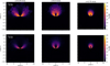 |
Fig. 2 Example of channel maps obtained with MCFOST for the 12CO (top row) and 13CO (bottom row) isotopologues, for a simulation with disc mass of Md = 0.1 M⊙. Different velocity channels are displayed, from 0.25 to 0.75 km s−1 (going from left to right). The chosen Gaussian beam used to convolve the image matches the value of the MAPS survey (0.1″), and is shown with a grey circle in the left bottom corner of each channel map. The velocity resolution is chosen to be 0.1 km s−1 (as in the MAPS survey). |
12CO and 13CO fit results for the parameters relevant to the disc emitting layer (z0, ψ, Rt, qt) obtained with DISKSURF from the 50th percentiles of the particle vertical distribution.
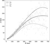 |
Fig. 3 Example (12CO, Mdisc = 0.1 M⊙) of one of the emitting layers derived with DISKSURF (grey dots) and then fitted with an exponentially tapered power law (solid line). We also show the 16th (dotted line) and the 84th (dashed line) percentiles, which we take into account to compute the rotation curve errors. |
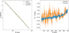 |
Fig. 4 Differences between rotation curves obtained with the Gaussian and quadratic methods. Left panel: comparison between the rotation curves from the model (black line, Eq. (5) with a disc mass of Md = 0.1 M⊙), the Gaussian method (blue line), and the quadratic method (orange line). We observe that the Gaussian curve is systematically shifted with respect to the model. Right panel: difference between the extracted rotation curve (Gaussian method in blue, quadratic method in orange) and the model vϕ from Eq. (5). |
4.3 Extracting the rotation curve
We extract the azimuthal velocity with EDDY (Teague 2019) using the harmonic oscillator method, following Teague et al. (2018a,b). Further details of the extraction methods can be found in Sect. 3.3.1 of Lodato et al. (2023).
For each emitting layer, that is, z16, zem = z50, and z84, we computed three rotation curves, v16, v50, and v84. We then assumed the azimuthal velocity of the system to be v;em = v50, with an uncertainty σv estimated to be
![$\[\sigma_v=\sqrt{\left|v_{84}-v_{16}\right|^2+\sigma_{\text {eddy }}^2} \text {, }\]$](/articles/aa/full_html/2024/08/aa48237-23/aa48237-23-eq12.png) (8)
(8)
where σeddy is the numerical error obtained with EDDY. This procedure refines the approach of Lodato et al. (2023) by including uncertainties related to the estimate of the height of the emitting layer.
As we fixed the inclination of the disc to i = 30°, we used the quadratic method to extract the rotation curve; this method fits only the peak of emission, which is less sensitive to the lower surface. Indeed, using the Gaussian method instead provides the following bias: the emission coming from the lower surface systematically shifts the position of the line centroids, resulting in a systematic error for the velocity estimate. Figure 4 shows a comparison between the quadratic and the Gaussian methods. Interestingly, despite being smoother, the curve obtained with the Gaussian method underestimates the velocity in the inner disc and overestimates it in the outer disc. This happens because the method tries to fit a double-peaked spectrum with a single Gaussian. We note that in this work we tested both methods, and despite both being biased, we chose the quadratic method (although noisier) because the Gaussian one presents an overall larger systematic shift of the velocity caused by the lower surface. Moreover, with the quadratic method we already manage to recover the correct disc and star masses. For completeness, we also tested our workflow using a rotation curve retrieved with a double Gaussian fit. However, the double-Gaussian method fails to retrieve the correct velocity in the outer region of the disc (R > 300 au), where the S/N is too low (it fits the noise but not the signal; see Appendix E).
Figure 5 shows the rotation curves obtained with the quadratic method for both CO isotopologues following the procedure described above (12CO in the left panel, 13CO in the right panel). We compare these with the analytical rotation curve obtained assuming a disc of zero mass (black dash-dotted line). As expected, the rotation curve derived with this approximation fits only the disc with the lower mass (Md = 0.01 M⊙), because this is the only case where the disc contribution can be considered as negligible. We show how we confirmed this in Sec. 4.5.
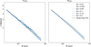 |
Fig. 5 Quadratic rotation curves obtained for all the disc mass simulations (from Mdisc = 0.01 M⊙ to Mdisc = 0.2 M⊙) for the 12CO isotopologue (solid lines in the left panel) and the 13CO isotopologue (dashed lines in the right panel). The black dash-dotted line shows the analytical rotation curve obtained by only considering the star and pressure gradient contribution. |
4.4 Fitting procedure
For every simulation, we obtain two rotation curves: one for 12CO and another for 13CO. These curves are then fitted using the self-gravitating model of Eq. (5). The free parameters are the star and disc mass, and the disc truncation radius. The fits were performed with an MCMC algorithm as implemented in EMCEE (Foreman-Mackey et al. 2013). We chose a simple Gaussian likelihood, and flat priors of [0,5] M⊙ for the star mass3, [50, 300] au for the truncation radius, and [0, 0.5] M⊙ for the disc mass. We chose 250 walkers and 1000 steps (having verified that convergence is reached). We fit the two isotopologues both individually and then simultaneously.
4.5 Fit results
Table 3 shows the values retrieved for the star mass M*, the disc mass Md, and the disc truncation radius Rc for simulations with disc masses ranging within Md = 0.01–0.2 M⊙, and a disc aspect ratio of 0.075. The disc-to-star mass ratio threshold below which the expected value cannot be recovered is 0.05. For reasons related to resolution, we also exclude the simulation with Md = 0.2 M⊙ (see Sec. 4.2). From our procedure, we are able to measure a non-zero value for the disc mass (Mdisc ≥ 0.05 M⊙), which indicates that the model for the rotation curve should include the term from the gravity of the disc.
5 Uncertainties
5.1 Physical parameters
In the treatment of real data, the three principal sources of uncertainty are the height of the emitting layer, the aspect ratio of the disc, and its inclination. Uncertainties on z(r) are estimated with the values of z16 and z84 found previously. To estimate uncertainties associated with H/r and i, we first note that in the fitting procedure of Sec. 4, we enforce the values of H/r and i that were set in the numerical simulation. We therefore estimated uncertainties associated to those parameters by carrying the fit over the same synthetic channel maps while varying H/r and i over a range of values. For H/r, we simply performed new fits over the previously extracted rotation curves. For a setup value of H/R = 0.075, we tested H/R = [0.05, 0.07, 0.08, 0.1]. For inclinations, uncertainty estimates require the extraction of new disc emitting layers, necessitating that we obtain novel rotation curves. For a setup value of i = 30°, we tested i = [27, 29, 31, 33]°. The values of the uncertainties obtained by this procedure are summarised in Table 3. Figure 6 shows these uncertainties for discs whose mass can be accurately recovered by the fitting procedure. This excludes the md0.01 and md0.025 (small masses), and md0.2 (lack of resolution). A key result of this study is that disc masses of self-gravitating discs can be estimated from channel maps with averaged systematic uncertainties of the order of 25%. The three parameters H/r, i, and z make similar contributions as sources of error. No clear trend appears when varying H/r and z. Values that differ from the expected one still provide mass estimates with the same level of uncertainty. On the other hand, precise values of i provide uncertainties of the order of 5–10%, whereas an error of a few degrees provides uncertainties of the order of 20–30%. Hence, our procedure is relatively reliable in its capacity to accurately determine disc masses. For instance, when recovering a disc mass of 0.1 M⊙, the estimated range spans from 0.075 to 0.125. We note that one obtains simultaneously ΔM*/M* ~ 8% for an inclination error of ±3° and ΔRc/Rc ~ 15% for a reasonable disc aspect ratio range of ±0.025 (see Appendix F for a discussion).
5.2 Spatial resolutions
In order to test how the minimum detectable mass is affected by the spatial resolution, we produced new synthetic images by convolving the channel maps previously obtained in Sec. 3.3 with different Gaussian beam sizes [0.2, 0.3]″. We then extracted new rotation curves with the procedure described in Sects. 4.2 and 4.3, and we fit them with the DYSC code (Sec. 4.4). In Fig. 7, we report the results obtained for the disc mass (different markers and lines), showing uncertainties obtained as a function of the spatial resolution of the observations. When Md = 0.05 M⊙, the uncertainty ranges from ~50 to 100%, while for the other two cases, Md = [0.1–0.15] M⊙, it ranges within ~30–40%ο, which is larger compared to the 0.1″ case discussed above (~25%; see Sec. 5.1). This analysis shows that a resolution of 0.1″ is recommended in order to obtain a reliable measurement.
Results for the 12CO, 13CO, and the combined fit procedure.
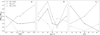 |
Fig. 6 Uncertainties related to the fitting procedure for the disc mass Md. Estimates are given as functions of the aspect ratio of the disc H/R (left column), the disc inclination (middle column), and the disc emitting layer z(R) (right column). Different markers and line styles represent results obtained for simulations with different disc masses. |
6 Discussion
6.1 Numerical resolution
As the height of the emitting layer increases with the disc mass, in the md0.2 simulation, we notice that the emitting layer is higher than the typical height of SPH particles, while this is not true for the case with low disc mass (for an example, see Fig. D.3). Indeed, the number density of SPH particles decreases with z, because most of the disc mass is concentrated in the midplane. This implies that the size of the Voronoi grid cells used in MCFOST is increasing with z, which results in artificially low-resolution 12CO data cubes for the high-disc-mass simulation. To test this, we performed additional hydrodynamical simulations with 2, 4, and 6 × 10⁶ SPH particles. Figure 8 shows that by increasing the number of SPH particles, the uncertainty we obtain for the disc mass decreases until we reach the ‘true’ disc mass value for the 6M particles simulation. The blue dashed line represents the semi-log linear fit of the data points.
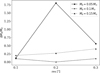 |
Fig. 7 Uncertainties obtained from our fitting procedure for the disc mass ΔMd/Md and for the combined fit procedure with different spatial resolutions [0.1,0.2,0.3]″. Different markers (and lines) represent results obtained for simulations with different disc masses. |
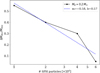 |
Fig. 8 Uncertainties obtained from our fitting procedure for the disc mass ΔMd/Md for the combined fit procedure with different numerical resolutions: [1, 2, 4, 6] × 106 SPH particles. The blue dashed line is the semi-log linear fit of the data points with slope m = −0.58. As expected, accuracy increases with numerical resolution. |
6.2 Limitations and further work
The main assumptions adopted in this study are as follows:
Model: axisymmetric discs, no magnetic field, no planets;
Hydrodynamic simulations: gas only, as the dust-to-gas ratio is assumed to be so low that it does not affect the result. The disc is assumed to be locally and vertically isothermal;
Radiative transfer: Tgas = Tdust (LTE), Mie theory for optical properties, ISM-like grain size distribution, dust-to-gas ratio of ~0.01.
Post-processing of synthetic images: the simulated ALMA images are obtained by convolving with a Gaussian beam and the noise has been added directly to the resulting images. Thus, the filtering of an interferometer and the noise properties of ALMA observations are not fully captured with these simple assumptions. As a test, we also applied the method presented in this work to a simulated ALMA image obtained with CASA, finding no difference in the fitted disc parameters.
Our study is restricted to stable self-gravitating discs, excluding those with peculiar substructures such as GI spirals. It would be important to reproduce the benchmark performed in this study with more general cases; for example, to confirm masses estimated for Elias 2-27, IM Lup, and GM Aur. This study highlights the need to investigate how the extraction of the rotation curve is affected by the presence of non-axisymmetric structures (e.g. by including cooling and allowing the disc to develop GI in the shape of spiral structures). Indeed, non-axisymmetric structures might be important in young objects that are still accreting from the molecular clouds (e.g. streamers). It may also be worth investigating whether or not the presence of an embedded planet or a central binary affects disc mass estimates. Finally, the case of non-isothermal discs is being investigated by Martire et al. (2024).
7 Conclusions
In this study, we benchmarked the determination of disc masses using rotation curves extracted from channel maps as introduced in Veronesi et al. (2021) and Lodato et al. (2023). We generated controlled mock observations from PHANTOM SPH simulations with different disc masses that are post-processed with the MCFOST radiative transfer code. We adopted spatial and spectral resolutions that are the same as those of the MAPS survey (0.1″ and 0.1 km s−1).
We find that for Md/M* ≳ 0.05, we recover the correct disc-to-star mass ratio with a typical accuracy of ~25%, with equal uncertainty contributions from determinations of the aspect ratio and the inclination of the disc, as well as the height of the emitting layer (the truncation radius and the stellar mass are also obtained with uncertainties of ~15% and ~8%, respectively). For lower resolutions (0.2–0.3″), disc masses recovered shift towards larger values (0.1 M⊙ for 0.2″). This constraint should be accounted for when proposing ALMA kinematics observations in order to dynamically measure the disc mass. This method can be used to calibrate existing methods such as those based on flux.
Acknowledgements
The authors want to thank the referee for constructive comments that improved this manuscript. This work has received funding from the ERC CoG project PODCAST No 864965, and from the European Union’s Horizon 2020 research and innovation programme under the Marie Sklodowska-Curie grant agreement no. 823823 (RISE DUSTBUSTERS project). S.F. is funded by the European Union (ERC, UNVEIL, 101076613). Views and opinions expressed are however those of the author(s) only and do not necessarily reflect those of the European Union or the European Research Council. Neither the European Union nor the granting authority can be held responsible for them. We used the EMCEE algorithm Foreman-Mackey et al. (2013), the CORNER package Foreman-Mackey (2016) to produce corner plots, and PYTHON-based MATPLOTLIB package Hunter (2007) for all the other figures. Computational resources were provided by the PSMN (Pôle Scientifique de Modélisation Numérique) of the ENS de Lyon, and the INDACO Platform, a project of High Performance Computing at the Università degli Studi di Milano. The authors thank Pietro Curone, Andrés F. Izquierdo, Sean Andrews, Richard Teague, Giovanni Rosotti and Enrico Ragusa for useful discussions.
Appendix A Elias 2-27 updated fit results
We derived with the updated model the disc mass of Elias 2-27, obtaining a result that is consistent with the findings of Veronesi et al. (2021). In particular, when fitting the west and the east side of the disc simultaneously, and the two isotopologues (13CO and C18O), we obtain a star mass of ~0.40 M⊙ and a disc mass of −0.13 M⊙ (~0.46 M⊙ and ~0.08 M⊙ in Veronesi et al. 2021).
Appendix B Dimensionless model
Equation 5 can be expressed in terms of x = R/Rc and ζ = z/Rc as
![$\[v_\phi^2 / \frac{G M_{\star}}{R_c}=f_1(x, \zeta)+\frac{1}{2 \pi} \frac{M_{\mathrm{d}}}{M_{\star}} f_2(x, \zeta),\]$](/articles/aa/full_html/2024/08/aa48237-23/aa48237-23-eq13.png) (B.1)
(B.1)
![$\[f_1(x, \zeta)=\frac{1}{x}\left\{1-\left[\gamma^{\prime}+(2-\gamma) x^{2-\gamma}\right]\left(\frac{H_{\mathrm{c}}}{R_{\mathrm{c}}}\right)^2 x^{1-q}-q\left(1-\frac{1}{\sqrt{1+\zeta^2}}\right)\right\} \text {, }\]$](/articles/aa/full_html/2024/08/aa48237-23/aa48237-23-eq14.png)
![$\[\begin{array}{r}f_2(x, \zeta)=\int_0^{\infty}\left[K(y)-\frac{1}{4}\left(\frac{y^2}{1-y^2}\right)\left(\frac{u}{x}-\frac{x}{u}+\frac{\zeta^2}{x u}\right) E(y)\right] \\\sqrt{\frac{u}{x}} y \tilde{\Sigma}(u) \mathrm{d} u,\end{array}\]$](/articles/aa/full_html/2024/08/aa48237-23/aa48237-23-eq15.png)
where Hc denotes the scale height at the tapered radius ![$\[R_{\mathrm{c}}, y \equiv\frac{4 u}{(u+x)^2+\zeta^2}, \tilde{\Sigma}\left(r / R_{\mathrm{c}}\right) \equiv \Sigma(r) / \frac{\tilde{M}_{\mathrm{d}}}{2 \pi R_{\mathrm{c}}^2}\]$](/articles/aa/full_html/2024/08/aa48237-23/aa48237-23-eq16.png) denotes the dimensionless surface density, and
denotes the dimensionless surface density, and ![$\[\tilde{M}_{\mathrm{d}} \equiv 2 \pi \int_{R_{\text {in }}}^{R_{\text {out }}} R \Sigma(R) \mathrm{~d} R \simeq M_{\mathrm{d}}\]$](/articles/aa/full_html/2024/08/aa48237-23/aa48237-23-eq17.png) denotes the true mass of the disc. Hence, the azimuthal velocity can be rescaled in terms of the disc-to-star-mass ratio Md/M*.
denotes the true mass of the disc. Hence, the azimuthal velocity can be rescaled in terms of the disc-to-star-mass ratio Md/M*.
Parameters of our SPH simulations.
Appendix C Simulation parameters
The parameters used in the hydrodynamic simulations described in Sect. 3.1 are given in Table B.1.
Appendix D Properties of the emitting layer
Figure D.1 shows the height of emitting layers as a function of the radius for different disc masses. As expected, the emitting layer is higher for large disc masses, because the column density is larger. Fig. D.2 highlights the difference between the height of layers derived for the 12CO (orange line) and 13CO (blue line) isotopologues. 13CO is optically thinner than 12CO and therefore traces a region closer to the midplane; its emitting layer is also lower compared to that of 12CO.
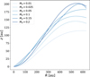 |
Fig. D.1 Emitting layer derived with DISKSURF for different disc masses for the 12CO isotopologue. |
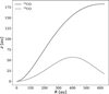 |
Fig. D.2 Comparison between the emitting layer of 12CO (solid line) and 13CO (dashed line) for a disc mass of 0.1 M⊙. |
Fig. D.3 shows a comparison between the emitting layers derived for 0.2 M⊙ (top panel) and 0.025 M⊙ (bottom panel). Emitting layers are plotted with orange solid lines, while the SPH particles particles are represented with cyan markers. The number density of SPH particles decreases with z, as most of the disc mass tends to be concentrated in the midplane. This implies that the size of the Voronoi grid cells increases with z, resulting in an artificially low resolution in the upper layer of the 12CO data cubes. This becomes problematic in the case of the high-disc-mass simulations (e.g. here 0.2 M⊙ for 106 SPH particles), as the disc is optically thicker and the emitting layer is higher with respect to the case of lighter discs.
 |
Fig. D.3 Distribution of SPH particles (cyan dots) and the emitting layer obtained with DISKSURF (orange line) for two simulations, one with high mass (upper panel) and one with low mass (lower panel). |
Appendix E Double Gaussian method
Fig. E.1 shows a comparison between the analytical rotation curve obtained with the self-gravitating model (Eq. 5), and the velocity values obtained with the quadratic and the double Gaussian methods, computed at two different radii. We note that, in the outer region, the value extracted with the double Gaussian method deviates further from the expected value. Moreover, in the outer region the S/N is too low, and the double Gaussian method fits the noise rather than the signal.
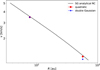 |
Fig. E.1 Comparison among the analytical rotation curve obtained with the self-graviting model (Eq. 5, black solid line), and the velocity obtained with the quadratic (red circle) and the double Gaussian method (blue star), computed at two different radii (70 au and 560 au). |
Appendix F Other uncertainties
Fig. F.1 shows the uncertainties for the mass of the star (top row) and the disc truncation radius (bottom row) as function of the aspect ratio of the disc H/R (left), the disc inclination (centre), and the disc emitting layer z(R) (right). While for the uncertainties for the disc mass (see Fig. 6), the three parameters H/R, i, and z(r) make similar contributions as sources of error, now we can identify two main contributions. For the mass of the star and the disc truncation radius, the principal sources of uncertainty are the inclination of the disc (panel e in Fig. F.1) and its aspect ratio (panel g in Fig. F.1), respectively. Indeed, varying the inclination with respect to the expected value implies that the annulus along which the observed velocity is computed in order to extract the rotation curve is not at a constant radius. Another source of error is related to the deprojection of the rotation curve. This strongly affects the fitted value of the mass of the star. As for the aspect ratio, it mostly influences the truncation radius, as it scales with (H/R)2 (Eq. 5).
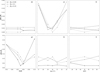 |
Fig. F.1 Uncertainties related to the fitting procedure for the mass of the star M* (top row) and the disc truncation radius Rc (bottom row). Estimates are given as functions of the aspect ratio of the disc H/R (left column), the disc inclination (middle column), and the disc emitting layer z(R) (right column). Different markers and lines styles represent results obtained for simulations with different disc masses. |
References
- Andrews, S. M., Wilner, D. J., Hughes, A. M., Qi, C., & Dullemond, C. P. 2009, ApJ, 700, 1502 [CrossRef] [Google Scholar]
- Barbieri, C. V., Fraternali, F., Oosterloo, T., et al. 2005, A&A, 439, 947 [NASA ADS] [CrossRef] [EDP Sciences] [Google Scholar]
- Bergin, E. A., Cleeves, L. I., Gorti, U., et al. 2013, Nature, 493, 644 [Google Scholar]
- Bertin, G., & Lin, C. C. 1996, Spiral Structure in Galaxies a Density Wave Theory [Google Scholar]
- Bertin, G., & Lodato, G. 1999, A&A, 350, 694 [NASA ADS] [Google Scholar]
- Binney, J., & Tremaine, S. 1987, Galactic Dynamics (Princeton, NJ: Princeton University Press) [Google Scholar]
- Birnstiel, T., Dullemond, C. P., & Brauer, F. 2010a, A&A, 513, A79 [NASA ADS] [CrossRef] [EDP Sciences] [Google Scholar]
- Birnstiel, T., Ricci, L., Trotta, F., et al. 2010b, A&A, 516, A14 [Google Scholar]
- Draine, B. T. 2003, ARA&A, 41, 241 [NASA ADS] [CrossRef] [Google Scholar]
- Draine, B. T., & Lee, H. M. 1984, ApJ, 285, 89 [NASA ADS] [CrossRef] [Google Scholar]
- Foreman-Mackey, D. 2016, J. Open Source Softw., 1, 24 [Google Scholar]
- Foreman-Mackey, D., Hogg, D. W., Lang, D., & Goodman, J. 2013, PASP, 125, 306 [Google Scholar]
- Franceschi, R., Birnstiel, T., Henning, T., et al. 2022, A&A, 657, A74 [NASA ADS] [CrossRef] [EDP Sciences] [Google Scholar]
- Gonzalez, J. F., Laibe, G., & Maddison, S. T. 2017, MNRAS, 467, 1984 [NASA ADS] [Google Scholar]
- Hall, C., Dong, R., Teague, R., et al. 2020, ApJ, 904, 148 [NASA ADS] [CrossRef] [Google Scholar]
- Huang, J., Andrews, S. M., Pérez, L. M., et al. 2018, ApJ, 869, L43 [Google Scholar]
- Hunter, J. D. 2007, Comput. Sci. Eng., 9, 90 [NASA ADS] [CrossRef] [Google Scholar]
- Jeans, J. H. 1902, Philos. Trans. Roy. Soc. Lond. Ser. A, 199, 1 [NASA ADS] [CrossRef] [Google Scholar]
- Kratter, K., & Lodato, G. 2016, ARA&A, 54, 271 [NASA ADS] [CrossRef] [Google Scholar]
- Laibe, G. 2014, MNRAS, 437, 3037 [CrossRef] [Google Scholar]
- Lesur, G., Ercolano, B., Flock, M., et al. 2022, arXiv e-prints [arXiv:2203.09821] [Google Scholar]
- Lin, C. C., & Shu, F. H. 1964, ApJ, 140, 646 [Google Scholar]
- Lin, D. N. C., & Pringle, J. E. 1987, MNRAS, 225, 607 [Google Scholar]
- Lodato, G., & Bertin, G. 2003, A&A, 398, 517 [NASA ADS] [CrossRef] [EDP Sciences] [Google Scholar]
- Lodato, G., Rampinelli, L., Viscardi, E., et al. 2023, MNRAS, 518, 4481 [Google Scholar]
- Longarini, C., Lodato, G., Toci, C., et al. 2021, ApJ, 920, L41 [NASA ADS] [CrossRef] [Google Scholar]
- Lynden-Bell, D., & Pringle, J. E. 1974, MNRAS, 168, 603 [Google Scholar]
- Manara, C. F., Morbidelli, A., & Guillot, T. 2018, A&A, 618, A3 [NASA ADS] [CrossRef] [EDP Sciences] [Google Scholar]
- Martire, P., Longarini, C., Lodato, G., et al. 2024, A&A, 686, A9 [Google Scholar]
- Min, M., Rab, C., Woitke, P., Dominik, C., & Ménard, F. 2016, A&A, 585, A13 [NASA ADS] [CrossRef] [EDP Sciences] [Google Scholar]
- Miotello, A., van Dishoeck, E. F., Williams, J. P., et al. 2017, A&A, 599, A113 [NASA ADS] [CrossRef] [EDP Sciences] [Google Scholar]
- Miotello, A., Kamp, I., Birnstiel, T., Cleeves, L. I., & Kataoka, A. 2023, Protostars and Planets VII, ed. by S. Inutsuka, Y. Aikawa, T. Muto, K. Tomida, & M. Tamura, ASP Conf. Ser., 534, 501 [NASA ADS] [Google Scholar]
- Mulders, G. D., Pascucci, I., Ciesla, F. J., & Fernandes, R. B. 2021, ApJ, 920, 66 [NASA ADS] [CrossRef] [Google Scholar]
- Nelson, R. P. 2018, in Handbook of Exoplanets, eds. H. J. Deeg, & J. A. Belmonte, 139 [Google Scholar]
- Öberg, K. I., Guzmán, V. V., Walsh, C., et al. 2021, ApJS, 257, 1 [CrossRef] [Google Scholar]
- Öberg, K. I., Facchini, S., & Anderson, D. E. 2023, ARA&A, 61, 287 [CrossRef] [Google Scholar]
- Ohashi, N., Tobin, J. J., Jørgensen, J. K., et al. 2023, ApJ, 951, 8 [NASA ADS] [CrossRef] [Google Scholar]
- Paczynski, B. 1978, Acta Astron., 28, 91 [Google Scholar]
- Paneque-Carreño, T., Pérez, L. M., Benisty, M., et al. 2021, ApJ, 914, 88 [CrossRef] [Google Scholar]
- Pérez, L. M., Carpenter, J. M., Andrews, S. M., et al. 2016, Science, 353, 1519 [Google Scholar]
- Pinte, C., & Laibe, G. 2014, A&A, 565, A129 [NASA ADS] [CrossRef] [EDP Sciences] [Google Scholar]
- Pinte, C., Ménard, F., Duchêne, G., & Bastien, P. 2006, A&A, 459, 797 [NASA ADS] [CrossRef] [EDP Sciences] [Google Scholar]
- Pinte, C., Harries, T. J., Min, M., et al. 2009, A&A, 498, 967 [NASA ADS] [CrossRef] [EDP Sciences] [Google Scholar]
- Pinte, C., Ménard, F., Duchêne, G., et al. 2018, A&A, 609, A47 [NASA ADS] [CrossRef] [EDP Sciences] [Google Scholar]
- Powell, D., Murray-Clay, R., Pérez, L. M., Schlichting, H. E., & Rosenthal, M. 2019, ApJ, 878, 116 [NASA ADS] [CrossRef] [Google Scholar]
- Price, D. J., Wurster, J., Tricco, T. S., et al. 2018, PASA, 35, e031 [Google Scholar]
- Shakura, N. I., & Sunyaev, R. A. 1973, A&A, 24, 337 [NASA ADS] [Google Scholar]
- Teague, R. 2019, J. Open Source Softw., 4, 1220 [Google Scholar]
- Teague, R., & Foreman-Mackey, D. 2018, RNAAS, 2, 173 [NASA ADS] [Google Scholar]
- Teague, R., Bae, J., Bergin, E. A., Birnstiel, T., & Foreman-Mackey, D. 2018a, ApJ, 860, L12 [NASA ADS] [CrossRef] [Google Scholar]
- Teague, R., Bae, J., Birnstiel, T., & Bergin, E. A. 2018b, ApJ, 868, 113 [Google Scholar]
- Teague, R., Law, C. J., Huang, J., & Meng, F. 2021, J. Open Source Softw., 6, 3827 [NASA ADS] [CrossRef] [Google Scholar]
- Terry, J. P., Hall, C., Longarini, C., et al. 2022, MNRAS, 510, 1671 [Google Scholar]
- Trapman, L., Miotello, A., Kama, M., van Dishoeck, E. F., & Bruderer, S. 2017, A&A, 605, A69 [NASA ADS] [CrossRef] [EDP Sciences] [Google Scholar]
- Trapman, L., Zhang, K., van’t Hoff, M. L. R., Hogerheijde, M. R., & Bergin, E. A. 2022, ApJ, 926, L2 [NASA ADS] [CrossRef] [Google Scholar]
- Veronesi, B., Lodato, G., Dipierro, G., et al. 2019, MNRAS, 489, 3758 [Google Scholar]
- Veronesi, B., Paneque-Carreño, T., Lodato, G., et al. 2021, ApJ, 914, L27 [NASA ADS] [CrossRef] [Google Scholar]
- Woitke, P., Min, M., Pinte, C., et al. 2016, A&A, 586, A103 [NASA ADS] [CrossRef] [EDP Sciences] [Google Scholar]
All Tables
12CO and 13CO fit results for the parameters relevant to the disc emitting layer (z0, ψ, Rt, qt) obtained with DISKSURF from the 50th percentiles of the particle vertical distribution.
All Figures
|
Fig. 1 Rotation curves extracted from SPH simulations. Left: rotation curves in the midplane of the disc extracted from the SPH simulations with H/R100au = 0.075 after 20 orbits at the outer disc radius, for different disc-to-star mass ratios (solid lines). The black dash-dotted line shows the rotation curve of the model given by Eq. (5), including the pressure gradient term with zero disc mass. Except for profiles obtained with a disc-to-star mass ratio of 0.01, the rotation curves are distinct from a model without the disc self-gravity. Right: same as left panel but with Mdisc = 0.1 M⊙, with rotation curves extracted for different heights (blue solid lines), and compared to the one obtained in the midplane (z = 0, black dashed-dot line). |
| In the text | |
|
Fig. 2 Example of channel maps obtained with MCFOST for the 12CO (top row) and 13CO (bottom row) isotopologues, for a simulation with disc mass of Md = 0.1 M⊙. Different velocity channels are displayed, from 0.25 to 0.75 km s−1 (going from left to right). The chosen Gaussian beam used to convolve the image matches the value of the MAPS survey (0.1″), and is shown with a grey circle in the left bottom corner of each channel map. The velocity resolution is chosen to be 0.1 km s−1 (as in the MAPS survey). |
| In the text | |
|
Fig. 3 Example (12CO, Mdisc = 0.1 M⊙) of one of the emitting layers derived with DISKSURF (grey dots) and then fitted with an exponentially tapered power law (solid line). We also show the 16th (dotted line) and the 84th (dashed line) percentiles, which we take into account to compute the rotation curve errors. |
| In the text | |
|
Fig. 4 Differences between rotation curves obtained with the Gaussian and quadratic methods. Left panel: comparison between the rotation curves from the model (black line, Eq. (5) with a disc mass of Md = 0.1 M⊙), the Gaussian method (blue line), and the quadratic method (orange line). We observe that the Gaussian curve is systematically shifted with respect to the model. Right panel: difference between the extracted rotation curve (Gaussian method in blue, quadratic method in orange) and the model vϕ from Eq. (5). |
| In the text | |
|
Fig. 5 Quadratic rotation curves obtained for all the disc mass simulations (from Mdisc = 0.01 M⊙ to Mdisc = 0.2 M⊙) for the 12CO isotopologue (solid lines in the left panel) and the 13CO isotopologue (dashed lines in the right panel). The black dash-dotted line shows the analytical rotation curve obtained by only considering the star and pressure gradient contribution. |
| In the text | |
|
Fig. 6 Uncertainties related to the fitting procedure for the disc mass Md. Estimates are given as functions of the aspect ratio of the disc H/R (left column), the disc inclination (middle column), and the disc emitting layer z(R) (right column). Different markers and line styles represent results obtained for simulations with different disc masses. |
| In the text | |
|
Fig. 7 Uncertainties obtained from our fitting procedure for the disc mass ΔMd/Md and for the combined fit procedure with different spatial resolutions [0.1,0.2,0.3]″. Different markers (and lines) represent results obtained for simulations with different disc masses. |
| In the text | |
|
Fig. 8 Uncertainties obtained from our fitting procedure for the disc mass ΔMd/Md for the combined fit procedure with different numerical resolutions: [1, 2, 4, 6] × 106 SPH particles. The blue dashed line is the semi-log linear fit of the data points with slope m = −0.58. As expected, accuracy increases with numerical resolution. |
| In the text | |
|
Fig. D.1 Emitting layer derived with DISKSURF for different disc masses for the 12CO isotopologue. |
| In the text | |
|
Fig. D.2 Comparison between the emitting layer of 12CO (solid line) and 13CO (dashed line) for a disc mass of 0.1 M⊙. |
| In the text | |
|
Fig. D.3 Distribution of SPH particles (cyan dots) and the emitting layer obtained with DISKSURF (orange line) for two simulations, one with high mass (upper panel) and one with low mass (lower panel). |
| In the text | |
|
Fig. E.1 Comparison among the analytical rotation curve obtained with the self-graviting model (Eq. 5, black solid line), and the velocity obtained with the quadratic (red circle) and the double Gaussian method (blue star), computed at two different radii (70 au and 560 au). |
| In the text | |
|
Fig. F.1 Uncertainties related to the fitting procedure for the mass of the star M* (top row) and the disc truncation radius Rc (bottom row). Estimates are given as functions of the aspect ratio of the disc H/R (left column), the disc inclination (middle column), and the disc emitting layer z(R) (right column). Different markers and lines styles represent results obtained for simulations with different disc masses. |
| In the text | |
Current usage metrics show cumulative count of Article Views (full-text article views including HTML views, PDF and ePub downloads, according to the available data) and Abstracts Views on Vision4Press platform.
Data correspond to usage on the plateform after 2015. The current usage metrics is available 48-96 hours after online publication and is updated daily on week days.
Initial download of the metrics may take a while.