| Issue |
A&A
Volume 686, June 2024
|
|
|---|---|---|
| Article Number | A210 | |
| Number of page(s) | 20 | |
| Section | Cosmology (including clusters of galaxies) | |
| DOI | https://doi.org/10.1051/0004-6361/202348955 | |
| Published online | 12 June 2024 | |
A proposal to improve the accuracy of cosmological observables and address the Hubble tension problem
1
Institut für Astrophysik, Universitätssternwarte Wien, Fakultät für Geowissenschaften, Geographie und Astronomie, Universität Wien, Türkenschanzstr. 17, 1180 Vienna, Austria
e-mail: horst.foidl@outlook.com, tanja.rindler-daller@univie.ac.at
2
Vienna International School of Earth and Space Sciences, Universität Wien, Josef-Holaubek-Platz 2, 1090 Vienna, Austria
3
Wolfgang Pauli Institut, Oskar-Morgenstern-Platz 1, 1090 Vienna, Austria
Received:
14
December
2023
Accepted:
25
March
2024
Context. Cosmological observational programs often compare their data not only with Λ cold dark matter (ΛCDM), but also with extensions applying dynamical models of dark energy (DE), whose time-dependent equation of state (EoS) parameters w differ from that of a cosmological constant. We found a degeneracy in the customary computational procedure for the expansion history of cosmological models once dynamical models of DE models were applied. This degeneracy, given the Planck-based Hubble constant H0, provides an infinite number of cosmological models reproducing the Planck-measured cosmic microwave background (CMB) spectrum, including the one with a cosmological constant. Moreover, this degeneracy biases the comparison of ΛCDM with dynamical DE extensions.
Aims. We present a complementary computational approach, that breaks this degeneracy in the computation of the expansion history of models with a dynamical DE component: the “fixed early densities (EDs)” approach evolves cosmological models from the early Universe to the present, in contrast to the customary “fixed H0” approach, which evolves cosmological models in reverse order. Although there are no equations to determine these EDs from first principles, we find they are accurately approximated by the ΛCDM model.
Methods. We implemented a refined procedure, applying both approaches, in an amended version of the code CLASS, where we focused on representative dynamical DE models using the Chevallier-Polarski-Linder (CPL) parametrization, studying cases with monotonically increasing and decreasing w over cosmic time.
Results. Our results reveal that a dynamical DE model with a decreasing w of the form w(a) = − 0.9 + 0.1(1 − a) could provide a resolution to the Hubble tension problem. Moreover, we find that combining the fixed EDs approach and the customary fixed H0 approach, while requesting to yield consistent results and being in agreement with observations across cosmic time, can serve as a kind of consistency check for cosmological models with a dynamical model of DE. Finally, we argue that implementing our proposed consistency check for cosmological models within current Markov chain Monte Carlo (MCMC) methods will increase the accuracy of inferred cosmological parameters significantly, in particular for extensions to ΛCDM.
Conclusions. Using our complementary computational scheme, we find characteristic signatures in the late expansion histories of cosmological models, allowing a phenomenological discrimination of DE candidates and a possible resolution to the Hubble tension, by ongoing and future observational programs.
Key words: cosmological parameters / cosmology: observations / cosmology: theory / dark energy
© The Authors 2024
 Open Access article, published by EDP Sciences, under the terms of the Creative Commons Attribution License (https://creativecommons.org/licenses/by/4.0), which permits unrestricted use, distribution, and reproduction in any medium, provided the original work is properly cited.
This article is published in open access under the Subscribe to Open model. Subscribe to A&A to support open access publication.
1. Introduction
The current cosmological standard model of Λ cold dark matter (ΛCDM) is based on many different observations of the Universe on large scales, especially the cosmic microwave background (CMB; for example, readers can refer to the balloon observations of millimetric extragalactic radiation and geophysics (BOOMERanG) experiment by de Bernardis et al. 2000; MacTavish et al. 2006, as well as observations with an increasing accuracy by the space missions Wilkinson Microwave Anisotropy Probe WMAP; Hinshaw et al. 2013 and Planck; Planck Collaboration VI 2020), the large-scale structure of the cosmic web (for example, readers can refer to the Dark Energy Survey DES; Abbott et al. 2022a, the (extended) Baryon Oscillation Spectroscopic Survey eBOSS and BOSS; Alam et al. 2021, Large Synoptic Survey Telescope; LSST Science Collaboration 2009), and measurements of the distance ladder using stellar standard candles (see e.g., Perlmutter et al. 1999; Schmidt et al. 1998; Riess et al. 1998; Perlmutter 2003). However, the model comes with two major conundra, namely the still unknown nature of CDM and the nature of the cosmological constant Λ which, according to measurements, each contribute roughly 25% and 70%, respectively, to the present-day energy density of the Universe. In attempts to better understand and constrain these components, an accurate measurement of the expansion rate, or Hubble parameter, over cosmic time is desired. Over recent years, discrepancies have been solidified between the measurement of this Hubble parameter at low redshifts z, the (local) Hubble constant H0, and the value of the latter if high-z data, notably encoded in the CMB, are extrapolated to the present. This issue goes under the header of the Hubble tension (problem), and seems to be in conflict with basic assumptions of the ΛCDM model. In particular, the question arises as to whether Λ should be replaced by a dark energy (DE) component, whose energy density and equation of state (EoS) can vary with time, in order to fit cosmological observables at various scales. Since the nature of Λ has defied a resolution as yet, despite theoretical efforts over decades, the Hubble tension adds even more urgency to investigate alternatives in the form of various DE models, which can be tested this way, using ever more precise measurements.
A recent review of the Hubble tension problem can be found in Hu & Wang (2023). There are two major approaches to test models of DE as possible answers to the Hubble tension problem. The first approach uses a parametrization ansatz of the EoS parameter of the DE component, such as the Chevallier-Polarski-Linder (CPL) parametrization (discussed shortly, see Eq. (1)), and it fits this model to observational data, determining the parameters of the dynamical model of DE. Alternatively, the EoS parameter of the DE component can be inferred directly from data. Recent studies (e.g., Dainotti et al. 2021, 2022a,b; Bargiacchi et al. 2023a,b; Ó Colgáin et al. 2021; Krishnan et al. 2021) indicate that the evolution of the expansion rate H at low redshift is in conflict with the assumption of a cosmological constant preferring a dynamical model of DE. These results may indicate that the origin of the Hubble tension is likely to be in cosmology and not in local measurement issues (e.g., Krishnan et al. 2021), as observations with an increasing accuracy of H0 in the local Universe seem to confirm the Hubble tension (e.g., Dainotti et al. 2023a; Khalife et al. 2024).
Many cosmological observation campaigns analyze their data, not only in light of testing ΛCDM, but also to examine the possible signature of DE candidates with a time-varying EoS. Examples include DES; readers can refer to the Year 3 (DES-Y3) results in Abbott et al. (2022a), or the CMB measurements by Planck Collaboration VI (2020). These and other campaigns often employ a dynamical model of DE, with a possible time-dependent EoS parameter w = p/ρ, where p and ρ constitute a pressure and energy density, in some averaged sense or fluid approach. A useful representation of choice has been the so-called CPL parametrization by Chevallier & Polarski (2001) and Linder (2003) for the EoS parameter,

which is defined for a ∈ [0, 1], where a is the scale factor1 of the Friedmann-Lemaître-Robertson-Walker (FLRW) model of the isotropic and homogenous background universe, while w0 and wa are parameters that depend upon the specific DE model. However, in using this form in the comparisons with observations, they are merely free parameters. A cosmological constant Λ is recovered as a special case if w0 = −1 and wa = 0, such that wΛ = −1 throughout the cosmic evolution.
The CPL parametrization offers a variation of w such that DE models can be studied, which evolve linearly in a from w ≃ w0 + wa in the early Universe to w0 at the present at a = 1. Now, campaigns such as Abbott et al. (2022a) and Planck Collaboration VI (2020) compute from their data the probability distribution of models in the (w0 − wa)-plane (parameter subspace). They find that the probability of a cosmological constant is within the 1σ area, “fitted” by a multidimensional Monte Carlo integration to their observational data, using the Markov chain Monte Carlo (MCMC) method (see e.g., Carlin & Louis 2008). While a DE component cannot be definitely ruled out, a cosmological constant is in accordance with both the data in Abbott et al. (2022a) and Planck Collaboration VI (2020). Furthermore, it is common practice to include data or constraints derived from previous literature in the analysis of the observed data (e.g., DES-Y3 includes results from CMB observations and low-z data from baryon acoustic oscillations (BAO)).
However, while statistically in agreement with ΛCDM, it appears that various cosmological observations may prefer different CPL models, in the sense that the (mean value of the) parameter wa is found to be either positive or negative, as we will discuss. It remains to be seen, whether these slight statistical preferences for one or the other eventually converge to a common result, or whether differences pertain pointing to physical explanations, such as a changing EoS of DE. The work in this paper relates to this question, as follows.
The process of inferring parameters of cosmological models from observations depends upon the way they are extracted from measurements. In case the cosmological observable can be measured directly, such as H0 in the local universe (e.g., Riess et al. 2022), there is no or only little dependence on a specific cosmological model. High-redshift data (e.g., CMB temperature spectra by Planck Collaboration VI 2020) is analyzed by specifying a cosmological model (e.g., ΛCDM) and by “fitting” the model to the data. Inherent to this procedure is the computation of a cosmological model (ΛCDM or any of its extensions) and the extrapolation of the model parameters to the present (see e.g., Alam et al. 2021). These present-day values then enter the customary computation procedure of FLRW models. This customary computational procedure starts the backward-in-time integration of the equations determining the expansion history at the present, applying a present-day value of the Hubble parameter H0, that is using a specific value of H0. We call it the “fixed H0” approach in the forthcoming. Thus, the initial densities in the early Universe are determined by the considered model and the provided value of H0. We present a complementary approach, that is based on the assumptions that the initial densities of the cosmic components were determined by processes in the very early Universe, evolving even prior to the point in time, where the computation of cosmological models customarily starts. We call this approach the “fixed early densities (EDs)” approach, that is particularly relevant for cosmic components having a time-dependent EoS parameter, as we exemplify below.
Indeed, there are no equations to determine the initial energy densities in the early Universe from first principles. But we use the fact that these early densities can be approximated to high accuracy by the ΛCDM concordance model, given that in the radiation-dominated and then CDM-dominated epochs, any DE component would be very much subdominant, similar to Λ. More precisely, the two approaches can be characterized as follows. The customary fixed H0 approach starts the computation at the present with the provided value of H0 and integrates the equations backward-in-time to the early Universe. Thus, the densities in the early Universe (and thereby H(z)) vary with the choice of the model and its parameters. On the other hand, the fixed EDs approach starts the computation in the early Universe with the initial densities determined by the ΛCDM concordance model. Thus, the densities at the present (and thereby H0), that are determined by a forward-in-time integration of the equations, vary with the choice of the model and its parameters. The important difference between both approaches is that in the fixed EDs approach H0 can be checked (and is checked) against observations in the local Universe. Whereas in the fixed H0 approach, H(z) in the early Universe is not checked against observations of the early Universe. Moreover, as exemplified in Sect. 4, the subdominance of DE in the early Universe makes it not a promising tool to perform those checks. Thus, the fixed H0 approach is not able to provide an answer to the Hubble tension problem, regardless of the model tested. Instead, by construction, it rules out a cosmological origin of the Hubble tension problem and relegates it to issues in the local measurements of H0.
We find that the customary fixed H0 approach is affected by a degeneracy in the parametrization of dynamical models of DE (e.g., the CPL parametrization). Owing to this degeneracy, for a given value of H0, one can find a (infinite) number of combinations of the CPL parameters w0 and wa, such that the computed CMB temperature spectrum is in agreement with the measured CMB temperature spectrum and the expansion history agrees with that of ΛCDM.
Therefore, we present a refined computation procedure for the expansion history applying the fixed EDs approach, that breaks this degeneracy. In the process we also see that the refined computational procedure lends itself to the introduction of a novel consistency check of cosmological models. This consistency check requires consistent results between both approaches, while demanding agreement with observational data across the entire cosmic expansion history. We implement a proof-of-concept for a proposed modification of the standard MCMC method. We find that only models including a DE component with a decreasing EoS parameter can provide an answer to the Hubble tension problem. In this paper, we do not investigate the physical motivation of such alternatives to Λ, but focus on the computational approach. We argue that an implementation of the mentioned consistency check within MCMC methods should be a way to reduce dramatically the available parameter space of models, leading to a significant increase in the determined accuracy of model parameters from such an extended MCMC, in turn. We describe the steps that are required to pursue this extension.
This paper is organized as follows. In Sect. 2, we recapitulate the basic equations involved in the evolution of the background universe. In Sect. 3, we illustrate and discuss in qualitative terms the consequences that arise in the computation of the expansion history for cosmological models having components with time-dependent EoS parameters. We introduce the fixed EDs approach and compare it to the customary fixed H0 approach, with respect to a constant as well as a time-dependent EoS parameter w. In Sect. 4, we present quantitative results for representative cosmological models with a dynamical model of DE, upon implementing our refined computational procedure in an amended version of the Cosmic Linear Anisotropy Solving System (CLASS). This way, we can accurately calculate the expansion histories and spectra, and discuss our results in comparison with those of the standard approach. We consider two different CPL-based model universes, one inspired by the mean values of the DES-Y3 results with a negative wa parameter, and an alternative CPL model with a positive wa parameter. In light of our findings, we include in Sect. 5 a discussion of the consequences for the Hubble tension problem, and we suggest a multi-step enhancement to be implemented in the standard MCMC routines, in order to increase the determined accuracy of the parameters of cosmological models with a dynamical model of DE. A summary and conclusion is presented in Sect. 6. The results of additional calculations and consistency checks can be found in two appendices.
2. Basic equations
We start with a recapitulation of the basic equations in the computation of the background evolution of FLRW models, whose observables depend upon cosmic time t or scale factor a, but not on spatial coordinates. If we assume that all cosmic components of a given FLRW model can be described as “cosmic fluids”, we can assign in each case (“i”) an EoS that relates the respective energy densities ρi and pressures pi via the corresponding EoS parameter wi,
In general, the EoS parameters wi can themselves change with cosmic time t or scale factor a, respectively. However, in the current concordance model of ΛCDM all its cosmic components are characterized by a constant, that is time-independent2wi. Applying the first law of thermodynamics to the adiabatic expansion of a comoving volume in the Universe yields the energy conservation equation
Applying Eq. (2) and assuming that all EoS parameters wi are constant, and that there is no transformation between different components, one arrives at
The factor in front is the (normalized) critical density defined below; the subscript “0” customarily refers to present-day values. Thus, under the above assumptions, the evolution of the various ρi as a function of the scale factor a follows a simple law (the dependence on t is indirect via a = a(t)). In the flat ΛCDM model, we have constant EoS parameters as follows: wr = 1/3, wb = 0 = wCDM and wΛ = −1, giving the energy densities for radiation ρr ∝ a−4, for baryons ρb ∝ a−3, for CDM ρCDM ∝ a−3, and for the cosmological constant ρΛ ∝ a0 = const.
These energy densities enter in the standard procedure of integrating the Friedmann equation
![$$ \begin{aligned} \mathrm{H}^{2}(t) = \frac{8 \pi \mathrm{G}}{3 c^{2}} \left[\rho _{\rm r}(t) + \rho _{\rm b}(t) + \rho _{\mathrm{CDM}}(t) + \rho _{k}(t) + \rho _{\Lambda }(t)\right], \end{aligned} $$](/articles/aa/full_html/2024/06/aa48955-23/aa48955-23-eq5.gif)
from the early Universe to the present. We include the curvature term in the formula for completeness, but ρk is set to zero in ΛCDM, and we will also set ρk = 0 in this paper. H(t) is the so-called Hubble parameter (Hubble function would be the more correct description. We will use the term expansion rate for it interchangeably), defined as

where the dot denotes the derivative with respect to cosmic time t. The critical density is given by
The customary density parameters

are nothing but the background energy densities, relative to the critical density, whose present-day value is given by
with the present-day Hubble constant H(0):=H0.
The Friedmann equation in Eq. (5) can be alternatively written as an algebraic closure condition, and at the present time it reads

(including the curvature term in the formula for completeness). So, we can interpret Eq. (4) as the result of a backward-in-time integration (because ρcrit, 0 depends on H0) of the energy conservation Eq. (3) for the individual components of a given model, as a function of scale factor a. This backward-in-time integration is performed, because we have no equation which determines the initial conditions (ICs) in the early Universe from first principles. However, below we will exemplify that CMB measurements, which provide us with information of the conditions at place at a redshift of z ∼ 1090, along with extrapolating this high-precision data to present-day values using the ΛCDM concordance parameters, can approximate the initial densities to a high accuracy. So, Eq. (4) determines the energy densities in the early Universe, while customarily performing a forward-in-time integration of H when solving the Friedmann Eq. (5).
The observation of the CMB by the Planck mission (Planck Collaboration VI 2020) confirms previous measurements and more accurately determine the set of parameters of the ΛCDM concordance model. As an illustration, Fig. 1 depicts the evolution of the energy densities of the cosmic components, using the present-day values Ωr, 0 = 9.16714 × 10⁻⁵, Ωb, 0 = 0.0482754, ΩCDM, 0 = 0.263771, ΩΛ, 0 = 0.687762, and setting Ωk, 0 = 0. The present-day Hubble constant H0 = 67.56 km s−1 Mpc−1 determines the present-day critical density ρcrit, 0, that is used in Eq. (4), in order to evolve the densities backward-in-time to the early Universe. The integration of Eq. (5) determines the expansion history and yields an age of 13.8 Gyr for the Universe in the ΛCDM model.
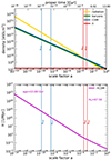 |
Fig. 1. Evolution of energy densities and expansion rate in the ΛCDM concordance model. Top panel: evolution of the energy densities, determined by Eq. (4). Bottom panel: evolution of the expansion rate H in natural units, determined by the total of the energy densities given by Eq. (5). The vertical lines in blue bracket the epoch of big bang nucleosynthesis, between neutron-proton freeze-out at an/p ∼ 1.3 × 10⁻¹⁰ and nuclei production anuc ∼ 3.3 × 10⁻⁹, while the vertical lines in red (at larger scale factor) indicate the time of matter-radiation equality aeq, followed by recombination arec, in terms of the scale factor a. |
3. Cosmic components with a time-dependent EoS parameter: The case for dark energy
While the current standard model ΛCDM is capable of modeling the expansion history of the Universe to good accuracy, certain discrepancies to data have been reported, such as the current value of the Hubble parameter, discussed below. More importantly, the very nature of Λ remains an open question, and the community has considered extensions to ΛCDM, which include the possibility of a DE component, in lieu of Λ, which comprises a time-dependent EoS parameter, the details of which depend on the underlying DE model. As a result, cosmological models are often fit to observational data, which include a DE component having a variable EoS parameter, while the concordance ΛCDM model with its constant wΛ = −1 is included as well. Prominent examples of observational campaigns which compare their data, among others, to individual DE candidates and a cosmological constant, include the CMB observations by Planck Collaboration VI (2020) and big galaxy surveys such as the DES-Y3 results (Abbott et al. 2022a). Both of them use the popular and useful CPL parametrization of Eq. (1). Similarly to the general solution known for a constant EoS parameter
the CPL parametrization of DE provides an analytical solution to the integration of the energy conservation Eq. (3), which reads as

This offers a very straightforward way to incorporate CPL-based models of DE into existing cosmological codes.
Before we present the details, we want to explain the consequences that arise from fixed EDs vs. fixed H0 in a more illustrative way in this section first. In order to discuss the evolution of the energy density and its contributing effect onto the expansion history of an exemplary component with a time-dependent EoS parameter, we compare it to the evolution of a component with a constant EoS parameter, sketched in Fig. 2.
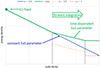 |
Fig. 2. Illustrative comparison between the evolution of energy density for a component with a constant or nonconstant EoS (arbitrary scaling). The blue component has a constant EoS parameter w = −0.8. The green component has a nonconstant EoS parameter w, which starts out with w = −0.8 (equal to the blue component) and evolves in two steps (indicated by the black vertical solid lines) to w = −0.9 (the slope is indicated by the dashed orange line) and finally to w = −1 (the slope is indicated by the dashed red line). The final density at the present time is higher for the green component. |
The initial density of the exemplary cosmic component is determined by processes in the very early Universe. Assuming that the EoS parameter remains constant, its evolution is shown by the blue solid line. Alternatively, we consider a case where an initially constant EoS parameter evolves to a different EoS parameter for this component (i.e., a time-dependent EoS), depicted by the green solid line. Obviously, for both cases the evolution is initiated at identical ICs. For the alternative with a time-dependent EoS parameter, we choose an EoS parameter that drops at two points in time (respective scale factors), first from w = −0.8 to w = −0.9 and finally to w = −1, the EoS parameter of a cosmological constant. With each drop the slope of the energy density evolution flattens (determined by the forward-integration of the energy conservation Eq. (3)). As a result, the final energy density at the present time is higher, compared to the energy density resulting from the assumption of a constant EoS parameter. Moreover, we recognize that a lower (higher) EoS parameter will decrease (increase) the deceleration of the expansion rate H, resulting in an increase (decrease) of H0, compared to a component described by a constant EoS parameter with identical ICs in the early Universe. We note that this simple illustration already indicates that a DE component with a decreasing EoS parameter could possibly provide an answer to the Hubble tension problem (in Wagner 2023, a different ansatz is presented, the result of which is comparable to our approach of forward-in-time integration, for it also provides a H0 closer to local measurements. They synchronize the cosmic time of early- and late-universe fits of cosmological models, indicating an increased expansion rate in the local Universe).
In contrast, we sketch in Fig. 3 examples of components which each have constant EoS parameter; where the case w = −1 describes the Λ-component in the ΛCDM model. No matter what the value for w is (blue, orange and red lines), the fact that w = const implies that the order of integration of the energy conservation Eq. (3) does not impact the final results, as the gradients of the densities never change. The fixed EDs approach vs. fixed H0 approach reveals no differences (without the need for a suitable choice of ICs for the backward integration). We can choose forward-in-time or backward-in-time integration, whatever may be suitable to our problem. In particular, we have this freedom in ΛCDM, where present-day density parameters Ωi, 0 and expansion rate H0 can be used in a backward-in-time integration of the energy conservation Eq. (3) for the energy densities of the individual components via the simplified Eq. (4). In effect, this procedure then determines the ICs in the early Universe, that represent the starting point for the evolution of the background densities, when the forward-in-time integration of the Friedmann equation in Eq. (5) is performed. This whole procedure is viable and leads to identical results for both approaches, as long as all components of a given cosmological model have a constant EoS parameter.
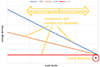 |
Fig. 3. Illustrative evolution of energy densities of components, each with constant EoS (arbitrary scaling). w = −0.8 (blue), w = −0.9 (orange), and w = −1 (red). |
However, once we introduce a component with nonconstant EoS parameter, such as a DE component in lieu of Λ, we need to be careful. Assuming initial densities to be determined in the early Universe and the fact that the Universe evolved from the early Universe to present, a component with a nonconstant EoS parameter, sketched by the green solid line in Fig. 2, requires a forward-integration of Eq. (3). So we cannot use the customary backward-integration, without a suitable choice of H0, as we exemplify below. Instead, integrating the energy conservation Eq. (3), starting from the initial densities in the early Universe up to the present, obtains the correct evolution of the densities, which enter the Friedmann Eq. (5). Related to this careful computation of the backward- and forward-in-time evolution is the choice of the correct starting point(s) of the integrations, depending on the corresponding cosmic time related to the measurement of H0, as we will elaborate shortly.
Although the Friedmann equation determines the expansion history as the total of the evolution of the energy densities over time (or scale factor) and eventually their initial values, it does of course not explain these initial values. The latter were determined by processes in the (very) early Universe and they impact the subsequent evolution of the background universe ever since, including the values at the present time. Although we cannot compute the EDs from first principles, in practice we can determine (or approximate) them by using observations which provide us with physical information at desirably high redshifts. These are foremost the observations of the CMB3, for example, by Planck Collaboration VI (2020), providing us with information on the density parameters for the constituents of the Universe at the time when the CMB has formed, that is the time of recombination at z ∼ 1090. Using these data extrapolated to the present, along with the choice of picking ΛCDM as our concordance model, we end up with a present-day value of the expansion rate of H0 ≃ 67 km s−1 Mpc−1. We may call it the “concordance value for H0”. By applying these parameters of the ΛCDM concordance model, we can compute the corresponding initial densities, these are the “concordance EDs”, now by the customary backward-in-time integration, that is fixing H0, as all constituents of the model have a constant EoS parameter. In the subsequent section, we will justify that these concordance EDs are indeed a very accurate way to determine the energy densities at place in the early Universe, making the fixed EDs approach feasible.
Furthermore, the evaluation of H0 in indirect observations (see e.g., Di Valentino et al. 2021) requires two steps. First, measurements of observables refer to a specific cosmic time, for example, the time when the CMB was emitted. Then, the implication of the measurement is extrapolated to redshift zero (see e.g., Alam et al. 2021), which is performed by assuming a specific cosmological model, for example, ΛCDM for the Planck-based H0. Extrapolated quantities, such as the value of H0, are bound to this specific cosmological model, used in the extrapolation. In turn, this concordance value for H0 implies respective concordance EDs, the values for the initial energy densities, and vice versa.
However, it is important to stress that this extrapolation step is not required for direct measurements of H0, for example, in the local Universe. Thus, these measurements are not sensitive to the choice of a specific cosmological model.
Now, we set up a general rule, illustrated in Fig. 4, how to compute the expansion history for components with time-dependent EoS parameter via integration of the energy conservation Eq. (3), in order to solve the Friedmann Eq. (5), such that the calculations are in agreement with the observed CMB spectra and lead to consistent results for the expansion history. When we apply the CMB-based determination of H0, it is the time of recombination arec (referred to as “CMB measurement” in the illustration), which shall be the starting point of the integration of Eq. (3): backward integration to get the energy densities prior to arec, all the way back to the very early Universe, and forward integration to get the energy densities at all later times past arec. On the other hand, if we choose a value of H0 determined by observations of the local Universe, when we may assume z ≈ 0, then the starting point for the integration is the present, and the integration of the energy densities is performed backward-in-time.
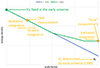 |
Fig. 4. Illustration of integration orders in determining energy densities of cosmic components. The actual ICs are fixed by processes in the very early Universe, but we have only access to observables at specific later times (respective redshifts or scale factors). The values of the latter determine the value of H, and by extrapolation to the present the value of H0. If H0 determined by the CMB is used, it is this starting point (referred to as “CMB measurement”) which must be used in the integration of Eq. (3): values for the energy densities before this point in time have to be calculated using backward integration, while values for the energy densities after this point in time have to be calculated using forward integration. The green component has a time-dependent w, while the blue component has a constant w = −0.8. |
To elaborate more on these rules, which we will adopt in the next section, we present two additional illustrations. The first one depicted in Fig. 5 displays a situation where the recombination time should be our reference point. Hence, we use the CMB-based value of H0. However, when we, as is customarily, fix H0 and apply a standard backward integration, using the present-day value of H0 extrapolated from CMB measurements, we “arrive” at “wrong” ICs, and not the ones which gave actually rise to the CMB that we measure. As a result, even a subsequent correctly performed forward integration of Eq. (3) will result in an “incorrect” evolution of the expansion history, not “fitting” to the CMB measurement4. The second illustration is shown in Fig. 6, and depicts a situation, where the present time is the reference point, using a value of H0 determined by observations of the local Universe. (These measurement values of H0 typically tend to be higher than those determined by the observation of the CMB, known as the Hubble tension problem, which we will discuss in the next sections). The reference point for the integration is now the present and we again fix H0. According to the rules, we now apply an integration backward-in-time ending up at the “correct” ICs, which determined the observed CMB temperature spectrum. A subsequent forward integration will then result in a correct evolution of the expansion history, as expected. We note that this result is in accordance with Fig. 2, where we fixed the early densities. A DE component with time-dependent EoS parameter can yield consistent results in both the fixed EDs and the fixed H0 computations of the expansion history, when the above mentioned rules, illustrated in Fig. 4, are met.
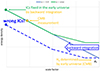 |
Fig. 5. Integration with wrong ICs. This illustration complements the one depicted in Fig. 4. The customary backward integration (blue dashed) of the green component with time-dependent EoS parameter leads to incorrect ICs, when we start from the value of H0 determined from observations of the early Universe. |
In the next section, we go beyond this qualitative picture and present detailed results for representative model universes having a DE component with a time-dependent EoS parameter, also known as a dynamical model of DE. The refinements to the computation procedure to include the fixed EDs approach, which we apply in the next section, can be summarized as follows.
If the “early” CMB-based extrapolation to H0 is used: computation of the EDs with the ΛCDM concordance parameters, because the reference point for the integration is the early Universe, and ΛCDM binds the concordance EDs to the concordance value for H0. This is followed by the forward integration, starting at the early universe with the computed EDs, using the parameters of the investigated model universe.
If the “local” value of H0 is used: backward integration, starting at z = 0 with the given value of H0, using the parameters of the investigated model universe.
4. Computation of exemplary cosmological models with dynamical dark energy
In this section, we make more precise our procedure, where we suggest to add a novel parametrization to cosmological codes, in order to perform the computations of the expansion histories of cosmological models, including components with time-dependent EoS. The novel parameter flags the provided value for H0 as inferred from measurements in the early Universe or in the local Universe, respectively, where early values of H0, according to our approach, demand fixed EDs and forward integration of Eq. (3), whereas local values demand fixed H0 and backward integration.
As already mentioned, early values of H0 require a two-step procedure. In the first step, we compute the EDs, that determined the observations of the configured value of H0 (e.g., the Planck-based value). In doing so, we must apply the same model parameters (e.g., the ΛCDM concordance values) that were used to extrapolate the observational data to the present-day H0, in order to arrive at the identical early densities, that evolved to those quantities that gave rise to the measurement values. The concordance EDs are bound to the concordance value for H0 via the ΛCDM concordance model, as we exemplified in the preceding section. The computation of the EDs corresponds to the illustration of Fig. 4, following the blue path from the present to the ICs in the early Universe. The subsequent integration follows the green path, where we have to forward-integrate the energy densities via the energy conservation Eq. (3) for each considered component, starting at the computed EDs, instead of using Eq. (4), by applying the parameters of the model under consideration, for example, a model with a dynamical form of DE. Obviously, local measurement values of H0 need no extrapolation of observational data to the present-day value of said H0. Hence, there are no special requirements on the computation of the EDs, but we have to perform a backward integration of Eq. (3), applying the parameters of the model under consideration. This corresponds to Fig. 6, where the computation backward-in-time and the subsequent forward-in-time integration follow the green path. In either case, the evolution of the background universe can be rightfully considered as an initial value problem (IVP), determined by the initial energy densities in the early Universe, which give rise to the configured value of H0 as determined by high-z or low-z observations, respectively.
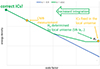 |
Fig. 6. Integration with correct ICs. This illustration complements the one depicted in Fig. 4. The customary backward integration of the green component with time-dependent EoS parameter “ends up” at the correct ICs, when we start from the value of H0 determined from observations of the local Universe. |
While we have emphasized the issue of consistent backward and forward integrations with respect to the adopted measurement value of H0 in models with time-dependent EoS, we must also stress another point. As a matter of fact, the data analysis of cosmological observations also often employ variations in the density parameters Ωi, 0, for example, variations in the matter content Ωm, 0, which are different from the values of the concordance ΛCDM model. This sampling of parameters is also related to the adopted routines, typically MCMC methods. Therefore, in highlighting our proposed procedure, we actually need to consider two different sources of variations in the parameters of a considered model universe: (1) at least one of the components has a time-dependent EoS parameter, as such a component is often used in the data analysis of cosmological observations, typically a DE component, and (2) the density parameters Ωi, 0 of components may be different from that model which was used in the extrapolation of H0 (i.e., different from the density parameters of the concordance model), as typically encountered in the MCMC data analysis of cosmological observations.
In our paper, we explore the impact of both sources of variations in the computations of model universes. To this end, we use the Boltzmann code CLASS5, which was designed to provide a flexible coding environment for implementing cosmological models, to calculate their background evolution and linear structure formation. The modular concept of CLASS and the coding conventions make it possible to enhance the existing code, without the risk of compromising existing functionality. Furthermore, it offers the configuration of a CPL-based DE component. The underlying code concepts can be found in Lesgourgues (2011). This code uses the “Planck 2018” cosmological parameters from Planck Collaboration VI (2020) as the default parameter set. Additionally, the configuration provides different sets of precision configuration files, to reflect varying requirements on precision needed in the results and available computation time. The precision configuration offering the highest accuracy is proofed to be in conformance with the Planck results within a 0.01% level.
We developed an amended version of CLASS, that includes our suggested enhancements in the procedure of computing the EDs and the integration of the energy conservation equation. The novel parametrization of an early-based (CMB) versus locally determined value of H0 makes sure that the corresponding switch is carried out in the computation of the EDs of the DE component and the subsequent integration of Eq. (3). If the parameter is flagged as early, the concordance ΛCDM parameters, that is the Planck-based value of H0 and the ΛCDM concordance parameters from Planck Collaboration VI (2020) are used (mentioned in the description of Fig. 1). If the parameter is set to local, then the calculation proceeds with the assumption that a locally determined value for H0 is being used. We used the CPL-based DE model in CLASS for the computation of the exemplary models presented in this section.
We first mention our results, concerning the impact of a variation of the (non-radiation) density parameters on the computation of model universes, in light of early and local values of the adopted value of H0. The bottom line is that we find no significant impact by our refined computational procedure, even for exotic models with very different values of Ωi, 0, compared to ΛCDM. Our computational scheme gives results not different from those applying the standard procedure. A marked difference only occurs, if the density parameter of radiation is changed. We relegate these results and their explanation into Appendix A. This, in fact, justifies the use of the concordance EDs as the early densities in our computations. This can also be seen in the figures we present in this section: regardless of huge variations in CPL model parameters, there are no deviations from the expansion history of ΛCDM at the time of recombination.
Now, our investigation of models having components with nonconstant EoS parameter, corresponding to the illustrations of the previous section, does reveal differences between our scheme versus the standard customary approach, when it comes to the late stages of the expansion history. We exemplify these differences by computing two different model universes with dynamical DE, applying the CPL parametrization (Eq. (1)). In the previous section, we recognized that an increasing or decreasing evolution of the EoS parameter with cosmic time determines a decrease or an increase of H0 compared to the evolution given by a constant w. For this reason we use two models. One model with an increasing EoS parameter and the second one with a decreasing EoS parameter.
The first model is inspired by the DES-Y3 results, having an increasing EoS parameter, that is wa < 0. In order to examine our suggested procedure, we are interested in probing the scheme for models which differ from the concordance ΛCDM model, if ever so slightly. We considered first a comparison of the results of DES-Y3 with ΛCDM, as follows. We stress that DES-Y3 is in accordance with ΛCDM to within 1-σ. But they investigate also the CPL model of DE (see Eq. (1)) and find values of  and
and  . We used the mean values of these parameters to describe a cosmology with DE and call it the DES-Y3 CPL model for simplicity. For these CPL mean values, the EoS of DE evolves from an initial value of wDE = −1.35 to a final value of wDE = −0.95, that is a model with increasing EoS parameter.
For the second model we used a decreasing EoS parameter, that is wa > 0. While the DES-Y3 and Planck results prefer a nonpositive value of the CPL parameter wa clearly below zero (for DES-Y3 see Abbott et al. 2022a, their Fig. 4, the light blue contours and the red contours, where they include data from Planck Collaboration VI 2020, Fig. 30; only the combination with low-z data, seen in their Fig. 5 green contours, shifts the result to the “less negative” value wa = −0.4), other observations in the more local Universe show a preference for a positive value of wa, that suggests a decreasing w for DE. For example, BAOs measured in the SDSS Data Release 9 spectroscopic galaxy survey by Anderson et al. (2012), in addition with measurements of luminosity distances from a large sample of SNe Ia by Guy et al. (2010), Conley et al. (2011), and Sullivan et al. (2011) yield  and
and  (Hinshaw et al. 2013). Such as with DES-Y3, the results are statistically in agreement with ΛCDM; in the case here a cosmological constant is within the 95% confidence region in the w0 − wa plane. So, given the possibility of discrepant preferences for the CPL parameters of DE from different cosmological observations, we also present the analysis of our computational scheme for models with positive value for wa, that is a decreasing EoS parameter. As a case in point, we used the following CPL parameters, w0 = −0.9 and wa = +0.1, for which the EoS parameter evolves from wDE = −0.8 to a present-day value of wDE = −0.9. This choice is substantiated by inspection of Fig. 5 of the DES-Y3 results in Abbott et al. (2022a), where the green contours in that figure show low-z data alone. For these data, the probability of a cosmological constant is right at the edge of the 1σ-area. Moreover, the center of this area is such that w0 lies above −1 and wa is clearly larger than zero, thus also preferring DE over a cosmological constant.
4.1. Standard procedure
We started with the computation of both models using the standard computational procedure, that is fixed H0, shown in Fig. 7; the left-hand side displays the results for the DES-Y3 CPL model; the right-hand side those for the CPL model with wa > 0. Both models are compared to the ΛCDM concordance model.
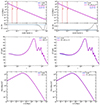 |
Fig. 7. CPL models (magenta) and ΛCDM (blue) both computed with the standard procedure. The left-hand side displays the results of the DES-Y3 CPL model with w0 = −0.95 and wa = −0.4. The right-hand side displays the results for the CPL model with w0 = −0.9 and wa = +0.1. We use the original version of CLASS and the value of H0, determined by CMB observations from Planck Collaboration VI (2020). The top panels display the expansion histories, where the vertical lines in red indicate the time of matter-radiation equality at scale factor aeq, followed by recombination arec (both determined by the cosmological model). The bottom insets show the relative deviation of the respective expansion histories (gray curve), which only matters at late times (respective high scale factors). The middle and bottom panels show the CMB temperature spectra (temperature anisotropies) as a function of mode number l, and the matter power spectra as a function of wave number k, respectively. |
4.1.1. Standard procedure (increasing w)
The expansion history of the DES-Y3 CPL model, compared to ΛCDM, is shown in Fig. 7 top left-hand panel. We used the original CLASS code with the default value of H0 = 67.56 ± 0.42 km s−1 Mpc−1, obtained by Planck Collaboration VI (2020, see their Table 2, column “TT, TE, EE+lowE+lensing”, where CLASS additionally uses a best fit to WMAP data). As expected from the fixed H0 approach, we see an almost perfect agreement with the expansion history of the ΛCDM model, and only at late stages, beginning at a ∼ 10−1, a decrease in the expansion rate of the CPL model of ∼1% compared to ΛCDM is seen. It subsequently overshoots the expansion rate of ΛCDM, and finally is forced back (!) to the configured value of H0 (see the gray line at the bottom of the panel), as we have fixed H0 and the densities in the early universe are then given by the model. Also, the calculation of the CMB temperature spectrum (middle panel) and matter power spectrum (bottom panel) in the left-hand side column displays a perfect agreement with ΛCDM.
Considering the illustration of Fig. 5, where the customary computational procedure (by fixed H0) arrives at the wrong early densities, one may be surprised to see such a perfect agreement with ΛCDM. Nevertheless, the explanation for the perfect agreement, in expansion history as well as in the spectra, is straightforward and can be illustrated partly with the top panel of Fig. 1, which displays the evolution of the energy densities in ΛCDM. We recognize the well-known fact that Λ remains a very subdominant component well past arec. Of course, the same is true for the DE component of the DES-Y3 CPL model: although its density (not shown) is not a constant line, it is also very much subdominant compared to the other (early) densities. The spectra are in agreement with ΛCDM, also thanks to the expansion history, being “forced” to the configured value of H0. This is supported by the findings of Vagnozzi (2023), stating that modification of physics beyond ΛCDM in the early Universe is not sufficient to resolve the Hubble tension.
4.1.2. Standard procedure (decreasing w)
Similarly to the DES-Y3 CPL model, we show in the right-hand side column of Fig. 7 the results for the CPL model with a positive wa, using the Planck-based value of H0 in the standard procedure. We again compare these results from the public version of CLASS with ΛCDM. The top panel displays the expansion history. We recognize again an almost perfect agreement with ΛCDM. However, beginning with a ∼ 10−1, the expansion rate in the CPL model increases to ∼3% above the value of ΛCDM at a ∼ 6 × 10⁻¹, but subsequently is forced back (!) to the configured value of H0. Also, we show the CMB temperature spectrum and the matter power spectrum computed with the standard procedure, in the middle and bottom panel, respectively. For reasons already mentioned for the DES-Y3 CPL model, we see an almost perfect agreement with ΛCDM.
4.1.3. Conclusions for the standard procedure
Given the subdominance of a DE component in the early Universe, the deviation in the total sum of densities compared to the one with Λ is small, resulting in negligible deviations in the early expansion history. On the other hand, in the late stages of expansion, the customary computational procedure is insensitive to the evolution of w (see e.g., Ó Colgáin et al. 2021; Staicova & Benisty 2022; Vagnozzi 2023), as the impact of wa converges to zero and H0 is forced to the configured value. This explains why we do not see a decrease in H0, in contrast to the expectations from Fig. 2 for an increasing EoS parameter. Hence, we see that the computational procedure applied to the CPL-parametrized DE component is insensitive to the parameter wa.
We performed an additional test, and computed a model with negative wa, using (DES-Y3)-only data; see the light blue contours in Fig. 4 of Abbott et al. (2022a). We used the (mean) values w0 = −0.6 and wa = −1.8, corresponding approximately to the central point of the 1σ-region. These values are clearly different from w0 = −1 and wa = 0 of a cosmological constant. Yet, we received results in almost perfect agreement with ΛCDM for the expansion history, the CMB temperature spectrum and the matter power spectrum. We draw the conclusion, that the standard computational procedure, not only is insensitive to the parameter wa, but there is a severe w0 − wa-degeneracy. In fact, given the Planck value of H0, one can find probably an infinite number of combinations of w0 and wa, including the one of a cosmological constant, that perfectly match the CMB temperature spectrum, where the density parameters for radiation, CDM and baryons remain unmodified. We also recognize that DES-Y3 use the density parameters obtained from the base cosmology, while using w0 and wa in the list of priors, when fitting the CPL model.
In fact, we computed three models with DE components that clearly are different from ΛCDM, and all of them are in perfect agreement with the CMB temperature spectrum. Consequently, we may conclude, that the mere agreement with the ΛCDM concordance model, due to the w0 − wa-degeneracy, does not by itself confirm the cosmological constant Λ. Hence, the Planck value of the Hubble constant H0 cannot be considered as a unique value. But it is simply the value determined by the assumption of a cosmological constant, that is w0 = −1 and wa = 0 (and the flatness of space). This degeneracy in the customary computation procedure, exemplified here for the CPL parametrization, exists for any kind of dynamical model of DE.
Moreover, the inability of discriminating CPL models in terms of the parameters wa and w0 affects the results when fitting CPL models to observational data. This eventually provides an explanation for the aforementioned unspecific results of data analyses, for values of wa above and below zero; see also Dainotti et al. (2023b,c) and Bargiacchi et al. (2022), which report the same nonpositive values for wa, as seen in DES-Y3 (Abbott et al. 2022a) and Planck Collaboration VI (2020).
4.2. Amended procedure
We proceeded with the same model comparison, CPL model versus ΛCDM, but this time applying our complimentary computational procedure by employing the choice of using “early-based” and “locally based” values for H0, parameterized according to our amended version of the CLASS code. In order to break the w0 − wa-degeneracy of the standard procedure, an additional assumption is needed. We will exemplify below that the expansion rate H in the early Universe is a viable quantity to break the degeneracy, as it is approximated to high accuracy by the ΛCDM concordance model, which is immune to the w0 − wa-degeneracy. We performed this comparison for both CPL models; first for the DES-Y3 inspired model with increasing w and then for the model with decreasing w.
4.2.1. Amended procedure (increasing w)
The results for the DES-Y3 CPL model are shown in Fig. 8. We make a side-by-side comparison of the plots, using the early CMB-based H0 = 67.56 ± 0.42 km s−1 Mpc−1 from Planck Collaboration VI (2020), that is the fixed EDs approach (left-hand column), and the locally based, that is the fixed H0 approach (right-hand column) using H0 = 73.04 ± 1.2 km s−1 Mpc−1 from Riess et al. (2022). Top panels show the expansion histories, and the middle and bottom panels show the CMB temperature and matter power spectra, respectively. Let us first focus on the top panels. The top-left panel depicts the results for the CMB-based value of H0. According to the nonpositive parameter wa of the CPL model for DE, we clearly see a significantly decreased value of H0 = 48.68 km s−1 Mpc−1, compared to the configured value H0 = 67.56. Of course, that value for H0 is not in agreement with observations, but in light of the expectation from Fig. 2, we can understand what happened: the increasing EoS parameter results in a decrease of H0 toward the present time. Again, around arec, there is no difference between the DES-Y3 CPL model and ΛCDM, for both Λ and DE are then subdominant. The top-right panel shows results for the locally based value of H0. The relative evolution of H in the DES-Y3 CPL model displays a slight s-shape (gray curve in the inset). This calculation corresponds to the situation illustrated in Fig. 6, where the backward integration arrives at the correct EDs.
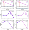 |
Fig. 8. DE component with increasing w: the DES-Y3 CPL model with w0 = −0.95 and wa = −0.4 (magenta) compared to ΛCDM (blue), both computed with our scheme. Panels on the left-hand column were computed using the early parametrization of H0 = 67.56 km s−1 Mpc−1 using Planck Collaboration VI (2020), while panels on the right-hand column employ the local parametrization of H0 = 73.04 km s−1 Mpc−1 from Riess et al. (2022). Top panels: expansion histories; for the vertical lines in red see Fig. 7. We note the deviations in the expansion histories from ΛCDM at late times (respective high scale factors) and the different run of these deviations (see gray curves in the bottom insets of the top panels). Middle panels: CMB temperature spectra. Bottom panels: matter power spectra. The results based on the CMB-determined H0, shown in the left-hand column, display a clear deviation from ΛCDM, whereas the results based on the locally determined H0 are in better agreement with ΛCDM. |
The spectra in the left-hand column also display clear deviations from ΛCDM, due to the deviation of the expansion history in the late Universe. While the peak structure in both cases is barely affected (as the density parameters of radiation, CDM and baryons are identical to ΛCDM), there is an overall shift, horizontally for the CMB spectrum and vertically for the matter power spectrum, due to the reduced growth of structures in the late stages of the evolution, for the latter. The horizontal shift to the right-hand side in the temperature spectrum is connected to the deviation in the expansion rate, as follows. The multipole moments shown in the x-axis, are in Fourier space. Hence, it is not a shift, but stretching (compressing) of the spectrum from the right-hand side to the left-hand side, with increasing (decreasing) expansion rate. More pronounced differences in the spectra occur at large spatial scales (corresponding to low l and low k, respectively).
Comparing now to the right-hand column, which uses the local value of H0, we see much better agreement with ΛCDM for all observables, although some minor deviations in the spectra remain at large spatial scales (probably of no discriminating significance given the error bars of CMB measurements at low l). As mentioned earlier, this outcome corresponds to Fig. 6, where the backward-in-time integration arrives at the correct densities in the early Universe.
To reiterate, the simulation run for the early-based (high z) value of H employing our scheme does not force the expansion rate to the configured concordance value of H0 = 67.56 km s−1 Mpc−1, as we have fixed the early densities while H0 is determined by the (CPL) model. Therefore, we see “exacerbated results” on the left-hand column, with H0 = 48.68 km s−1 Mpc−1, compared to the standard procedure depicted in Fig. 7. But in light of the explanations of Fig. 2, we conclude that the results of the amended procedure are correct, that is more realistic in terms of the physical expectations. On the other hand, the results displayed in the right-hand column conform much better to ΛCDM, because our starting point in the backward integration uses the locally based H0 (at z ≈ 0), which is numerically close to the concordance value for H0 to begin with. Yet, the two simulation runs using different H0, depending on whether early-based or locally based measurement values have been used to parameterize the integration runs, do not display consistent results for the two approaches of fixed EDs vs. fixed H0; we see clear differences between the left and right columns in Fig. 8, signaling that backward and forward evolution of the expansion history does not yield consistent results. Therefore, this model is not able to provide an answer to the Hubble tension problem.
4.2.2. Amended procedure (decreasing w)
Now, Fig. 9 proceeds with the comparison of the other considered CPL-DE model with wa > 0 vs. ΛCDM, computed by the amended procedure. We make a side-by-side comparison of the plots, using the early CMB-based H0 = 67.56 ± 0.42 km s−1 Mpc−1 from Planck Collaboration VI (2020), that is the fixed EDs approach (left-hand column), and the locally based, that is the fixed H0 approach (right-hand column) using H0 = 73.04 ± 1.2 km s−1 Mpc−1 from Riess et al. (2022). In the top panels, we see the expansion histories. Again, the expansion rate displays no difference to ΛCDM around and well past arec. For the early-based value of H0, we see beginning at a ∼ 10−1 a rise of H resulting in H0 = 75.25 km s−1 Mpc−1, in contrast to the concordance value H0 = 67.56 km s−1 Mpc−1. This result is in agreement with the expectation from Fig. 2 that a decreasing EoS parameter w leads to a higher Hubble constant at the present, when fixing the early densities. On the other hand, the right-hand panel uses the local value of H0 = 73.04 km s−1 Mpc−1 from Riess et al. (2022). As expected and similarly to the right-hand column of the previous Fig. 8, the resulting value of H0 is identical to the configured value, as this is the starting point for the backward integration, when fixing H0 (see Fig. 6), to determine the evolution of the energy densities. The comparison of the CMB temperature spectra and the matter power spectra obtained from the amended computational procedure, using early vs. local values of H0, with ΛCDM are also depicted in Fig. 9. For both spectra, we see good agreement with ΛCDM, except for some deviations at large spatial scales.
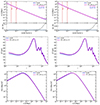 |
Fig. 9. DE component with decreasing w: a CPL model with w0 = −0.9 and wa = +0.1 (magenta) compared to ΛCDM (blue), both computed with our scheme. Panels on the left-hand column were computed using the early parametrization of H0 = 67.56 km s−1 Mpc−1 from Planck Collaboration VI (2020), while panels on the right-hand column employ the local parametrization of H0 = 73.04 km s−1 Mpc−1 from Riess et al. (2022). Top row: expansion histories; for the vertical lines in red see Fig. 7. Middle panels: CMB temperature spectra. Bottom panels: matter power spectra. In both columns, we see good overall agreement with ΛCDM, except for the fact that the chosen CPL model may provide a resolution to the Hubble tension problem. A difference remains in the present-day Hubble constant between left-hand and right-hand columns, see main text. |
Again, the amended code gives us results for the expansion histories, as well as for the spectra, with respect to the different (local vs. early) parametrizations of H0, which are in accordance with the expectations described in Sect. 3. In contrast to the model with an increasing EoS parameter, we see here, for the model with a decreasing EoS parameter, consistent results for each case, fixed EDs or fixed H0, along with being in accordance with observations across cosmic time. We might thus conclude that this model points toward a resolution to the Hubble tension problem. Of course, more precise statements require further investigation, for example, provided via an extended MCMC analysis as discussed in Sects. 5 and 6.
4.2.3. Conclusions for the amended procedure
Summarizing the results of the two CPL-based DE models in this section, Figs. 8 vs. 9, we can see that the latter case – a CPL-DE model with wa > 0, that is a decreasing EoS parameter – gives much better agreement with both, the concordance ΛCDM model and the present-day locally determined Hubble constant from Riess et al. (2022). In other words with each, either fixed H0 or fixed EDs, respectively, via the backward and forward integrations of this CPL model of Fig. 9 yield results which are (much more) consistent with observations, compared to the model in Fig. 8. In principle, we could attribute this finding to the mere chance of having picked favorable CPL parameters (were it not for other reasons which motivated our choice in the first place; a publication on a physics-based model of DE is currently in progress). Indeed, the CPL parametrization is purely a convenient way of representing DE models with a time-dependent w, and it is not obvious that any choice of its free parameters will fit perfectly to observations (see e.g., Ó Colgáin et al. 2021; Dinda 2022). However, it so happens that a choice of w0 = −0.9 and wa = +0.1, upon fixing EDs, yields a value of H0 = 75.25 km s−1 Mpc−1, which is quite close to the value of Riess et al. (2022; which is the starting point of the backward integration in each model that we calculated).
We can draw two major conclusions from this section. First, our results suggest that a DE component with a decreasing EoS parameter w may provide a resolution to the Hubble tension problem, because the results of both backward-in-time (fixed H0) and forward-in-time integrations (fixed EDs), each with their respective flagging of H0 (early or local), are in good agreement with the local measurements of H0 and the expansion rate at the time of recombination. Second, we argue that the requirement of finding consistent results in both cases should be used as a restrictive criterion of cosmological models. In fact, the procedure can help to find model parameters that are free of the Hubble tension problem, in a very natural way, in that they also provide a present-day Hubble constant in accordance with local measurements. In the next section, we discuss how this approach should be implemented via a three-step procedure in a kind of extended MCMC method, that is such that eventually only models without any difference between forward and backward, (i.e., fixed EDs and fixed H0) evolution will be sampled, while being in agreement with local measurements. We expect that such an approach will considerably increase the determined accuracy of the parameters of cosmological models; see also e.g. Dainotti et al. (2021, 2022a,b, 2023b), Bargiacchi et al. (2023a,b), Ó Colgáin et al. (2021), Staicova & Benisty (2022), Krishnan et al. (2021), and Łukasz Lenart et al. (2023) whose results indicate that measurements (up to z ∼ 7.5 using quasars) might favor a dynamical model of DE.
More precisely, with regard to the computation of cosmological models and in light of the conclusions for the standard procedure of Sect. 4.1.3, we demand consistent results in the computation of a cosmological model, obtained from early densities approximated by concordance ΛCDM values (fixed EDs approach) with those obtained via H0 as measured in the local Universe (the customary fixed H0 approach), which breaks the w0 − wa-degeneracy and fulfills the general requirement to give consistent results in the forward and backward evolution of the model and being in agreement with observations. Consequently, in addition to the above CPL-based DE models, we performed this consistency check for ΛCDM, where we used our amended code with a CPL parametrization, that is setting w0 = −1 and wa = 0, using the early vs. local parametrization of H0, respectively. Unsurprisingly, we recognize a Hubble tension problem in the concordance ΛCDM model, see Appendix B.
5. Toward an improvement of the accuracy of cosmological observables
In the previous sections, we discuss our complementary approach of fixed EDs vs. the customary approach of fixed H0 in the computations of cosmological models with a DE component having a time-dependent EoS, and we present a refined procedure for the self-consistent computation of the expansion history and linear spectra. In this section, we advance one step further and we argue that under the assumption of a cosmological origin of the Hubble tension, the very requirement of recovering consistent results between backward-in-time (i.e., fixed H0) and forward-in-time (i.e., fixed EDs) evolution of cosmological models should be used, in order to check the consistency of a cosmological model (see also Appendix B and Sect. 4.2.3). This consistency check, in turn, can be used to extend the standard MCMC procedure used to analyze cosmological data. As a result of this requirement, we expect the available parameter space to be significantly reduced, leading to an increase in the accuracy of the derived parameters of cosmological models, in particular for extensions to ΛCDM.
The Hubble tension problem basically refers to the discrepancy in the measurement results for H0 between observations of the CMB – whose analysis is based on extremely well-understood theories – and observations in the local Universe – based on extremely well-checked measurements. Generally, the latter provide higher values of H0 than the CMB-based extrapolated values for H0 (see e.g., Hu & Wang 2023). At the same time, from a theory perspective, we require consistent results for model universes evolved from the early Universe to the present and vice-versa from the present to the early Universe, while being in agreement with observational data across the entire expansion history. In Appendix B, we highlight the case of ΛCDM as an example to check the consistency of cosmological models and their parameters, respectively. This procedure is built on the assumption that the evolution of the background universe is a well-posed IVP, describing the evolution from the early Universe to the present (fixed EDs approach). However, the same shall be true in the converse direction (since we consider the Universe as a closed and conservative system), that is using ICs provided by measurements of the local (present) Universe, the equations of motion can be evolved backward-in-time to the early Universe (customary fixed H0 approach), for example, back to the time of recombination, yielding identical results to the forward evolution.
The question arises as to how the consistent treatment of both approaches can be combined in the analysis of cosmological data. In general, cosmological observations, that apply the MCMC method, explore the parameter space of (typically) FLRW models, and determine the probability distribution of each of the model parameters, by “matching” the properties of computed model universes to observational data. For example, the data analysis of DES-Y3 match the computed matter power spectra with observed BAO data, in order to determine the set of model parameters with the highest likelihood. The CMB observation by the Planck mission uses a similar procedure: computed temperature spectra are matched with the measured CMB spectrum, yielding the set of model parameters with the highest likelihood, the well-known concordance parameters of the ΛCDM model.
Now, we already emphasized that many observational campaigns (such as DES-Y3, or the Planck mission) include in their analysis (i.e., in their comparison with data) candidates for DE with a time-dependent EoS parameter via a CPL parametrization (see Eq. (1)), along with the cosmological constant of ΛCDM. Since these candidate models are affected by some issues identified in the previous section (see Sect. 4.1), when only the customary fixed H0 approach is applied, we suggest that the aforementioned consistency check, based on the fixed EDs approach, is being applied, in order to avoid these issues. As a result, we expect that the viable parameter space of models shrinks dramatically, as for example, dynamical models of DE with an increasing EoS parameter will probably be ruled out, such that a significant improvement in the accuracy of the determined parameters of cosmological models can be achieved. The standard MCMC computational method should be extended to include a three-step procedure, where each step applies the refined computational procedure introduced above, as follows.
First, we remind that in the standard MCMC method each of the model parameters is assigned a presumed range of values (known as the priors), that determine the entire parameter space of a given model to be fitted to data. The parameter space (i.e., a grid of parameter sets) is sampled iteratively, advancing from one parameter set to the next. In each step, the model is computed (comparable with our model computations in the preceding section) and matched to observational data. The quality of this match is expressed by computing the likelihood, for example, by a χ-square test. The likelihood controls the strategy of the sampler, which also assures not to step out of the defined parameter space but to remain within it. In a final step, the probability distribution (known as the posterior distribution) is computed, applying Bayesian statistics. We propose to extend the computational step for the sampled models to a three-step procedure, instead of the standard two-step procedure.
In the first step, the cosmological model under consideration (by the sampler) is computed using the value of H0, inferred from measurements or sampled as a member of the priors, respectively, now flagged as local, performing a backward integration of the densities, starting from the local ICs, as demanded by the fixed H0 approach (this corresponds to Fig. 6). Keeping the w0 − wa-degeneracy in mind, one must not restrict the prior of H0 by for example, including probability densities from previous literature or previous computations with restricted parameter space, etc. (see e.g., DES-Y3 results for the w0 − wa model).
The novel second step introduces the fixed EDs approach. In this step, the sampled cosmological model is computed according to the fixed EDs approach by applying the concordance value for H0 (flagged as early) and the concordance model parameters. We note that these model parameters are not those determined by the MCMC method. They do not enter the lists of priors and posteriors. They only determine the initial densities, as demanded by the fixed EDs approach (this corresponds to Fig. 4). Starting at these computed EDs, the subsequent forward integration applies the sampled parameter set, entering the computation of the posteriors.
The final step also extends the customary procedure of the MCMC analysis. While customarily, the sampled model parameters are fitted to the measured data (e.g., CMB temperature spectrum or the matter power spectrum, respectively), we now consider all information available for the sampled model: the expansion histories, CMB temperature and matter power spectra from the computations. Both results, from fixed H0 (step one) and fixed EDs (step two), are checked for consistency. Only those parameter sets, that display consistent results for all three quantities, taking the accuracy of the measurements into account, are considered in the subsequent computation of the likelihood and the probability distribution, respectively. Since this additional consistency check will lead to a reduction of the allowed parameter space (probably ruling out dynamical models of DE with an increasing EoS parameter, see also next paragraph), it will increase significantly the accuracy of the final parameters, resulting from the MCMC analysis.
Encouraged by the results depicted in Fig. 9 for a DE component with decreasing EoS parameter, that is wa > 0 in the specific CPL parametrization, we see the Hubble tension problem to be explained phenomenologically in a very natural way by applying the fixed EDs approach. We expect, based on the proof-of-concept implementations in the preceding section, that such an analysis will find w0 > −1 and wa > 0, which is in agreement with low-z data depicted by the green contours in Fig. 5 of DES-Y3 (Abbott et al. 2022a). Also, Y1 results presented in Fig. 11.13 of LSST Science Collaboration (2009) depicts a probability distribution in the w0 − wa-plane compatible with our expectation. In contrast, DES-Y3 results (Abbott et al. 2022a) and the CMB measurements by Planck Collaboration VI (2020), when comparing a CPL-based model of DE to a cosmological constant, yield a high probability for wa < 0 (see also Dinda 2022; Vagnozzi 2023; Ó Colgáin et al. 2021; Staicova & Benisty 2022). Our calculation of an exemplary model in Sect. 4.2.1 with wa < 0, where we picked their central values of the CPL parameters calling it DES-Y3 CPL model for mere convenience, does not pass the recommended consistency check (see Fig. 8).
In the description of step one of the extended MCMC routine, we argued that one must be careful when including information from previous measurements into the Markov chain, in order not to anticipate a value for H0. Of course, using results from previous observations is an important means to improve the accuracy of one’s own data analysis. But instead of including previous probability distributions, we did this by including the measured CMB temperature spectrum in the computation of the likelihood in step three by comparing it to the computed temperature spectrum of the sampled model. To this end, we implemented a proof-of-concept version of the extended MCMC procedure and fitted our model with w0 = −0.9 and wa = +0.1 to the CMB temperature spectrum of the concordance model using our amended version of CLASS. The resulting parameters w0 = −0.875 and wa = 0.075 removed the minimal horizontal shift of the spectrum, seen in Fig. 9 and gives a perfect agreement with the measured spectrum (with the concordance ΛCDM model, respectively).
Finally, we stress again that the cosmological model, which is used in deriving extrapolations of observables, such as H0, is bound to these values. In other words, the EDs giving rise to the CMB measurements, the extrapolated H0 and the corresponding cosmological model (parameters) are inextricably linked together, where none of them can be used without being impacted by the other. This fact also explains results of indirect measurements, which (apparently!) seem not to apply CMB-based measurements, and yet yield values of H0 close to the Planck concordance value, as seen for example, in Fig. 1 by Di Valentino et al. (2021). Such a case can be seen in Alam et al. (2021), their Table 5 with H0 = 67.35 ± 0.97 km s−1 Mpc−1, based on Big Bang nucleosynthesis (BBN) and BAO data. They apply the MCMC method, while using Ωr, 0 from the concordance model (thus, excluding radiation from the MCMC-sampled parameter space), and assuming a cosmological constant. Hence, the computations of the sampled cosmological models as part of the MCMC method arrive at a value of H0 close to that of the concordance model (see also Appendix A). In this sense, the use of CMB data is implicit in these mentioned cases, due to the relation between the concordance ΛCDM model, H0 and the corresponding initial densities, that have been implicitly applied in their model assumptions, namely Ωr, 0 of the concordance model and a cosmological constant. As this could be seen as a bad example of the characteristics connected to the customary fixed H0 approach, it confirms at the same time our approach to approximate the initial densities in the early Universe as determined by the ΛCDM concordance model.
6. Summary and conclusion
A cosmological model should fulfill certain criteria. First, computations of the model forward-in-time and vice versa backward-in-time must yield identical results. Consistent results in forward and backward evolution of a model basically checks the consistency of the computation and not of the model. Apart from some exotic models of cosmic components, this is not an issue in the computation of the expansion history. The second condition is even more important: the results have to agree with observations across cosmic time. In this sense, the ΛCDM model is not consistent, for it does not agree with local measurements of the Hubble constant (Hubble tension problem). On the other hand, in the early Universe, ΛCDM is in conformance with measurements of the CMB. Recent studies analyzing the evolution of the expansion rate H at low redshifts indicate that these data are not in accordance with a cosmological constant and that the Hubble tension might be of cosmological origin, due to a DE component with a time-dependent EoS parameter, rather than connected to issues in the local measurements (e.g., Krishnan et al. 2021; Dainotti et al. 2023a; Khalife et al. 2024).
In Sect. 3 we discuss in a qualitative way if the customary computation procedure for the expansion history of a cosmological model can be applied to a DE component with a time-dependent EoS parameter. We find that special considerations must be taken into account, compared to a component with a constant EoS parameter. We conceived a refined procedure to compute the evolution of the energy densities, in that we implemented a case distinction between the provided H0 from measurements based either on the early Universe (CMB-based), or the local Universe (e.g., based on standard candles). Most important, we find that the concordance EDs, computed by the customary backward-in-time integration starting at the concordance value for H0, provides an accurate approximation of the initial densities in the early Universe. These are used as the starting point for the subsequent forward-in-time integration of the energy conservation Eq. (3). Hence, for early-based values of H0, the required forward-in-time integration starts at the computed early densities, whereas for locally based values of H0 the integration is performed backward-in-time.
In Sect. 4 we implement this computation procedure into the code CLASS and perform computations of the expansion histories, CMB spectra and matter power spectra of representative cosmological models. Hereby, we find that the customary computation procedure, fixed H0, for the expansion history of a cosmological model is affected by a w0 − wa-degeneracy of the CPL parametrization applied to the DE component, that is due to the subdominance of DE in the early Universe while becoming dominant only in the late Universe. We show in Sect. 4.1 that this degeneracy results in an agreement with ΛCDM over a wide range of the parameters w0 and wa. In fact, this degeneracy applies not only to the CPL parametrization, but to all dynamical models of DE which offer the same degrees of freedom in the evolution of w(z). For Planck-based value of H0, one can find a number of combinations of w0 and wa that result in an agreement with ΛCDM. This biases the fitting of models to data, as well (Dinda 2022; Vagnozzi 2023; Ó Colgáin et al. 2021; Staicova & Benisty 2022). It also explains the nonpositive values for wa reported in the DES results (Abbott et al. 2022a and Planck Collaboration VI 2020); see DES-Y3 in Abbott et al. (2022a) and the light blue contours and the red contours in their Fig. 4, where they include data from Planck Collaboration VI (2020), Fig. 30. Only the combination with low-z data, seen in their Fig. 5 green contours, shifts the result to the “less negative” value of wa = −0.4, compatible with a cosmological constant.
In Sect. 4.2, we propose and analyze a complementary computational approach – the fixed EDs approach – for the computation of the expansion histories for cosmological models, that breaks the w0 − wa-degeneracy, affecting dynamical models of DE with a time-dependent EoS parameter. This approach is built on the assumption that the evolution of the background universe is a well-posed IVP, describing the evolution from the early Universe to the present, given by initial densities in the early Universe, determined by processes at play prior to the cosmic time, where the computation of the cosmological models is initiated. Although we cannot determine the initial densities at place in the early Universe from first principles, we can use the fact that the initial densities are approximated by the ΛCDM concordance model, applying the customary fixed H0 approach, with high accuracy, as ΛCDM with its constant w is not affected by the w0 − wa-degeneracy. As a result, the fixed EDs approach can eventually provide a possible resolution to the Hubble tension problem by a DE component with a decreasing EoS parameter, under the assumption that the Hubble tension is of cosmological origin and not based on issues in the local measurements. We find that the model with decreasing w(a) = − 0.9 + 0.1(1 − a) comes close not only to a consistent evolution, when backward-in-time (fixed H0) and forward-in-time (fixed EDs) calculations are compared to each other, but it also predicts a present-day value of the Hubble parameter close to that inferred by observations of the local Universe. Thus, such a DE model may provide a resolution to the Hubble tension problem (see also Fig. 2 for illustration). In contrast, the model with increasing w(a) does not display a consistent evolution, when backward-in-time (fixed H0) and forward-in-time (fixed EDs) calculations are compared to each other.
In short, the two approaches can be characterized as follows. The customary fixed H0 approach starts the computation at the present with a given value of H0 and integrates the equations backward-in-time toward the early Universe. Thus, the densities in the early Universe (and thereby H(z)) vary with the choice of the model and its parameters. Instead, the fixed EDs approach starts the computation in the early Universe with initial densities determined by the ΛCDM concordance model, being identical for all considered models. We found these densities to approximate the “real” densities to high accuracy, making this approach feasible. Thus, the densities at the present (and thereby H0), determined by a forward-in-time integration of the equations, vary with the choice of the model and its parameters. The important difference between both approaches is that in the fixed EDs approach the resulting H0 can be checked (and is checked) against observations in the local Universe. Whereas, in the customary fixed H0 approach H(z) in the early Universe is not checked against observations in the early Universe. In addition, as exemplified in Sect. 4, due to the subdominance of DE in the early Universe, it is not promising to perform those checks. Moreover, the customary fixed H0 approach is, by construction, not able to provide an answer to the Hubble tension problem, regardless of the model tested. Hence, it rules out a cosmological origin of the Hubble tension problem by construction, relegating it to issues in the local measurements.
We like to stress that our fixed EDs approach is no criticism of the correctness of H0 as determined by Planck Collaboration VI (2020). On the contrary, the assumption of a cosmological constant was the only reasonable choice at the time of measurement, and moreover, is immune to the consequences of a dynamical model of DE. We simply treat it what it is: the information of conditions at place at a redshift of z ∼ 1090 extrapolated to present-day values, under the assumption of a cosmological constant6. Only the existence of these results makes the fixed EDs approach feasible. In other words, the finding of the concordance EDs is the great achievement of the CMB measurement by the Planck mission, with the establishment of the ΛCDM concordance parameters.
Subsequently to the finding of Sect. 4.2, we argue that employing both, fixed EDs approach and fixed H0 approach, provides a consistency check for cosmological models. In Sect. 5 we propose that this novel consistency check be included in the standard MCMC method, that is applied in many observational programs to compare dynamical models of DE to a cosmological constant and test extensions to ΛCDM. It boils down to the requirement to sample only those models which exhibit consistent results for fixed EDs and fixed H0 calculations of the cosmic evolution, in the final computation of the probability distribution. Including this recommended consistency check would extend the standard MCMC method, to include a three-step procedure starting with the customary calculation of the backward-evolution assuming locally based H0, followed by a calculation of the forward-evolution starting at concordance EDs, and a final consistency check where only consistent parameter sets are considered in the computation of the probability distribution. This final step would then narrow down the parameter space dramatically, increasing significantly the accuracy of the determined model parameters.
We present our conclusions as follows. The results depicted in Figs. 8, 9 and B.1 illustrate well the known fact that CMB observations alone are not very suitable to discriminate individual models of DE: around the recombination time, the expansion history displays simply too little deviations from the evolution of the expansion history based on a cosmological constant, despite huge variations in the DE model parameters. However, by the same token, this nonsensitivity provides us with robust information of the initial energy densities predominant in the early Universe and thus makes the fixed EDs approach feasible. At the other end of the evolution, differences in the late stages of the expansion history provide a tool to discriminate individual DE candidates. As seen by the gray solid curves in the bottom insets of the top panels in Figs. 8, 9 and B.1, the deviation in the expansion history from that of a cosmological constant gives a characteristic signature for individual DE candidates. This is a phenomenological approach, but it can put constraints on the evolution of the EoS of DE candidates. On the grounds of these constraints, new models for DE could be developed, in turn, in the future, either by determining the parametrization of dynamical models of DE, or by reconstructing the evolution of DE’s EoS parameter directly from data.
Of course, we also have to keep in mind that the CPL parametrization is merely a convenient representation, and one could consider a different evolution of the EoS parameter, altogether (see e.g., Dinda 2022; Ó Colgáin et al. 2021). Also, some observations or findings may give indications in which direction to go. For instance, hydro-dynamical and geometrical models of the cosmic web presented by Icke (1984, 2001) and Icke & van de Weygaert (1987) indicate that its evolution can be modeled by an effective EoS parameter evolving linearly in redshift, rather than in scale factor. The Hubble tension problem has also triggered more proposals with respect to possible DE candidates, for example, models of early dark energy (EDE), for a review see Poulin et al. (2023). One of the drawbacks of these attempts is that mitigating the Hubble tension problem increases the so-called σ8 tension. In Rebouças et al. (2024), this is addressed by assuming a modification of EDE with a piecewise-constant EoS parameter, providing a solution to both problems.
The change in the expansion history and growth factor due to a possible DE component belong to the most significant observables that allow its EoS to be constrained. Therefore, observations densely sampled in redshift z with high accuracy of the determined Hubble parameter H, especially obtained for z ≤ 2, will be required from ongoing and future observational campaigns to constrain the evolution of the EoS of DE, specifically to detect potentially a decreasing EoS parameter. If statistically significant deviations from a cosmological constant would be found and backed with multiple observations, it would have consequences, not only for a potential resolution of the Hubble tension problem, but more fundamentally for ΛCDM and its status as the current cosmological standard model. After all, the Hubble tension problem might result because of the assumption of a cosmological constant. As we show in this paper, an exemplary cosmological model having a DE component with a decreasing EoS parameter of w0 = −0.9 and wa = +0.1 comes close in fulfilling the new consistency criterion, along with yielding good agreement with the locally determined Hubble constant. This is in contrast to other DE models. Also, the ΛCDM concordance model exhibits disagreements. In fact, demanding the proposed consistency check seems to rule out a cosmological constant (see Appendix B), if we accept the Hubble tension problem as real (see also e.g., Dainotti et al. 2021, 2022a,b, 2023b; Bargiacchi et al. 2023a,b; Ó Colgáin et al. 2021; Krishnan et al. 2021, reporting that measurements might favor a dynamical model of DE, instead of a cosmological constant). In light of our results, we thus argue that the Hubble tension problem might be resolved, once the assumption of a cosmological constant is abandoned in favor of a DE component with a decreasing EoS parameter of certain specificity. Of course, in order to test such a DE model more carefully (also beyond the CPL parametrization), high-accuracy determinations of the Hubble parameter over a range in redshift bins are required, as just emphasized. In fact, many ongoing and future large-scale structure surveys are probing DE candidates from low-z to mid-z range by determining a prospective evolution in the EoS parameters. In the interests of convenience, we name some of the most important surveys (no ranking implied), including the
– Dark Energy Spectroscopic Instrument (DESI) survey, see Seo & Eisenstein (2003): measurement of bright galaxies up to a redshift of z = 0.4, luminous red galaxies up to z = 1, emission-line galaxies up to z = 1.6 and quasars up to z = 3.5+,
– Dark Energy Survey (DES; Abbott et al. 2022b,a) applies gravitational lensing for 319 million objects in the range z = 0.2 to 1.05, divided into six bins,
– Hobby-Eberly Telescope Dark Energy Experiment (HETDEX) observes 1 million Lyman-α emitters at 1.9 < z < 3.5, and 1 million OII-emitting galaxies at z < 0.5 (Hill et al. 2012; Gebhardt et al. 2021),
– Euclid survey (see e.g., Rhodes & Capak 2019) uses weak lensing observations of galaxies up to z ≥ 2, BAOs for z ≥ 0.7 and local observations out to distances of 5 Mpc. The deep survey primarily targets galaxies at z > 6, where follow-up observations by the James Webb Space Telescope are envisaged,
– Nancy Grace Roman Space Telescope’s High Latitude Time Domain Survey: measurement of thousands of SNe Ia up to z = 2, see for example, Hounsell et al. (2018), and
– Vera C. Rubin Observatory, previously referred to as the Large Synoptic Survey Telescope (LSST): measurement of SNe Ia with mean z ∼ 0.45 to max z = 0.8, see for example, Ivezić et al. (2019).
In addition, direct measurements in the local Universe remain very important and promising probes, because they are not sensitive to the specific characteristics of presumed cosmological models, as described by for example, Kenworthy et al. (2019), Bernal et al. (2016) and Riess et al. (2022).
The code CLASS is publicly available at https://lesgourg.github.io/classpublic/class.html
In Sect. 4.1 we present three models with a DE component, being clearly different from a cosmological constant, that all reproduce the CMB spectrum of ΛCDM.
Acknowledgments
The authors are grateful for helpful discussions with Oliver Hahn, Bodo Ziegler, Glenn van de Ven and Dragan Huterer. T.R.-D. acknowledges the support by the Austrian Science Fund FWF through the FWF Single-Investigator Grant (FWF-Einzelprojekt) No. P36331-N, and the support by the Wolfgang Pauli Institute in hosting this grant.
References
- Abbott, T. M. C., Aguena, M., Alarcon, A., et al. 2022a, Phys. Rev. D, 105, 023520 [CrossRef] [Google Scholar]
- Abbott, T. M. C., Aguena, M., Allam, S., et al. 2022b, Phys. Rev. D, 105, 043512 [CrossRef] [Google Scholar]
- Alam, S., Aubert, M., Avila, S., et al. 2021, Phys. Rev. D, 103, 083533 [NASA ADS] [CrossRef] [Google Scholar]
- Anderson, L., Aubourg, E., Bailey, S., et al. 2012, MNRAS, 427, 3435 [Google Scholar]
- Bargiacchi, G., Benetti, M., Capozziello, S., et al. 2022, MNRAS, 515, 1795 [CrossRef] [Google Scholar]
- Bargiacchi, G., Dainotti, M. G., Nagataki, S., & Capozziello, S. 2023a, MNRAS, 521, 3909 [NASA ADS] [CrossRef] [Google Scholar]
- Bargiacchi, G., Dainotti, M. G., & Capozziello, S. 2023b, MNRAS, 525, 3104 [NASA ADS] [CrossRef] [Google Scholar]
- Bernal, J. L., Verde, L., & Riess, A. G. 2016, JCAP, 2016, 019 [Google Scholar]
- Carlin, B., & Louis, T. 2008, Bayesian Methods for Data Analysis Chapman& Hall/CRC Texts in Statistical Science (CRC Press) [CrossRef] [Google Scholar]
- Chevallier, M., & Polarski, D. 2001, Int. J. Mod. Phys. D, 10, 213 [Google Scholar]
- Conley, A., Guy, J., Sullivan, M., et al. 2011, ApJS, 192, 1 [Google Scholar]
- Dainotti, M. G., De Simone, B., Schiavone, T., et al. 2021, ApJ, 912, 150 [NASA ADS] [CrossRef] [Google Scholar]
- Dainotti, M. G., Nielson, V., Sarracino, G., et al. 2022a, MNRAS, 514, 1828 [CrossRef] [Google Scholar]
- Dainotti, M. G., De Simone, B. D., Schiavone, T., et al. 2022b, Galaxies, 10, 24 [NASA ADS] [CrossRef] [Google Scholar]
- Dainotti, M. G., Bargiacchi, G., Bogdan, M., Capozziello, S., & Nagataki, S. 2023a, arXiv e-prints [arXiv:2303.06974] [Google Scholar]
- Dainotti, M. G., Lenart, A. Ł., Chraya, A., et al. 2023b, MNRAS, 518, 2201 [Google Scholar]
- Dainotti, M. G., Bargiacchi, G., Bogdan, M., et al. 2023c, ApJ, 951, 63 [CrossRef] [Google Scholar]
- de Bernardis, P., Ade, P. A. R., Bock, J. J., et al. 2000, Nature, 404, 955 [Google Scholar]
- Dinda, B. R. 2022, Phys. Rev. D, 105, 063524 [NASA ADS] [CrossRef] [Google Scholar]
- Di Valentino, E., Mena, O., Pan, S., et al. 2021, Class. Quant. Grav., 38, 153001 [NASA ADS] [CrossRef] [Google Scholar]
- Gebhardt, K., Mentuch Cooper, E., Ciardullo, R., et al. 2021, ApJ, 923, 217 [NASA ADS] [CrossRef] [Google Scholar]
- Guy, J., Sullivan, M., Conley, A., et al. 2010, A&A, 523, A7 [NASA ADS] [CrossRef] [EDP Sciences] [Google Scholar]
- Hill, G. J., Gebhardt, K., Drory, N., et al. 2012, Am. Astron. Soc. Meet. Abstr., 219, 424.01 [Google Scholar]
- Hinshaw, G., Larson, D., Komatsu, E., et al. 2013, ApJS, 208, 19 [Google Scholar]
- Hounsell, R., Scolnic, D., Foley, R. J., et al. 2018, ApJ, 867, 23 [NASA ADS] [CrossRef] [Google Scholar]
- Hu, J.-P., & Wang, F.-Y. 2023, Universe, 9, 94 [CrossRef] [Google Scholar]
- Icke, V. 1984, MNRAS, 206, 1P [NASA ADS] [CrossRef] [Google Scholar]
- Icke, V. 2001, in Historical Development of Modern Cosmology, eds. V. J. Martínez, V. Trimble, & M. J. Pons-Bordería, ASP Conf. Ser., 252, 337 [NASA ADS] [Google Scholar]
- Icke, V., & van de Weygaert, R. 1987, A&A, 184, 16 [NASA ADS] [Google Scholar]
- Ivezić, Ž., Kahn, S. M., Tyson, J. A., et al. 2019, ApJ, 873, 111 [Google Scholar]
- Kenworthy, W. D., Scolnic, D., & Riess, A. 2019, ApJ, 875, 145 [NASA ADS] [CrossRef] [Google Scholar]
- Khalife, A. R., Zanjani, M. B., Galli, S., et al. 2024, JCAP, 2024, 059 [CrossRef] [Google Scholar]
- Krishnan, C., Ó Colgáin, E., Sheikh-Jabbari, M. M., & Yang, T. 2021, Phys. Rev. D, 103, 103509 [NASA ADS] [CrossRef] [Google Scholar]
- Lesgourgues, J. 2011, arXiv e-prints [arXiv:1104.2932] [Google Scholar]
- Linder, E. V. 2003, Phys. Rev. Lett., 90, 091301 [Google Scholar]
- LSST Science Collaboration (Abell, P. A., et al.) 2009, arXiv e-prints [arXiv:0912.0201] [Google Scholar]
- Łukasz Lenart, A., Bargiacchi, G., Dainotti, M. G., Nagataki, S., & Capozziello, S. 2023, ApJS, 264, 46 [CrossRef] [Google Scholar]
- MacTavish, C. J., Ade, P. A. R., Bock, J. J., et al. 2006, ApJ, 647, 799 [NASA ADS] [CrossRef] [Google Scholar]
- Ó Colgáin, E., Sheikh-Jabbari, M. M., & Yin, L. 2021, Phys. Rev. D, 104, 023510 [CrossRef] [Google Scholar]
- Perlmutter, S. 2003, Phys. Today, 56, 53 [NASA ADS] [CrossRef] [Google Scholar]
- Perlmutter, S., Aldering, G., Goldhaber, G., et al. 1999, ApJ, 517, 565 [Google Scholar]
- Planck Collaboration VI. 2020, A&A, 641, A6 [NASA ADS] [CrossRef] [EDP Sciences] [Google Scholar]
- Poulin, V., Smith, T. L., & Karwal, T. 2023, Phys. Dark Univ., 42, 101348 [Google Scholar]
- Rebouças, J., Gordon, J., de Souza, D. H. F., et al. 2024, JCAP, 2024, 042 [CrossRef] [Google Scholar]
- Rhodes, J., & Capak, P. L. 2019, in The Space Astrophysics Landscape for the 2020s and Beyond, eds. J. E. Moores, P. L. King, C. L. Smith, et al., LPI Contrib., 2135, 5058 [NASA ADS] [Google Scholar]
- Riess, A. G., Filippenko, A. V., Challis, P., et al. 1998, AJ, 116, 1009 [Google Scholar]
- Riess, A. G., Yuan, W., Macri, L. M., et al. 2022, ApJ, 934, L7 [NASA ADS] [CrossRef] [Google Scholar]
- Schmidt, B. P., Suntzeff, N. B., Phillips, M. M., et al. 1998, ApJ, 507, 46 [NASA ADS] [CrossRef] [Google Scholar]
- Seo, H.-J., & Eisenstein, D. J. 2003, ApJ, 598, 720 [Google Scholar]
- Staicova, D., & Benisty, D. 2022, A&A, 668, A135 [NASA ADS] [CrossRef] [EDP Sciences] [Google Scholar]
- Sullivan, M., Guy, J., Conley, A., et al. 2011, ApJ, 737, 102 [NASA ADS] [CrossRef] [Google Scholar]
- Vagnozzi, S. 2023, Universe, 9, 393 [NASA ADS] [CrossRef] [Google Scholar]
- Wagner, J. 2023, Proc. Corfu Summer Institute 2022 “School and Workshops on Elementary Particle Physics and Gravity” - PoS(CORFU2022), 436, 267 [CrossRef] [Google Scholar]
Appendix A: The impact of variations in the density parameters Ωi, 0
In our study of the impact of a DE component with time-dependent EoS onto the computation of the evolution of its energy density, we have used in this paper the same density parameters as for the ΛCDM concordance model.
In this appendix, we check our amended code for cases with deviations of the density parameters Ωi, 0, compared to the values of ΛCDM, as a testbed how our modification fares in such situations, and compare the results to those of the standard customary approach. In order to provide hard tests, we considered exotic models, but for components with constant EoS parameter.
We first considered a model without a Λ-component, while obeying Eq. (10) with vanishing curvature term, and we increased the density parameter for the CDM accordingly. This case is close to the Einstein-de-Sitter model. The results can be seen in Figure A.1, that were calculated using our amended code as well as the original, public code of CLASS. The expansion histories agree very well, resulting in identical values for H0 for both code versions. The same agreement can be seen in the respective power spectra of the model universe. There is only a minor difference of ∼10−15 in the initial densities in the public version, compared to the amended version. We also checked another exotic model, where we modified the density parameters of both baryons and CDM such to make them equal, while leaving the total matter content unchanged. (This model has the same expansion history than ΛCDM, but the spectra differ.) For both code versions, we get the same results (not shown here).
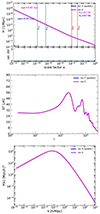 |
Fig. A.1. Model without Λ. The panels display from top to bottom the expansion history, the CMB temperature spectrum and the matter power spectrum of a model universe, which omits Λ but increases the CDM component accordingly, such that the total of the energy densities is equal to the critical density (i.e., a case close to the Einstein-de-Sitter model). The blue curves depict the results obtained by the public version of CLASS. The magenta curves show the results from our amended version, which uses the ICs of the concordance model. The results of both computations agree very well (the magenta curves lie on top of the blue curves). |
For both exotic models, the initial densities are not much different, because we changed the matter components and/or ΩΛ that are subdominant in the early Universe. Therefore, we get basically the same results for both codes.
However, once we picked a case where the ICs were greatly affected, we see a difference, which is illustrated by the following model displayed in Fig. A.2. Here, we omitted Λ (as in the case of Figure A.1), but additionally we reduced the density parameter for radiation by half, compared to its standard value, while increasing the density parameter for the CDM component accordingly. Since radiation is the dominant component in the early Universe, such an extreme change affects the ICs critically (top panel of Fig. A.2). Now, we can see a clear difference between the results from the public and the amended CLASS code in the expansion history, as well as in the spectra. Also, matter-radiation equality aeq and recombination arec are shifted to a later cosmic time, and the present-day expansion rate of H0 = 95.54 km/sec/Mpc, is much higher compared to the configured value of H0 = 67.56 km/sec/Mpc.
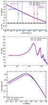 |
Fig. A.2. Model without Λ and less radiation. The panels display from top to bottom the expansion history, the CMB temperature spectrum and the matter power spectrum of a model universe without Λ, whose density parameter for radiation is reduced to half its value of the concordance model, while its CDM density parameter has been accordingly increased, such that the total of the energy densities is equal to the critical density. The blue curves depict the results obtained by the public version of CLASS. The magenta curves show the results from the amended version, which uses the ICs of the concordance model. The results of both computations significantly deviate from each other. |
Of course, the adoption of the concordance EDs, while modifying the density parameter for the radiation component is not in agreement with observations, for both versions of the code. Obviously, this is not a viable procedure in the computation of cosmological models, because it breaks the connection between the EDs and H0 established by the concordance model, as already discussed. In fact, the importance of adopting (keeping) the standard value for the radiation density parameter, especially by excluding it from MCMC parameter space searches, has been known and is handled that way by observational campaigns which apply the standard scheme, see for example, Abbott et al. (2022a) and Alam et al. (2021). To summarize, provided the density parameter of radiation is the same as in the standard, concordance model, the variation of the remaining parameters leads to the same results for both computational procedures, for both the public CLASS code and our amended CLASS code.
Appendix B: Consistency check for ΛCDM
We tested our amended CLASS code by computing observables for the ΛCDM model, and compared them with the results of the original, public version of CLASS. Our amended code used the CPL parametrization, by setting w0 = −1 and wa = 0 in order to recover a cosmological constant. We computed two versions, one based on the parametrization which used the early CMB-based value of H0 from Planck Collaboration VI (2020) (left-hand panels), and another one based on the parametrization which used the local value of H0 from Riess et al. (2022) (right-hand panels). The results and comparison for the expansion histories, as well as for the CMB temperature spectra and matter power spectra, can be found in Fig. B.1.
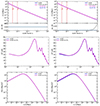 |
Fig. B.1. ΛCDM consistency check. We use our amended version of CLASS to compute observables of the ΛCDM model, using the CPL parametrization with associated parameters w0 = −1 and wa = 0. Left-hand panels: calculation based on the parametrization which uses the early CMB-based value of H0 = 67.56 km/sec/Mpc from Planck Collaboration VI (2020). Since this is equivalent to the standard input in CLASS for ΛCDM, we see no difference in the results. Right-hand panels: calculation based on the parametrization which uses the local value of H0 = 73.04 km/sec/Mpc from Riess et al. (2022). The top row displays the expansion histories, while the middle and bottom rows display the CMB temperature spectra and matter power spectra, respectively. See main text for explanations. |
The left-hand panels show no difference in the results, which is expected, since we parameterize the model in a way that is equal to the standard CLASS input for the concordance ΛCDM model. On the other hand, the right-hand panels show a difference: the expansion history displays similar deviations from the ΛCDM model to those shown in Fig. 9. But the maximum deviation happens at a scale factor of a = 1, in contrast to Fig. 9, where the maximum deviation is at a scale factor of a ∼ 0.8. There are also some minor deviations in the spectra in the right-hand panels, limited to large spatial scales. Assuming that the Hubble tension problem is real, we can recognize that ΛCDM suffers this problem, for the backward and forward evolutions do not yield consistent results. In other words, we see differences in the expansion history (gray curve) from the concordance model when we adopt a locally determined H0 in our model, see right-hand top panel. In this sense, ΛCDM does not pass the recommended consistency check for cosmological models and their parameters, respectively. Thus, there remains a Hubble tension problem in ΛCDM.
All Figures
|
Fig. 1. Evolution of energy densities and expansion rate in the ΛCDM concordance model. Top panel: evolution of the energy densities, determined by Eq. (4). Bottom panel: evolution of the expansion rate H in natural units, determined by the total of the energy densities given by Eq. (5). The vertical lines in blue bracket the epoch of big bang nucleosynthesis, between neutron-proton freeze-out at an/p ∼ 1.3 × 10⁻¹⁰ and nuclei production anuc ∼ 3.3 × 10⁻⁹, while the vertical lines in red (at larger scale factor) indicate the time of matter-radiation equality aeq, followed by recombination arec, in terms of the scale factor a. |
| In the text | |
|
Fig. 2. Illustrative comparison between the evolution of energy density for a component with a constant or nonconstant EoS (arbitrary scaling). The blue component has a constant EoS parameter w = −0.8. The green component has a nonconstant EoS parameter w, which starts out with w = −0.8 (equal to the blue component) and evolves in two steps (indicated by the black vertical solid lines) to w = −0.9 (the slope is indicated by the dashed orange line) and finally to w = −1 (the slope is indicated by the dashed red line). The final density at the present time is higher for the green component. |
| In the text | |
|
Fig. 3. Illustrative evolution of energy densities of components, each with constant EoS (arbitrary scaling). w = −0.8 (blue), w = −0.9 (orange), and w = −1 (red). |
| In the text | |
|
Fig. 4. Illustration of integration orders in determining energy densities of cosmic components. The actual ICs are fixed by processes in the very early Universe, but we have only access to observables at specific later times (respective redshifts or scale factors). The values of the latter determine the value of H, and by extrapolation to the present the value of H0. If H0 determined by the CMB is used, it is this starting point (referred to as “CMB measurement”) which must be used in the integration of Eq. (3): values for the energy densities before this point in time have to be calculated using backward integration, while values for the energy densities after this point in time have to be calculated using forward integration. The green component has a time-dependent w, while the blue component has a constant w = −0.8. |
| In the text | |
|
Fig. 5. Integration with wrong ICs. This illustration complements the one depicted in Fig. 4. The customary backward integration (blue dashed) of the green component with time-dependent EoS parameter leads to incorrect ICs, when we start from the value of H0 determined from observations of the early Universe. |
| In the text | |
|
Fig. 6. Integration with correct ICs. This illustration complements the one depicted in Fig. 4. The customary backward integration of the green component with time-dependent EoS parameter “ends up” at the correct ICs, when we start from the value of H0 determined from observations of the local Universe. |
| In the text | |
|
Fig. 7. CPL models (magenta) and ΛCDM (blue) both computed with the standard procedure. The left-hand side displays the results of the DES-Y3 CPL model with w0 = −0.95 and wa = −0.4. The right-hand side displays the results for the CPL model with w0 = −0.9 and wa = +0.1. We use the original version of CLASS and the value of H0, determined by CMB observations from Planck Collaboration VI (2020). The top panels display the expansion histories, where the vertical lines in red indicate the time of matter-radiation equality at scale factor aeq, followed by recombination arec (both determined by the cosmological model). The bottom insets show the relative deviation of the respective expansion histories (gray curve), which only matters at late times (respective high scale factors). The middle and bottom panels show the CMB temperature spectra (temperature anisotropies) as a function of mode number l, and the matter power spectra as a function of wave number k, respectively. |
| In the text | |
|
Fig. 8. DE component with increasing w: the DES-Y3 CPL model with w0 = −0.95 and wa = −0.4 (magenta) compared to ΛCDM (blue), both computed with our scheme. Panels on the left-hand column were computed using the early parametrization of H0 = 67.56 km s−1 Mpc−1 using Planck Collaboration VI (2020), while panels on the right-hand column employ the local parametrization of H0 = 73.04 km s−1 Mpc−1 from Riess et al. (2022). Top panels: expansion histories; for the vertical lines in red see Fig. 7. We note the deviations in the expansion histories from ΛCDM at late times (respective high scale factors) and the different run of these deviations (see gray curves in the bottom insets of the top panels). Middle panels: CMB temperature spectra. Bottom panels: matter power spectra. The results based on the CMB-determined H0, shown in the left-hand column, display a clear deviation from ΛCDM, whereas the results based on the locally determined H0 are in better agreement with ΛCDM. |
| In the text | |
|
Fig. 9. DE component with decreasing w: a CPL model with w0 = −0.9 and wa = +0.1 (magenta) compared to ΛCDM (blue), both computed with our scheme. Panels on the left-hand column were computed using the early parametrization of H0 = 67.56 km s−1 Mpc−1 from Planck Collaboration VI (2020), while panels on the right-hand column employ the local parametrization of H0 = 73.04 km s−1 Mpc−1 from Riess et al. (2022). Top row: expansion histories; for the vertical lines in red see Fig. 7. Middle panels: CMB temperature spectra. Bottom panels: matter power spectra. In both columns, we see good overall agreement with ΛCDM, except for the fact that the chosen CPL model may provide a resolution to the Hubble tension problem. A difference remains in the present-day Hubble constant between left-hand and right-hand columns, see main text. |
| In the text | |
|
Fig. A.1. Model without Λ. The panels display from top to bottom the expansion history, the CMB temperature spectrum and the matter power spectrum of a model universe, which omits Λ but increases the CDM component accordingly, such that the total of the energy densities is equal to the critical density (i.e., a case close to the Einstein-de-Sitter model). The blue curves depict the results obtained by the public version of CLASS. The magenta curves show the results from our amended version, which uses the ICs of the concordance model. The results of both computations agree very well (the magenta curves lie on top of the blue curves). |
| In the text | |
|
Fig. A.2. Model without Λ and less radiation. The panels display from top to bottom the expansion history, the CMB temperature spectrum and the matter power spectrum of a model universe without Λ, whose density parameter for radiation is reduced to half its value of the concordance model, while its CDM density parameter has been accordingly increased, such that the total of the energy densities is equal to the critical density. The blue curves depict the results obtained by the public version of CLASS. The magenta curves show the results from the amended version, which uses the ICs of the concordance model. The results of both computations significantly deviate from each other. |
| In the text | |
|
Fig. B.1. ΛCDM consistency check. We use our amended version of CLASS to compute observables of the ΛCDM model, using the CPL parametrization with associated parameters w0 = −1 and wa = 0. Left-hand panels: calculation based on the parametrization which uses the early CMB-based value of H0 = 67.56 km/sec/Mpc from Planck Collaboration VI (2020). Since this is equivalent to the standard input in CLASS for ΛCDM, we see no difference in the results. Right-hand panels: calculation based on the parametrization which uses the local value of H0 = 73.04 km/sec/Mpc from Riess et al. (2022). The top row displays the expansion histories, while the middle and bottom rows display the CMB temperature spectra and matter power spectra, respectively. See main text for explanations. |
| In the text | |
Current usage metrics show cumulative count of Article Views (full-text article views including HTML views, PDF and ePub downloads, according to the available data) and Abstracts Views on Vision4Press platform.
Data correspond to usage on the plateform after 2015. The current usage metrics is available 48-96 hours after online publication and is updated daily on week days.
Initial download of the metrics may take a while.