| Issue |
A&A
Volume 683, March 2024
|
|
|---|---|---|
| Article Number | A157 | |
| Number of page(s) | 9 | |
| Section | Extragalactic astronomy | |
| DOI | https://doi.org/10.1051/0004-6361/202348001 | |
| Published online | 15 March 2024 | |
Absence of radio-bright dominance in a near-infrared selected sample of red quasars⋆
1
Cosmic Dawn Center (DAWN), Copenhagen N, Denmark
2
Niels Bohr Institute, University of Copenhagen, Jagtvej 155, 2200 Copenhagen N, Denmark
e-mail: simone.vejlgaard@nbi.ku.dk
3
Centre de Recherche Astrophysique de Lyon, Univ. Claude Bernard Lyon 1, 9 Av. Charles André, 69230 St-Genis-Laval, France
4
European Southern Observatory, Karl-Schwarzschild-Straße 2, 85748 Garching bei München, Germany
5
Instituto de Astrofísica de Canarias, Vía Láctea s/n, 38205 La Laguna, Tenerife, Spain
6
Gran Telescopio Canarias (GRANTECAN), Cuesta de San José s/n, 38712 Breña Baja, La Palma, Spain
Received:
18
September
2023
Accepted:
4
December
2023
Context. The dichotomy between red and blue quasars is still an open question. It is debated whether red quasars are simply blue quasars that are observed at certain inclination angles or if they provide insight into a transitional phase in the evolution of quasars.
Aims. We investigate the relation between quasar colors and radio-detected fraction because radio observations of quasars provide a powerful tool in distinguishing between quasar models.
Methods. We present the eHAQ+GAIA23 sample, which contains quasars from the High A(V) Quasar (HAQ) Survey, the Extended High A(V) Quasar (eHAQ) Survey, and the Gaia quasar survey. All quasars in this sample have been found using a near-infrared color selection of target candidates that have otherwise been missed by the Sloan Digital Sky Survey (SDSS). We implemented a redshift-dependent color cut in g* − i* to select red quasars in the sample and divided them into redshift bins, while using a nearest-neighbors algorithm to control for luminosity and redshift differences between our red quasar sample and a selected blue sample from the SDSS. Within each bin, we cross-matched the quasars to the Faint Images of the Radio Sky at Twenty centimeters (FIRST) survey and determined the radio-detection fraction.
Results. For redshifts 0.8 < z ≤ 1.5, the red and blue quasars have a radio-detection fraction of 0.153−0.032+0.037 and 0.132−0.030+0.034, respectively. The red and blue quasars with redshifts 1.5 < z ≤ 2.4 have radio-detection fractions of 0.059−0.016+0.019 and 0.060−0.016+0.019, respectively, and the red and blue quasars with redshifts z > 2.4 have radio-detection fractions of 0.029−0.012+0.017 and 0.058−0.019+0.024, respectively. For the WISE color-selected red quasars, we find a radio-detection fraction of 0.160−0.034+0.038 for redshifts 0.8 < z ≤ 1.5, 0.063−0.017+0.020 for redshifts 1.5 < z ≤ 2.4, and 0.051−0.022+0.030 for redshifts z > 2.4. In other words, we find similar radio-detection fractions for red and blue quasars within < 1σ uncertainty, independent of redshift. This disagrees with what has been found in the literature for red quasars in SDSS. It should be noted that the fraction of broad absorption line (BAL) quasars in red SDSS quasars is about five times lower. BAL quasars have been observed to be more frequently radio quiet than other quasars, therefore the difference in BAL fractions could explain the difference in radio-detection fraction.
Conclusions. The dusty torus of a quasar is transparent to radio emission. When we do not observe a difference between red and blue quasars, it leads us to argue that orientation is the main cause of quasar redness. Moreover, the observed higher proportion of BAL quasars in our dataset relative to the SDSS sample, along with the higher rate of radio detections, indicates an association of the redness of quasars and the inherent BAL fraction within the overall quasar population. This correlation suggests that the redness of quasars is intertwined with the inherent occurrence of BAL quasars within the entire population of quasars. In other words, the question why some quasars appear red or exhibit BAL characteristics might not be isolated; it could be directly related to the overall prevalence of BAL quasars in the quasar population. This finding highlights the need to explore the underlying factors contributing to both the redness and the frequency of BAL quasars, as they appear to be interconnected phenomena.
Key words: galaxies: active / quasars: general / quasars: supermassive black holes / radio continuum: galaxies
Full Table A.1 is available at the CDS via anonymous ftp to cdsarc.cds.unistra.fr (130.79.128.5) or via https://cdsarc.cds.unistra.fr/viz-bin/cat/J/A+A/683/A157
© The Authors 2024
 Open Access article, published by EDP Sciences, under the terms of the Creative Commons Attribution License (https://creativecommons.org/licenses/by/4.0), which permits unrestricted use, distribution, and reproduction in any medium, provided the original work is properly cited.
This article is published in open access under the Subscribe to Open model. Subscribe to A&A to support open access publication.
1. Introduction
Even though the study of quasi-stellar objects (QSOs, or quasars) began more than half a century ago (Schmidt 1963; Greenstein & Schmidt 1964; Sandage 1965), it remains a field in development. With extremely high bolometric luminosities (up to ∼1047 erg s−1; see, e.g., Onken et al. 2022), quasars are not only the most powerful class of active galactic nuclei (AGN), but also some of the most luminous and distant objects known in the observable Universe (Wu et al. 2015; Wang et al. 2021). Quasars are powered by the rapid accretion of matter onto a supermassive black hole (SMBH) with a possible mass ranging up to 1010 M⊙ (see also Rees 1984). According to the unified model for AGN and quasars presented, for instance, by Antonucci (1993) and Urry & Padovani (1995), a dust torus absorbs and reemits photons from the accretion disk with a dependence on the observed viewing angle. In addition to the broad- and narrow-line regions producing the emission lines used to classify the quasar, the unified model also describes quasar outflows. These outflows can take the form of relativistic and collimated radio jets or more extended winds originating from the accretion disk. In a subset of quasars called broad absorption line (BAL) quasars, the strong winds create broad blueshifted absorption lines in the UV part of the quasar spectrum (Foltz et al. 1987; Weymann et al. 1991).
A typical quasar spectrum is characterized by a rest-frame blue or UV power-law continuum on which broad emission lines are superimposed. However, a number of studies have already confirmed the existence of a quasar population with a much redder continuum, which is simply referred to as “red” quasars (Webster et al. 1995; Benn et al. 1998; Warren et al. 2000; Gregg et al. 2002; Hopkins et al. 2004; Glikman et al. 2007; Fynbo et al. 2013). Our understanding of this particular subset of quasars is still far from complete. While many studies attribute the red optical and infrared (IR) colors to dust obscuration (Sanders et al. 1988a,b), other plausible explanations include starlight contamination from the quasar host galaxy (Serjeant 1996) and differences in the accretion rates (Young et al. 2008). From the attempts to explain the observational differences, two main quasar redness paradigms have emerged: the orientation model, and the evolutionary model. The orientation model claims that any observed differences between red and blue quasars are due to the observer’s viewing angle with respect to the dusty torus, such that inclinations closer to the equatorial plane of the torus correspond to a redder quasar classification (Antonucci 1993). According to the orientation model, the differentiation between red and blue quasars is thus not grounded in physical circumstance, but solely a consequence of relative positioning with respect to either of these objects. The evolutionary model claims that an intrinsic physical evolution is the origin of the quasar redness, such that the red quasar population represents a transitional phase between an early highly dust-obscured star-forming stage and the blue quasar stage (Sanders et al. 1988a,b; Hopkins et al. 2006, 2008; Alexander & Hickox 2012; Glikman et al. 2012). Within this framework, the host galaxies of red quasars are thought to have undergone a major galaxy merger, which induces either strong winds or jets in the central red quasar, with the ability to dissolve their surrounding dust cocoons. This quenches the host galaxy star formation, and the underlying unobscured blue quasar is revealed.
The fact that the optical colors of dust-reddened quasars resemble those of low-mass stars (Richards et al. 2002, 2003) motivated the use of radio selection to build red quasar samples without stellar contamination (Webster et al. 1995; White et al. 2003). Based on their findings, Webster et al. (1995) and White et al. (2003) suggested that up to ∼80% of the total quasar population could be made up of red quasars that were missed by previous optical selection methods. To investigate whether large numbers of dust obscured quasars are indeed missed, Glikman et al. (2007) combined the VLA Faint Images of the Radio Sky at Twenty centimeters (FIRST; Becker et al. 1995) radio survey and the 2 Micron All Sky Survey (2MASS; Skrutskie et al. 2006) in an attempt to counteract the dust bias. However, this introduced a bias toward the radio-bright red quasar population, as pointed out, for example, by Heintz et al. (2016) and Glikman et al. (2018). Combining the Wide-Field Infrared Space Explorer (WISE; Wright et al. 2010) with the Sloan Digital Sky Survey (SDSS; York et al. 2000) and its extension from the Baryon Oscillation Spectroscopic Survey (BOSS; Dawson et al. 2013), Glikman et al. (2022) found it more likely that the red quasars comprise ∼40% of the total quasar population.
Using the SDSS DR7 quasar catalog (Shen et al. 2011), Klindt et al. (2019) investigated the fundamental differences between red and blue quasars seen in radio wavelengths. Searching for mid-IR (MIR) counterparts and checking for luminosity and redshift effects, they cross-matched the SDSS DR7 quasar catalog with sources in the FIRST survey and found a fraction of the radio detection among the red quasars that was about a factor of 3 higher than that of the blue quasars. Klindt et al. (2019) claimed that this provided evidence against the orientation-dependent model because radio emission is not affected by dust, and hence, orientation alone cannot explain the observed differences. In a follow-up study, Fawcett et al. (2020) found that the radio excess decreased toward the radio-quiet part of the red quasar population, but concluded that the excess is still significant. Furthermore, Fawcett et al. (2023) found an intrinsic relation between dust reddening and the production of radio emission in quasars when studying MIR and optical-color selected quasars in the Dark Energy Spectroscopic Instrument (DESI) survey. This relation is such that low-powered jets, winds, or outflows are thought to cause shocks in the dusty quasar environment, which then powers radio emission. However, clues pointing toward a lack of radio detection excess have also been presented previously (see, e.g., Krogager et al. 2016a). When Krogager et al. (2016a) compared their red quasar radio detection fraction to the radio detection fraction of the red quasars overlapping in SDSS+BOSS, the overlapping quasars showed a significantly higher radio detection fraction, which demonstrates that the radio excess might be a selection artifact.
In this paper, we examine the entire sample of quasars found by Fynbo et al. (2013), Krogager et al. (2015, 2016a), and Heintz et al. (2020). This sample contains quasars that have been missed by classic quasar selection methods, such as those used to build the SDSS DR7 quasar catalog. Fynbo et al. (2013) showed that these quasars differ from the classically selected quasars by an increased dust reddening. Furthermore, the dust-reddening was not found to be caused by intervening absorbers, but was instead shown to be primarily a consequence of the quasar host galaxy. In Sect. 2, we outline how we gathered the sample, and in Sect. 3, we describe how we ensured that color was the only observed difference between our red quasar sample and the blue SDSS DR7 quasars with which we compared our sample. We present the results of our investigation in Sect. 4. Throughout Sect. 4, we also compare our results to the blue SDSS DR7 quasars in order to search for fundamental differences between red and blue quasars. The comparison of our results to the orientation and evolution model is presented in Sect. 5, where we also discuss the other parameters that might influence our findings. Following the Planck Collaboration VI (2020), we assume a flat ΛCDM cosmology with H0 = 67.4 km s−1 Mpc−1, ΩΛ = 0.685, and ΩM = 0.315 throughout the paper. We use Vega magnitudes throughout the paper, except for Sect. 3.3, where we convert into AB magnitudes to calculate the rest-frame 6 μm luminosity.
2. Sample
We built our sample of quasars from the catalog of quasar candidates provided in Fynbo et al. (2013, hereafter F13), Krogager et al. (2015, hereafter K15), Krogager et al. (2016a, hereafter K16) and Heintz et al. (2020, hereafter H20). For each candidate, we have broadband photometry from the u (3543 Å), g (4770 Å), r (6231 Å), i (7625 Å), and z (9134 Å) bands from SDSS and the J, H, K bands from UKIRT Infrared Deep Sky Survey (UKIDSS; Lawrence et al. 2007). UKIDSS uses the Wide Field Camera (WFCAM) on the 3.8 m United Kingdom Infra-red Telescope (UKIRT). In some cases (∼10% of the objects), the NIR band was instead taken from the VISTA (Emerson et al. 2006; Dalton et al. 2006) Kilo-degree Infrared Galaxy (VIKING; Edge et al. 2013) survey. The candidates from F13 all have 0.8 < g* − r* < 1.5 and r* − i* > 0.2, while the candidates from K15 and K16 have 0.5 < g* − r* < 1.0 and g* − r* > 0.5, respectively. H20 have relied purely on an astrometric selection of quasars as stationary sources in the Gaia survey.
The sample also contains quasars that have not been published previously, and a few that have been published in single-object studies (Fynbo et al. 2017, 2020; Heintz et al. 2018; Geier et al. 2019). These quasars were selected with a combination of optical colors as in K16 and astrometric exclusion of stellar sources as in H20. We refer to Heintz et al. (2018) and Geier et al. (2019) for further details on the selection of these quasars. The unpublished parts of the survey make up ∼50% of the total survey.
None of the papers claim to provide an unbiased selection method. On the contrary, they specifically searched for reddened quasars with the main motivation of finding foreground dusty damped Lyman-α absorbers (DLAs). Radio emission has not been part of the selection criteria for any of the quasar candidates. It should also be noted that the quasars were selected specifically to not appear in SDSS spectroscopic database. In total, 550 of the 578 quasar candidates turned out to be quasars after follow-up spectroscopy.
In order for the quasars to be included in our sample, we also introduced the requirement of a spectroscopic redshift. These redshifts are obtained as part of dedicated spectroscopic observations with visually inspected redshift determinations for all objects. We refer to the list of references for the surveys in the appendix for further details. Five hundred and forty-three of the total 550 quasars fulfill this requirement. In addition to the broadband photometric data and spectroscopic redshifts, we also searched for MIR counterparts of the quasars using WISE (Wright et al. 2010) and radio counterparts using FIRST (Becker et al. 1995, 2012; Helfand et al. 2015). FIRST operates at a frequency of 1.4 GHz (20 cm wavelength) and offers a high sensitivity of typically about 1 mJy for point sources. With an angular resolution as fine as 5 arcsec, FIRST covers over 10 000 deg2 of the northern sky in a region that is largely coincident with SDSS. For the detections, we adopted a 10 arcsec cross-matching radius. We took the closest-distance match within the 10 arcsec to be the radio counterpart. It should be noted that the largest match distance we found is 1.2 arcsec. In the case of multiple sources within the 10 arcsec search radius, we also checked SDSS for the existence of multiple optical sources. This was only the case for one of the quasars: CQ0155+0438. Hence, we did not include CQ0155+0438 in the sample. We find that 534 of the redshift-confirmed quasars have MIR counterparts, while a small subset of 33 quasars have radio counterparts detected in FIRST. We consider the 534 MIR counterpart quasars to be the parent sample for our study here and call this sample the eHAQ+GAIA23 sample. We chose this name because the sample contains sources from the HAQ Survey, the eHAQ Survey, and the Gaia quasar survey. The number 23 represents the year 2023, in which this project was carried out. See the appendix for details on accessing the published data.
3. Methods
In order to facilitate a direct comparison to the blue SDSS DR7 quasars, we followed the method in Klindt et al. (2019). Their method consists of two steps taken to reduce the differences that are not related to color between the red and blue SDSS DR7 quasar population. First, they used g* − i* color quantile cuts to define a red and a blue quasar population. Then, they used an unsupervised nearest-neighbor algorithm in the rest-frame 6 μm luminosity-redshift space to match every red quasar with a blue one. These steps are performed to ensure that the populations are similar in all other parameters apart from color, which means that any differences can be attributed to the color of the quasars. Redshift and 6 μm luminosity are chosen above other dependences because they have a potentially high impact on the quasar color. When we do not take redshift into account, a high-redshift blue quasar might seem red. The 6 μm rest-frame luminosity is a measure of the thermal emission from warm–hot dust in the quasar torus. It is heated by the accretion disk emission and indicates the central black hole accretion level, which is correlated to the bolometric luminosity of the quasar (Hickox & Alexander 2018). By matching this luminosity distribution for the two different color populations, we ensure that the quasar activity levels are similar.
3.1. Redshift dependence
One of the keystones in exploring the differences between red and blue quasars is to ensure that the only observed difference in the sample is the color. To do this, we applied several cuts on the sample redshift. We divided the eHAQ+GAIA23 sample into two redshift bins: z1, including quasars with 0.8 < z ≤ 1.5, and z2, including those with 1.5 < z ≤ 2.4. However, we also decided to study z3, including those with 2.4 < z ≤ 4.25. The resulting number of quasars within each redshift bin is presented in Table 1.
Number of quasars in the eHAQ+GAIA23 catalog.
3.2. Color dependence
We also ensured that we defined a red and a blue quasar in the same manner as Klindt et al. (2019). They defined a red quasar as a quasar with a g* − i* color value in the upper 10th percentile of the SDSS DR7 quasar catalog g* − i* color values, while a blue quasar should belong to the lower 10th percentile of the SDSS DR7 QC g* − i* color values. All quasars in between these percentiles are defined as not-red control quasars. Klindt et al. (2019) already noted that this might lead to issues in the z3 bin, where the g* band is affected by the Lyman-α break. For this reason, we conducted our analysis with and without the z3 bin. In Fig. 1, we show the color selection as a black line on top of the g* − i* color versus redshift distribution of each quasar in the eHAQ+GAIA23 sample. The number of red quasars (rQSO) and red quasars with a radio detection (FrQSO) can be found in Table 1. It is evident from this table that 423 of the eHAQ+GAIA23 quasars are red, and the remaining 111 are not red. Upon inspecting the distribution of these two quasar classes across the three redshift bins, we observe that the red quasars are predominantly concentrated in the middle redshift bin, where ∼40% of them are found. The not-red quasars in eHAQ+GAIA23 are primarily located in the highest redshift bin, where ∼80% of them are found. One explanation for this could be that SDSS contains a smaller fraction of red quasars at higher redshifts, and hence the quantile cut is pushed toward higher g* − i* values.
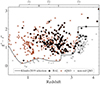 |
Fig. 1. Distribution of the g* − i* color as a function of redshift for the quasars in the new quasar catalog. Every cross represents a quasar. The black line shows the red quasar selection criteria from Klindt et al. (2019), such that quasars with a higher color value are labeled rQSO and are shown in red in this figure, while those with a lower color value are labeled not-red QSO and are shown in gray in this figure. The categorization of the BAL quasars, marked with black circles, relied on visual assessment without the application of rigid standards (see F13, K15, K16, H20). |
As can be seen from Table 1, 179 of the eHAQ+GAIA23 quasars qualify as BAL, meaning that this new catalog contains ∼34% BAL quasars. For the red quasars alone, we find 163 red BAL quasars out of 423 red quasars. For the red quasars, the BAL percentage therefore increases to ∼39% BAL quasars. For comparison, we include the BAL number statistics from the SDSS DR7 quasar catalog (Shen et al. 2011) in Table 2.
Statistics of the quasar distribution with respect to the number of BALs.
3.3. Luminosity dependence
To ensure that any difference between the red and blue quasars cannot be explained by differences in the rest-frame luminosities, we determined the rest-frame 6 μm luminosity of the red quasars in our sample and compared them to the rest-frame 6 μm luminosities of the red and blue SDSS quasars. We used the MIR-magnitude data from WISE. First, we converted from the WISE Vega-system into AB magnitudes using mAB = mVega + Δm, where Δm = 3.339 for the W2 band and Δm = 5.174 for the W3 band (Tokunaga & Vacca 2005). Under the assumption that the magnitudes are monochromatic at the effective filter wavelength, we converted from AB magnitudes into flux densities following the definition given by Tokunaga & Vacca (2005). We performed a log-linear fit between the W2 and W3 effective filter wavelength flux densities, which we used to either interpolate or extrapolate the rest-frame 6 μm flux density, depending on the quasar redshift. It should be noted that for the highest-redshift quasar, we extrapolated up to ∼30 μm. At this wavelength, the extrapolation is not necessarily reliable. The rest-frame 6 μm luminosity L6 μm distribution as a function of redshift is shown in Fig. 2a.
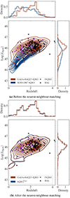 |
Fig. 2. Luminosity vs. redshift distribution. The red kernel density estimate plot represents the red eHAQ+GAIA23 quasar distribution, and each purple dot represents a radio-detected red quasar. The black circles represent red BAL quasars. In addition to these markers, the blue kernel density estimate plot shows the blue SDSS DR7 quasars. Center: logarithm of the rest-frame 6 μm luminosity of either all the blue SDSS quasars (a) or the redshift–luminosity matched blue SDSS quasars (b) in blue curves and the red eHAQ+GAIA23 quasars in red curves as a function of redshift, assuming a continuous probability density curve. Top: density histogram of the redshift for the two different populations. Right: density histogram of the rest-frame 6 μm luminosity for the two different populations. |
With respect to ensuring that the only observed difference between our red quasars and the SDSS blue quasars is the color, we need to correct this difference in the luminosity distributions. Without any form of correction, the difference prohibits us from excluding that any other difference observed between the two populations is more than the mere result of a correlation with the rest-frame 6 μm luminosity.
Even though the redshift distributions of the blue SDSS population and the red eHAQ+GAIA23 population look similar, the top histogram in Fig. 2a shows a shift toward higher redshifts for our red quasars. The right histogram in Fig. 2b reveals a clear difference in the two luminosity distributions. While the red eHAQ+GAIA23 quasar sample has a luminosity median of  , the blue SDSS population has a lower and visibly broader luminosity distribution with median
  . In order to remove this difference and be able to report differences related solely to quasar color, we followed an approach similar to the one taken by Klindt et al. (2019): We ran the red eHAQ+GAIA23 quasars through a scikit-learn (Pedregosa et al. 2011), unsupervised nearest-neighbor algorithm in the rest-frame 6 μm luminosity–redshift space. For each of our red sample quasars, the algorithm found an SDSS blue quasar within a fixed tolerance of 0.1 dex in luminosity space and 0.1 in redshift space. After using the nearest-neighbor algorithm, the redshift–luminosity matched blue quasars show a rest-frame 6 μm luminosity distribution with median
  .
.
Figure 2b shows the kernel density estimate plot after using the nearest-neighbor algorithm. This served mainly as a sanity check and revealed that the approach has the intended effect. The redshift–luminosity matched blue quasars show a rest-frame 6 μm luminosity distribution with median  .
.
3.4. Host galaxy dependence
In Fig. 3, the distribution of the red quasars in the eHAQ+GAIA23 sample is shown in the W2 − W3 vs. W1 − W2 color space alongside the AGN wedge from Mateos et al. (2012). Each cross represents a red quasar, while the color of the cross is determined by the quasar redshift. The dots show the distribution of the red quasars with radio detection, and a black circle marks which of the red quasars are BAL quasars. Table 3 shows that 59 of the 423 red quasars lie outside the AGN wedge. The highest percentage is found in the z > 2.4 sample. Even though the AGN torus is expected to dominate the emission at MIR wavelengths, emission from star formation in the host galaxy might still contaminate the spectrum. If the MIR fluxes are indeed contaminated by the host galaxy, this would bias our rest-frame 6 μm luminosity calculations. The AGN wedge systematically deselects spectra for which the host galaxy star-formation contributes more than 10% to the MIR luminosity emitted by the AGN. Spectra with a contamination from star formation luminosity > 10% end on the lower right side of the wedge (Mateos et al. 2012). This explains that the highest percentage of quasars outside the AGN wedge is found in the highest-redshift sample, which is a more active part of the star formation history (Madau & Dickinson 2014). The red BAL quasars show a similar pattern, with an outside percentage peaking at z3. Only the small subcategory of red quasars with a radio detection have no outliers with respect to the AGN wedge.
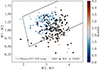 |
Fig. 3. Red quasar distribution in the WISE (W2 − W3,W1 − W2) color space. Each cross is a red quasar, each dot is a radio quasar, and each black circle indicates whether the red quasar is a BAL quasar. The color of the markers depends on the quasar redshifts. |
Statistics of the red and redshift–luminosity matched blue quasar distribution with respect to the AGN wedge in WISE colors as defined by Mateos et al. (2012).
The statistics presented in Table 3 generally have a higher number of quasars outside the AGN wedge compared to the SDSS population of blue quasars, but not compared to the redshift–luminosity matched subpopulation. The redshift–luminosity matched subpopulation has a higher percentage of quasars outside the AGN wedge at redshifts z > 1.5. The comparison between red and blue quasars was to be as unaffected by other physical parameters as possible. Therefore, we proceeded to run the unsupervised nearest-neighbor algorithm on the red quasars within the AGN wedge and drew neighbors from the full blue SDSS quasar population. This yielded a rest-frame 6 μm luminosity distribution with median  . This is similar to what we found when we included quasars outside the AGN wedge.
4. Results: Radio-detection rates
In Table 4, we report the FIRST-detected percentage in each of the three redshifts bins for the two different subsamples of red eHAQ+GAIA23 quasars described in Sects. 3.2 and 3.4. We also report the FIRST-detected percentage for the luminosity–redshift matched SDSS sample of blue quasars described in Sect. 3.3. All values were calculated using the Bayesian binomial confidence interval (CI) method described in Cameron (2011), such that the reported value is the 50% CI and the lower and upper uncertainty are the 15.87% and 84.13% CI (±1σ), respectively. The leftmost column displays the FIRST-detected percentage of the red quasars (rQSO) selected as described in Sect. 3.2, while the center column displays the FIRST-detected percentage of the red quasars within the AGN wedge (AGN-w rQSO). As shown in Fig. 2a, these percentages should not be compared directly to the blue quasar FIRST-detected percentages reported by Klindt et al. (2019) because of the differences in the rest-frame 6 μm luminosity distributions. Instead, we report the FIRST-detected percentage of the redshift–luminosity matched blue quasar population in the rightmost column of Table 4.
FIRST-detected percentage in each of the redshift bins for two subsamples of the new catalog: the red quasars (rQSO), and the red quasars within the AGN wedge (AGN-w rQSO).
The values reported in Table 4 are plotted in Fig. 4. In this figure, the dark red dots with error bars represent the fraction of FIRST-detected red quasars and their 1σ upper and lower limits. The orange diamonds and error bars represent the fraction of FIRST-detected red quasars with observed colors within the AGN wedge and their limits. The area shown by the blue hashed region highlight the area corresponding to the fraction of FIRST-detected redshift–luminosity matched blue SDSS quasars ±1σ errors. Similarly, the shaded purple region highlight the area corresponding to the fraction of FIRST-detected blue SDSS quasars matched with redshift–luminosity to our red quasars within the AGN wedge.
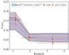 |
Fig. 4. FIRST-detected fraction as a function of redshift for the two different subsamples of our new catalog: The red quasars (rQSO) shown in dark red, and the red quasars within the AGN wedge (AGN-w rQSO) shown in orange. The luminosity–redshift matched blue quasars from SDSS are also included. The area highlighted by blue diagonal stripes corresponds to their detection fraction ±1σ confidence intervals. The shaded purple area highlights the area corresponding to the blue SDSS quasars matched with redshift–luminosity to our red quasars within the AGN wedge. The two dashed lines show the median of the luminosity–redshift matched blue quasars from SDSS and the blue SDSS quasars matched with redshift–luminosity to our red quasars within the AGN wedge. |
Figure 4 illustrates that the red quasars in the eHAQ+GAIA23 sample do not show a higher radio detection rate within 1σ than the blue quasar sample for any redshifts. Even when we exclude the red quasars outside the AGN wedge, the detection fraction of radio emission is the same within the 1σ confidence intervals compared to the blue quasar sample in all redshift bins. Even though it is not statistically significant, we note that the red quasar values are at the top part of the blue quasar distribution in the lowest-redshift bin. In the highest-redshift bin, the red quasar values lie in the lower part of the blue quasar distribution, even though this is not statistically significant either.
5. Discussion and conclusions
We have presented an analysis of the radio-detection fraction of the red quasars in eHAQ+GAIA23. Using a color-cut criterion in the g* − i* color space, we selected only quasars that would belong to the upper 10th g* − i* color percentile of quasars in the SDSS quasar catalog. Neither of the redshift bins show an excess of sources with radio emission detected in FIRST compared to redshift–luminosity matched SDSS blue quasars.
5.1. Quasar redness models
Orientation-dependent models claim that the redness of quasars can be explained by the viewing angle with respect to the dusty torus (Antonucci 1993; Urry & Padovani 1995; Netzer 2015). In this framework, red quasars are simply observed with an inclination angle and hence through the dusty torus, while blue quasars are observed face-on. While the intervening dusty torus will change the optical colors, the radio emission remains unaffected. Under the assumption that the dusty torus is the only cause of the observed redness, there should thus be no difference in the radio emission from red and blue quasars. In this manner, our findings support the orientation model for quasar redness.
On the other hand, the evolutionary models attribute the redness of quasars to different phases in the life of quasars. A red quasar evolves from an early-phase blue quasar that has developed strong winds in order to drive its initial layers of dust and gas away and reveal the hidden accretion disk within. Thus, these models suggest that red quasars have stronger winds than blue quasars. Strong winds have been associated with weak radio emission (Mehdipour & Costantini 2019), which suggests that red quasars should have fewer detected sources at a constant detection sensitivity. This is not what we observe for our sample, and hence our findings only provide evidence for the orientation-dependent model for quasar redness.
5.2. The BAL Effect
The strong winds of the evolutionary model framework are a well-known characteristic of BAL quasars. Following the results of Mehdipour & Costantini (2019), it is expected that BAL quasars are more frequently radio quiet than other quasars. In the context of explaining why the red eHAQ+GAIA23 quasars have a similar radio detection fraction compared to their luminosity–redshift matched blue SDSS quasars, we recall from Table 2 that our red quasar sample has a high BAL fraction even at redshifts z < 2.4. With a higher fraction of radio-quiet quasars, it is expected that the radio-detection fraction decreases. In other words, it is possible that the radio-detection fraction of the red eHAQ+GAIA23 quasars is lower solely because of the higher BAL quasar fraction. This links the question of whether the radio detection fraction depends on quasar color to the question of the intrinsic BAL quasar fraction in the total quasar population. The BAL quasar fraction remains an open question, but the recent study by Bischetti et al. (2023) estimated it to increase with redshift from ∼20% at redshift z ∼ 2 − 4 to ∼50% at redshift z ∼ 6. An exploration of the BAL fraction of the total red quasar population would require a selection cut that is unbiased against BAL and red quasars.
5.3. Selection effects
The quasars in eHAQ+GAIA23 are not selected to be unbiased. Instead, the selection criteria aim to target red quasars, in particular, to explore how frequently quasars are reddened by dusty foreground absorbers at redshifts z ≳ 2 (Krogager et al. 2016b; Geier et al. 2019). Hence, the chosen selection cuts are also expected to play a role in the results presented in this work. The HAQ Survey presented by F13 led the later surveys and particularly the eHAQ Survey to an increased focus on targeting fewer quasars at redshifts z < 2 with high dust reddening as well as fewer unobscured quasars at redshifts z > 3.5. This resulted in a decrease of intrinsically red quasars at lower redshifts, especially at redshifts z ≲ 1.5. One of the main reasons for doing so is to ensure the ability to detect Ly-α in absorption in the observed spectra from the surveys, which had posed a problem for the HAQ Survey (see K16).
Even though the original purpose of the survey was aided by this, the intended bias subtly compromises our results for red quasars with redshifts 0.8 < z ≤ 1.5. In addition to explaining why the combined surveys have fewer quasars in this redshift bin, the focus might also explain why this population behaves more similar to the red SDSS quasars with radio-detection fractions in the upper part of the luminosity–redshift matched blue SDSS quasar distribution.
The DESI survey quasars studied, for example, by Fawcett et al. (2023) also behave more similar to the SDSS quasars. These quasars are selected based on MIR and optical color and display an intrinsic relation between dust reddening and the production of radio emission. In contrast to the eHAQ+GAIA23 quasars, the DESI survey quasars might not be selected completely independently from the SDSS quasars. In addition to color cuts in the MIR and optical colors, Chaussidon et al. (2023) used a random forest machine-learning algorithm to improve the success rate for DESI with respect to quasars. This algorithm is trained on quasars known from the SDSS Stripe 82, which opens the possibility for a correlation between the SDSS and the DESI quasars. Hence, the need for a color-unbiased quasar sample remains.
5.4. Conclusion and future work
Our analysis of the radio-detection fraction of red quasars in the eHAQ+GAIA23 sample, when compared to the SDSS blue quasars, provides significant insights into the nature of quasar redness. Our findings predominantly support the orientation-dependent model, suggesting that the redness of quasars is primarily a result of the viewing angle relative to the dusty torus. This conclusion is drawn from the observation that there is no significant difference in the radio emission between red and blue quasars. This aligns with the expectation that the dusty torus affects optical colors without influencing radio emission. In contrast, the evolutionary model, which links quasar redness to different developmental phases and associates strong winds with weak radio emission, finds less support in our data. The lack of a statistically discernible decrease in radio detection fraction in red quasars, as predicted by the evolutionary model, suggests that the red quasar redness is less likely to be due to this phase-based evolution. Furthermore, the intricacies of our sample selection in eHAQ+GAIA23, with a particular focus on red quasars and the exclusion of certain quasar populations due to survey biases, have implications for our results. While these biases were essential for the previous survey’s objectives, they also limit the generalizability of our conclusions, particularly in the context of the broader quasar population.
In future works, we will analyze the red quasar spectra further to provide more details on the emission and absorption lines of this quasar population. On larger timescales, a hope for a future disentanglement of the selection biases discussed here has been presented with the 4-m Multi-Object Spectroscopic Telescope (4MOST) Gaia purely astrometric quasar survey (4G-PAQS, Krogager et al. 2023). With its wide-field, high-multiplex, optical spectroscopic survey facility (de Jong et al. 2019), 4MOST will provide a unique opportunity to build the first color-unbiased quasar survey based solely on astrometry from Gaia without an assumption on the spectral shape. However, it should be noted that the 4G-PAQS will still be limited in magnitude due to its selection of Gaia-detected sources. The 4G-PAQS community survey will target a total of approximately 300 000 quasar candidates. In addition to studying quasar feedback through BAL outflows at redshifts 0.8 < z < 4, 4G-PAQS will also aim to quantify the dust bias in quasar absorption systems at redshifts 2 < z < 3. This will provide a larger unbiased sample of both red and not-red quasars to determine the origin of the differences between red and blue quasars.
Acknowledgments
The Cosmic Dawn Center (DAWN) is funded by the Danish National Research Foundation under grant DNRF140. SV and JPUF is supported by the Independent Research Fund Denmark (DFF–4090-00079) and thanks the Carlsberg Foundation for support. L.C. and G.M. are supported by the Independent Research Fund Denmark (DFF 2032-00071). K.E.H. acknowledges support from the Carlsberg Foundation Reintegration Fellowship Grant CF21-0103. This publication makes use of data products from the Wide-field Infrared Survey Explorer, which is a joint project of the University of California, Los Angeles, and the Jet Propulsion Laboratory/California Institute of Technology, funded by the National Aeronautics and Space Administration. This publication makes use of data products from the Two Micron All Sky Survey, which is a joint project of the University of Massachusetts and the Infrared Processing and Analysis Center/California Institute of Technology, funded by the National Aeronautics and Space Administration and the National Science Foundation. Funding for SDSS-III has been provided by the Alfred P. Sloan Foundation, the Participating Institutions, the National Science Foundation, and the US Department of Energy Office of Science. The SDSS-III web site is http://www.sdss3.org/. SDSS-III is managed by the Astrophysical Research Consortium for the Participating Institutions of the SDSS-III Collaboration including the University of Arizona, the Brazilian Participation Group, Brookhaven National Laboratory, Carnegie Mellon University, University of Florida, the French Participation Group, the German Participation Group, Harvard University, the Instituto de Astrofisica de Canarias, the Michigan State/Notre Dame/JINA Participation Group, Johns Hopkins University, Lawrence Berkeley National Laboratory, Max Planck Institute for Astrophysics, Max Planck Institute for Extraterrestrial Physics, New Mexico State University, New York University, Ohio State University, Pennsylvania State University, University of Portsmouth, Princeton University, the Spanish Participation Group, University of Tokyo, University of Utah, Vanderbilt University, University of Virginia, University of Washington, and Yale University. When (some of) the data reported here were obtained, UKIRT was supported by NASA and operated under an agreement among the University of Hawaii, the University of Arizona, and Lockheed Martin Advanced Technology Center; operations were enabled through the cooperation of the East Asian Observatory.
References
- Alexander, D. M., & Hickox, R. C. 2012, New Astron. Rev., 56, 93 [Google Scholar]
- Antonucci, R. 1993, ARA&A, 31, 473 [Google Scholar]
- Becker, R. H., White, R. L., & Helfand, D. J. 1995, ApJ, 450, 559 [Google Scholar]
- Becker, R. H., Helfand, D. J., White, R. L., Gregg, M. D., & Laurent-Muehlheisen, S. A. 2012, VizieR Online Data Catalog: VIII/90 [Google Scholar]
- Benn, C. R., Vigotti, M., Carballo, R., Gonzalez-Serrano, J. I., & Sanchez, S. F. 1998, MNRAS, 295, 451 [NASA ADS] [CrossRef] [Google Scholar]
- Bischetti, M., Fiore, F., Feruglio, C., et al. 2023, ApJ, 952, 44 [NASA ADS] [CrossRef] [Google Scholar]
- Cameron, E. 2011, PASA, 28, 128 [Google Scholar]
- Chaussidon, E., Yèche, C., Palanque-Delabrouille, N., et al. 2023, ApJ, 944, 107 [NASA ADS] [CrossRef] [Google Scholar]
- Dalton, G. B., Caldwell, M., Ward, A. K., et al. 2006, in SPIE Conf. Ser., eds. I. S. McLean, & M. Iye, 6269, 62690X [NASA ADS] [Google Scholar]
- Dawson, K. S., Schlegel, D. J., Ahn, C. P., et al. 2013, AJ, 145, 10 [Google Scholar]
- de Jong, R. S., Agertz, O., Berbel, A. A., et al. 2019, The Messenger, 175, 3 [NASA ADS] [Google Scholar]
- Edge, A., Sutherland, W., Kuijken, K., et al. 2013, The Messenger, 154, 32 [NASA ADS] [Google Scholar]
- Emerson, J., McPherson, A., & Sutherland, W. 2006, The Messenger, 126, 41 [NASA ADS] [Google Scholar]
- Fawcett, V. A., Alexander, D. M., Rosario, D. J., et al. 2020, MNRAS, 494, 4802 [Google Scholar]
- Fawcett, V. A., Alexander, D. M., Brodzeller, A., et al. 2023, MNRAS, 525, 5575 [CrossRef] [Google Scholar]
- Foltz, C. B., Weymann, R. J., Morris, S. L., & Turnshek, D. A. 1987, ApJ, 317, 450 [NASA ADS] [CrossRef] [Google Scholar]
- Fynbo, J. P. U., Krogager, J. K., Venemans, B., et al. 2013, ApJS, 204, 6 [NASA ADS] [CrossRef] [Google Scholar]
- Fynbo, J. P. U., Krogager, J. K., Heintz, K. E., et al. 2017, A&A, 606, A13 [NASA ADS] [CrossRef] [EDP Sciences] [Google Scholar]
- Fynbo, J. P. U., Møller, P., Heintz, K. E., et al. 2020, A&A, 634, A111 [NASA ADS] [CrossRef] [EDP Sciences] [Google Scholar]
- Geier, S. J., Heintz, K. E., Fynbo, J. P. U., et al. 2019, A&A, 625, L9 [NASA ADS] [CrossRef] [EDP Sciences] [Google Scholar]
- Glikman, E., Helfand, D. J., White, R. L., et al. 2007, ApJ, 667, 673 [NASA ADS] [CrossRef] [Google Scholar]
- Glikman, E., Urrutia, T., Lacy, M., et al. 2012, ApJ, 757, 51 [Google Scholar]
- Glikman, E., Lacy, M., LaMassa, S., et al. 2018, ApJ, 861, 37 [NASA ADS] [CrossRef] [Google Scholar]
- Glikman, E., Lacy, M., LaMassa, S., et al. 2022, ApJ, 934, 119 [NASA ADS] [CrossRef] [Google Scholar]
- Greenstein, J. L., & Schmidt, M. 1964, ApJ, 140, 1 [NASA ADS] [CrossRef] [Google Scholar]
- Gregg, M. D., Lacy, M., White, R. L., et al. 2002, ApJ, 564, 133 [Google Scholar]
- Heintz, K. E., Fynbo, J. P. U., Møller, P., et al. 2016, A&A, 595, A13 [NASA ADS] [CrossRef] [EDP Sciences] [Google Scholar]
- Heintz, K. E., Fynbo, J. P. U., Ledoux, C., et al. 2018, A&A, 615, A43 [NASA ADS] [CrossRef] [EDP Sciences] [Google Scholar]
- Heintz, K. E., Fynbo, J. P. U., Geier, S. J., et al. 2020, A&A, 644, A17 [NASA ADS] [CrossRef] [EDP Sciences] [Google Scholar]
- Helfand, D. J., White, R. L., & Becker, R. H. 2015, ApJ, 801, 26 [NASA ADS] [CrossRef] [Google Scholar]
- Hickox, R. C., & Alexander, D. M. 2018, ARA&A, 56, 625 [Google Scholar]
- Hopkins, P. F., Strauss, M. A., Hall, P. B., et al. 2004, AJ, 128, 1112 [Google Scholar]
- Hopkins, P. F., Somerville, R. S., Hernquist, L., et al. 2006, ApJ, 652, 864 [NASA ADS] [CrossRef] [Google Scholar]
- Hopkins, P. F., Hernquist, L., Cox, T. J., & Kereš, D. 2008, ApJS, 175, 356 [Google Scholar]
- Klindt, L., Alexander, D. M., Rosario, D. J., Lusso, E., & Fotopoulou, S. 2019, MNRAS, 488, 3109 [Google Scholar]
- Krogager, J. K., Geier, S., Fynbo, J. P. U., et al. 2015, ApJS, 217, 5 [NASA ADS] [CrossRef] [Google Scholar]
- Krogager, J. K., Fynbo, J. P. U., Heintz, K. E., et al. 2016a, ApJ, 832, 49 [CrossRef] [Google Scholar]
- Krogager, J. K., Fynbo, J. P. U., Noterdaeme, P., et al. 2016b, MNRAS, 455, 2698 [NASA ADS] [CrossRef] [Google Scholar]
- Krogager, J. K., Leighly, K. M., Fynbo, J. P. U., et al. 2023, The Messenger, 190, 38 [NASA ADS] [Google Scholar]
- Lawrence, A., Warren, S. J., Almaini, O., et al. 2007, MNRAS, 379, 1599 [Google Scholar]
- Madau, P., & Dickinson, M. 2014, ARA&A, 52, 415 [Google Scholar]
- Mateos, S., Alonso-Herrero, A., Carrera, F. J., et al. 2012, MNRAS, 426, 3271 [Google Scholar]
- Mehdipour, M., & Costantini, E. 2019, A&A, 625, A25 [NASA ADS] [CrossRef] [EDP Sciences] [Google Scholar]
- Netzer, H. 2015, ARA&A, 53, 365 [Google Scholar]
- Onken, C. A., Lai, S., Wolf, C., et al. 2022, PASA, 39, e037 [NASA ADS] [CrossRef] [Google Scholar]
- Pedregosa, F., Varoquaux, G., Gramfort, A., et al. 2011, J. Mach. Learn. Res., 12, 2825 [Google Scholar]
- Planck Collaboration VI. 2020, A&A, 641, A6 [NASA ADS] [CrossRef] [EDP Sciences] [Google Scholar]
- Rees, M. J. 1984, ARA&A, 22, 471 [Google Scholar]
- Richards, G. T., Fan, X., Newberg, H. J., et al. 2002, AJ, 123, 2945 [NASA ADS] [CrossRef] [Google Scholar]
- Richards, G. T., Hall, P. B., Vanden Berk, D. E., et al. 2003, AJ, 126, 1131 [Google Scholar]
- Sandage, A. 1965, ApJ, 141, 1560 [NASA ADS] [CrossRef] [Google Scholar]
- Sanders, D. B., Soifer, B. T., Elias, J. H., et al. 1988a, ApJ, 325, 74 [Google Scholar]
- Sanders, D. B., Soifer, B. T., Elias, J. H., Neugebauer, G., & Matthews, K. 1988b, ApJ, 328, L35 [NASA ADS] [CrossRef] [Google Scholar]
- Schmidt, M. 1963, Nature, 197, 1040 [Google Scholar]
- Serjeant, S. 1996, Nature, 379, 304 [Google Scholar]
- Shen, Y., Richards, G. T., Strauss, M. A., et al. 2011, ApJS, 194, 45 [Google Scholar]
- Skrutskie, M. F., Cutri, R. M., Stiening, R., et al. 2006, AJ, 131, 1163 [NASA ADS] [CrossRef] [Google Scholar]
- Tokunaga, A. T., & Vacca, W. D. 2005, PASP, 117, 421 [NASA ADS] [CrossRef] [Google Scholar]
- Urry, C. M., & Padovani, P. 1995, PASP, 107, 803 [NASA ADS] [CrossRef] [Google Scholar]
- Wang, F., Yang, J., Fan, X., et al. 2021, ApJ, 907, L1 [Google Scholar]
- Warren, S. J., Hewett, P. C., & Foltz, C. B. 2000, MNRAS, 312, 827 [NASA ADS] [CrossRef] [Google Scholar]
- Webster, R. L., Francis, P. J., Petersont, B. A., Drinkwater, M. J., & Masci, F. J. 1995, Nature, 375, 469 [Google Scholar]
- Weymann, R. J., Morris, S. L., Foltz, C. B., & Hewett, P. C. 1991, ApJ, 373, 23 [NASA ADS] [CrossRef] [Google Scholar]
- White, R. L., Helfand, D. J., Becker, R. H., et al. 2003, AJ, 126, 706 [NASA ADS] [CrossRef] [Google Scholar]
- Wright, E. L., Eisenhardt, P. R. M., Mainzer, A. K., et al. 2010, AJ, 140, 1868 [Google Scholar]
- Wu, X.-B., Wang, F., Fan, X., et al. 2015, Nature, 518, 512 [Google Scholar]
- York, D. G., Adelman, J., Anderson, J. E., Jr., et al. 2000, AJ, 120, 1579 [NASA ADS] [CrossRef] [Google Scholar]
- Young, M., Elvis, M., & Risaliti, G. 2008, ApJ, 688, 128 [NASA ADS] [CrossRef] [Google Scholar]
Appendix A: Additional table
Spectroscopic redshift and astrometric and photometric data of 10 of the 534 total quasars in the eHAQ-GAIA23 sample. The reference column displays both the original sample paper and whether (p) or not (u) the quasar has been published before.
All Tables
Statistics of the red and redshift–luminosity matched blue quasar distribution with respect to the AGN wedge in WISE colors as defined by Mateos et al. (2012).
FIRST-detected percentage in each of the redshift bins for two subsamples of the new catalog: the red quasars (rQSO), and the red quasars within the AGN wedge (AGN-w rQSO).
Spectroscopic redshift and astrometric and photometric data of 10 of the 534 total quasars in the eHAQ-GAIA23 sample. The reference column displays both the original sample paper and whether (p) or not (u) the quasar has been published before.
All Figures
|
Fig. 1. Distribution of the g* − i* color as a function of redshift for the quasars in the new quasar catalog. Every cross represents a quasar. The black line shows the red quasar selection criteria from Klindt et al. (2019), such that quasars with a higher color value are labeled rQSO and are shown in red in this figure, while those with a lower color value are labeled not-red QSO and are shown in gray in this figure. The categorization of the BAL quasars, marked with black circles, relied on visual assessment without the application of rigid standards (see F13, K15, K16, H20). |
| In the text | |
|
Fig. 2. Luminosity vs. redshift distribution. The red kernel density estimate plot represents the red eHAQ+GAIA23 quasar distribution, and each purple dot represents a radio-detected red quasar. The black circles represent red BAL quasars. In addition to these markers, the blue kernel density estimate plot shows the blue SDSS DR7 quasars. Center: logarithm of the rest-frame 6 μm luminosity of either all the blue SDSS quasars (a) or the redshift–luminosity matched blue SDSS quasars (b) in blue curves and the red eHAQ+GAIA23 quasars in red curves as a function of redshift, assuming a continuous probability density curve. Top: density histogram of the redshift for the two different populations. Right: density histogram of the rest-frame 6 μm luminosity for the two different populations. |
| In the text | |
|
Fig. 3. Red quasar distribution in the WISE (W2 − W3,W1 − W2) color space. Each cross is a red quasar, each dot is a radio quasar, and each black circle indicates whether the red quasar is a BAL quasar. The color of the markers depends on the quasar redshifts. |
| In the text | |
|
Fig. 4. FIRST-detected fraction as a function of redshift for the two different subsamples of our new catalog: The red quasars (rQSO) shown in dark red, and the red quasars within the AGN wedge (AGN-w rQSO) shown in orange. The luminosity–redshift matched blue quasars from SDSS are also included. The area highlighted by blue diagonal stripes corresponds to their detection fraction ±1σ confidence intervals. The shaded purple area highlights the area corresponding to the blue SDSS quasars matched with redshift–luminosity to our red quasars within the AGN wedge. The two dashed lines show the median of the luminosity–redshift matched blue quasars from SDSS and the blue SDSS quasars matched with redshift–luminosity to our red quasars within the AGN wedge. |
| In the text | |
Current usage metrics show cumulative count of Article Views (full-text article views including HTML views, PDF and ePub downloads, according to the available data) and Abstracts Views on Vision4Press platform.
Data correspond to usage on the plateform after 2015. The current usage metrics is available 48-96 hours after online publication and is updated daily on week days.
Initial download of the metrics may take a while.