| Issue |
A&A
Volume 680, December 2023
|
|
|---|---|---|
| Article Number | A56 | |
| Number of page(s) | 28 | |
| Section | Extragalactic astronomy | |
| DOI | https://doi.org/10.1051/0004-6361/202346534 | |
| Published online | 15 December 2023 | |
A sample of dust attenuation laws for Dark Energy Survey supernova host galaxies⋆,⋆⋆
1
CENTRA, Instituto Superior Técnico, Universidade de Lisboa, Av. Rovisco Pais 1, 1049-001 Lisboa, Portugal
e-mail: joao.r.d.duarte@tecnico.ulisboa.pt
2
CENTRA, Faculdade de Ciências, Universidade de Lisboa, Ed. C8, Campo Grande, 1749-016 Lisboa, Portugal
3
Institut d’Estudis Espacials de Catalunya (IEEC), 08034 Barcelona, Spain
4
Institute of Space Sciences (ICE, CSIC), Campus UAB, Carrer de Can Magrans, s/n, 08193 Barcelona, Spain
5
Institute of Cosmology and Gravitation, University of Portsmouth, Portsmouth PO1 3FX, UK
6
School of Physics and Astronomy, University of Southampton, Southampton SO17 1BJ, UK
7
Department of Physics, Duke University, Durham, NC 27708, USA
8
Center for Astrophysics | Harvard & Smithsonian, 60 Garden Street, Cambridge, MA 02138, USA
9
Department of Astronomy, University of California Berkeley, 501 Campbell Hall, Berkeley, CA 94720, USA
10
Laboratório Interinstitucional de e-Astronomia – LIneA, Rua Gal. José Cristino 77, Rio de Janeiro, RJ 20921-400, Brazil
11
Department of Physics, University of Michigan, Ann Arbor, MI 48109, USA
12
CNRS, UMR 7095, Institut d’Astrophysique de Paris, 75014 Paris, France
13
Sorbonne Universités, UPMC Univ Paris 06, UMR 7095, Institut d’Astrophysique de Paris, 75014 Paris, France
14
University Observatory, Faculty of Physics, Ludwig-Maximilians-Universität, Scheinerstr. 1, 81679 Munich, Germany
15
Department of Physics & Astronomy, University College London, Gower Street, London WC1E 6BT, UK
16
Kavli Institute for Particle Astrophysics & Cosmology, PO Box 2450, Stanford University Stanford, CA 94305, USA
17
SLAC National Accelerator Laboratory, Menlo Park, CA 94025, USA
18
Instituto de Astrofisica de Canarias, 38205 La Laguna, Tenerife, Spain
19
Universidad de La Laguna, Dpto. Astrofísica, 38206 La Laguna, Tenerife, Spain
20
Center for Astrophysical Surveys, National Center for Supercomputing Applications, 1205 West Clark St., Urbana, IL 61801, USA
21
Department of Astronomy, University of Illinois at Urbana-Champaign, 1002 W. Green Street, Urbana, IL 61801, USA
22
Institut de Física d’Altes Energies (IFAE), The Barcelona Institute of Science and Technology, Campus UAB, 08193 Bellaterra, Barcelona, Spain
23
Astronomy Unit, Department of Physics, University of Trieste, Via Tiepolo 11, 34131 Trieste, Italy
24
INAF-Osservatorio Astronomico di Trieste, Via G. B. Tiepolo 11, 34143 Trieste, Italy
25
Institute for Fundamental Physics of the Universe, Via Beirut 2, 34014 Trieste, Italy
26
Hamburger Sternwarte, Universität Hamburg, Gojenbergsweg 112, 21029 Hamburg, Germany
27
School of Mathematics and Physics, University of Queensland, Brisbane, QLD 4072, Australia
28
Centro de Investigaciones Energéticas, Medioambientales y Tecnológicas (CIEMAT), Madrid, Spain
29
Department of Physics, IIT Hyderabad, Kandi, Telangana 502285, India
30
Fermi National Accelerator Laboratory, PO Box 500 Batavia, IL 60510, USA
31
Jet Propulsion Laboratory, California Institute of Technology, 4800 Oak Grove Dr., Pasadena, CA 91109, USA
32
Institute of Theoretical Astrophysics, University of Oslo, PO Box 1029 Blindern 0315 Oslo, Norway
33
Kavli Institute for Cosmological Physics, University of Chicago, Chicago, IL 60637, USA
34
Instituto de Fisica Teorica UAM/CSIC, Universidad Autonoma de Madrid, 28049 Madrid, Spain
35
Department of Physics and Astronomy, University of Pennsylvania, Philadelphia, PA 19104, USA
36
Department of Astronomy, University of Michigan, Ann Arbor, MI 48109, USA
37
Santa Cruz Institute for Particle Physics, Santa Cruz, CA 95064, USA
38
Center for Cosmology and Astro-Particle Physics, The Ohio State University, Columbus, OH 43210, USA
39
Department of Physics, The Ohio State University, Columbus, OH 43210, USA
40
Australian Astronomical Optics, Macquarie University, North Ryde, NSW 2113, Australia
41
Lowell Observatory, 1400 Mars Hill Rd, Flagstaff, AZ 86001, USA
42
Department of Astrophysical Sciences, Princeton University, Peyton Hall, Princeton, NJ 08544, USA
43
Institució Catalana de Recerca i Estudis Avançats, 08010 Barcelona, Spain
44
Institute of Astronomy, University of Cambridge, Madingley Road, Cambridge CB3 0HA, UK
45
Observatório Nacional, Rua Gal. José Cristino 77, Rio de Janeiro, RJ 20921-400, Brazil
46
Computer Science and Mathematics Division, Oak Ridge National Laboratory, Oak Ridge, TN 37831, USA
47
Lawrence Berkeley National Laboratory, 1 Cyclotron Road, Berkeley, CA 94720, USA
Received:
29
March
2023
Accepted:
5
October
2023
Context. Type Ia supernovae (SNe Ia) are useful distance indicators in cosmology, provided their luminosity is standardized by applying empirical corrections based on light-curve properties. One factor behind these corrections is dust extinction, which is accounted for in the color–luminosity relation of the standardization. This relation is usually assumed to be universal, which can potentially introduce systematics into the standardization. The “mass step” observed for SN Ia Hubble residuals has been suggested as one such systematic.
Aims. We seek to obtain a more complete view of dust attenuation properties for a sample of 162 SN Ia host galaxies and to probe their link to the mass step.
Methods. We inferred attenuation laws toward hosts from both global and local (4 kpc) Dark Energy Survey photometry and composite stellar population model fits.
Results. We recovered a relation between the optical depth and the attenuation slope, best explained by differing star-to-dust geometry for different galaxy orientations, which is significantly different from the optical depth and extinction slope relation observed directly for SNe. We obtain a large variation of attenuation slopes and confirm these change with host properties, such as the stellar mass and age, meaning a universal SN Ia correction should ideally not be assumed. Analyzing the cosmological standardization, we find evidence for a mass step and a two-dimensional “dust step”, both more pronounced for red SNe. Although comparable, the two steps are not found to be completely analogous.
Conclusions. We conclude that host galaxy dust data cannot fully account for the mass step, using either an alternative SN standardization with extinction proxied by host attenuation or a dust-step approach.
Key words: dust / extinction / supernovae: general / distance scale / galaxies: general
The DES-SN host galaxy photometric data and corresponding SN light-curve parameters are available as part of the DES3YR data release, accessible at https://www.darkenergysurvey.org/des-year-3-supernova-cosmology-results/. Cornerplots and SED fit plots for the host galaxies can be found at https://github.com/SN-CRISP/DES-SN_Host-Galaxies
© The Authors 2023
 Open Access article, published by EDP Sciences, under the terms of the Creative Commons Attribution License (https://creativecommons.org/licenses/by/4.0), which permits unrestricted use, distribution, and reproduction in any medium, provided the original work is properly cited.
This article is published in open access under the Subscribe to Open model. Subscribe to A&A to support open access publication.
1. Introduction
Type Ia supernovae (SNe Ia) are a set of astrophysical transients that make for excellent distance indicators, having famously contributed to the discovery of the accelerated expansion of the Universe (Riess et al. 1998; Perlmutter et al. 1999). SN Ia data have proven extremely important in constraining the various cosmological parameters, such as the equation of state parameter for the dark energy w (Scolnic et al. 2018; Abbott et al. 2019), as well as the Hubble constant H0, which has recently garnered further interest due to the large discrepancies between estimates from early and late-time probes of the Universe. This discrepancy is usually called Hubble tension (e.g., Dhawan et al. 2018; Feeney et al. 2018; Riess et al. 2019), with current measurements indicating it lies at a confidence level of ∼5σ (e.g., Riess et al. 2020).
Despite not being standard candles, SN Ia luminosity can be standardized by applying some empirical corrections. The first two corrections are based on the shape–luminosity (Phillips 1993) and light-curve color–luminosity relations (Tripp 1998). The color–luminosity correction, in particular, is introduced to account for the fact that bluer SNe Ia tend to be more luminous. Even so, after the application of these two corrections, SNe Ia originating in higher-mass galaxies appear consistently over-luminous (e.g., Sullivan et al. 2010; Lampeitl et al. 2010; Kelly et al. 2010), such that a mass step is evident in the difference between their observed and predicted luminosities. A third correction is often introduced to account for this environmental dependency.
Because of the empirical nature of these corrections, the full impact of the standardization process on cosmology is still not fully understood. Although heavily debated, two main effects seem to be at the origin of the color–luminosity relation: intrinsic color variations among different SNe Ia and the effects of dust extinction, namely reddening (Conley et al. 2007).
Extinction refers to the absorption of light as well as the scattering of that light out of the line of sight, which, as a result of the overall composition, size, and orientation of the dust grains, tend to be stronger for bluer wavelengths (Calzetti et al. 1994; Calzetti 2001; Salim & Narayanan 2020). This leads both to a dimming and a reddening of the observed spectrum. The reddening law is most commonly parameterized by the total-to-selective extinction parameter RV = AV/E(B − V), where AV is the extinction for the V band and E(B − V) = AB − AV is the difference between the object’s observed and intrinsic B − V color index, referred to as the color excess.
For the purposes of SN Ia standardization, the color–luminosity relation is generally assumed to be the same for all SNe Ia in the population under study (Tripp 1998). By the same token, when correcting for galactic dust reddening, it is common practice to assume a constant RV for all galaxies, such as the Milky Way average value of RV = 3.1 (e.g., Schlafly et al. 2016; Cardelli et al. 1989). Other values exist, such as the Calzetti et al. (2000) value of RV = 4.05 for star-forming galaxies and the peculiarly low values for the Magellanic Clouds (e.g., Lequeux et al. 1982; Nandy et al. 1981). However, it has been shown that dust properties, particularly RV, can vary between galaxies (e.g., Salim & Narayanan 2020; Salim et al. 2018; Zahid et al. 2013), and so assuming a common dust law for all galaxies and even for different regions within the same galaxy might introduce systematic errors into the recovered results (e.g., Draine 2003; Nataf et al. 2015).
In the case of SN Ia standardization, it has been suggested that the previously mentioned mass step is one such systematic. Brout & Scolnic (2021) find that the correlation between the corrected luminosity and the host galaxy mass can be explained by differing RV values between low- and high-mass galaxy bins, while Wiseman et al. (2022) find that the variation of RV with galaxy age can explain almost the entire observed mass step. Additionally, Johansson et al. (2021) and Meldorf et al. (2023) show that the mass step can be eliminated using individual low-redshift SN Ia light-curve fits in the optical/NIR range to directly determine extinction properties and thus constrain the color–luminosity relation for each SN.
However, there is also evidence to suggest that the mass step cannot entirely be explained as a dust systematic. Thorp et al. (2021) find that a mass step is still observable even when allowing for different RV values between high- and low-mass host galaxies. González-Gaitán et al. (2021) obtain similar results when considering separate color–luminosity relations for different SN populations. Uddin et al. (2020) and Ponder et al. (2021) interpret the consistency of the mass steps recovered from both optical and NIR light curves as evidence that dust does not play a large role in the mass-step correlation, as the effects of dust extinction in NIR are greatly reduced. Jones et al. (2022) also find evidence for a NIR mass step when looking at combined high and low redshift populations.
More thorough studies on the nature of the SN Ia color–luminosity relation are needed to better grasp the contributions of interstellar dust to the mass-step correction. As shown by Meldorf et al. (2023) and Popovic et al. (2021), it can prove advantageous to individually determine dust properties for each individual SN Ia or for each individual SN Ia population in order to better constrain the color–luminosity relation in the standardization. This allows one to account for varying dust properties across different lines of sight and environments. However, it can be challenging to directly determine the extinction for SNe Ia, especially at higher redshifts, which require deep infrared photometry. The study of SN Ia host galaxies offers an interesting opportunity, not only to tackle the problem of dust-induced systematics in SN standardization, but also to extend our knowledge about general dust properties affecting extra-galactic observations.
When dealing with extended objects, such as SN host galaxies, the description of dust effects by extinction becomes too simplistic, as we can no longer presume to be dealing with a single line of sight. In these cases, we refer to the analogous concept of dust attenuation (Calzetti et al. 1994; Calzetti 2001; Salim & Narayanan 2020). This phenomenon includes not only the abovementioned effects, but also effects arising from the spatial distribution of stars and dust in a galaxy or stellar population, such as scattering of light back into the line of sight, multiple dust cloud densities, and light emitted by unobscured stars. These phenomena are mostly negligible when considering only a point source.
In this work, we tackle two main questions. First, we study dust attenuation laws for the host galaxies of a set of SNe Ia, examining how they differ from each other and how they compare to point source literature extinctions measured directly from SNe Ia. To this effect, we present an alternative approach to infer dust attenuation laws toward the host galaxies for a cosmological sample of 162 SNe Ia collected as part of the Dark Energy Survey (DES; Abbott et al. 2016; Kelsey et al. 2021). We fit composite stellar population (CSP) models to the “deep” host photometric data in the griz filter bands1 (Smith et al. 2020; Wiseman et al. 2020), as detailed in Sect. 2. To validate our approach, in Sect. 3 we present the recovered fit results for a series of simulated host galaxies, comparing the best-fit values and the “true” parameters used in the simulations. In Sect. 4 we analyze and characterize the recovered attenuation laws, comparing them to known SN extinction laws. Namely, we analyze the viability of using our host galaxy fit results to approximate the extinction for the respective SNe. Second, we seek to ascertain whether the mass step for SNe Ia can be explained by host dust properties. In Sect. 5 we explore the possibility of a step in luminosity linked to the dust environment surrounding the SNe and whether it can be related to the more usual mass step. We also explore the relation between these Hubble residuals steps and SN color. We assume a spatially flat ΛCDM model (Condon & Matthews 2018), with a matter density Ωm = 0.3, a dark energy density of ΩΛ = 0.7, a dark energy equation of state parameter w = −1, and a Hubble constant H0 = 70 km s−1 Mpc−1.
2. Data and methods
2.1. Dark Energy Survey photometric data
The Dark Energy Survey (DES) is an imaging survey covering ∼5100 square degrees of the Southern Hemisphere using the 4-m Blanco telescope at the Cerro Tololo Inter-American Observatory (CTIO), equipped with the 520 megapixel wide-field Dark Energy Camera (DECam; Flaugher et al. 2015) with a 0.263 arcsec pixel−1 resolution.
In this work we look at data collected as part of the first three-year cosmological sample of the SN survey (DES3YR)2 (Brout et al. 2019), consisting of 206 spectroscopically confirmed SNe, as well as their respective host galaxies (Smith et al. 2020; Wiseman et al. 2020). These data include both global and local broadband photometry for the hosts in the DECam griz filter bands, originally computed by Kelsey et al. (2021). Only the 162 hosts meeting the selection cuts of Kelsey et al. (2021) were considered, covering a redshift range of 0.077 < z < 0.58. In addition, we use the light-curve parameters recovered for each of the corresponding SNe Ia by Brout et al. (2019).
As detailed in Kelsey et al. (2021), the global photometry for each host galaxy was measured from stacked images using SEXTRACTOR (Bertin & Arnouts 1996), employing Kron FLUX_AUTO measurements (Wiseman et al. 2020). A detection image was used to set the aperture, ensuring it was the same for the measurements in each filter. The images were also corrected for Milky Way dust extinction using Schlegel dust maps (Schlegel et al. 1998) and a Fitzpatrick extinction law (Fitzpatrick 1999) with standard RV = 3.1 and fiducial coefficients Rg = 3.186, Rr = 2.140, Ri = 1.569 and Rz = 1.196 (Kelsey et al. 2021; Abbott et al. 2018).
In the case of local photometry, the aperture photometry tool from the PHOTUTILS Python module (Bradley et al. 2019) was used to take measurements in a 4 kpc radius aperture around the SN location. This value is chosen to account for the 1σ seeing of the DES seeing-optimized stacks, which is 0.55″ (Kelsey et al. 2021). Thus, it is ensured that the aperture is larger than a 0.55″ radius in our redshift range. The resulting fluxes were corrected for Milky Way extinction in the same way as described above. As the local aperture size is constant, the local stellar mass obtained in this case can be thought of as a measure of the local density.
2.2. Host galaxy fits
We are interested in fitting CSP models to the photometric data for the SN Ia host galaxies. We do this by computing the Spectral Energy Distributions (SEDs) for each CSP and comparing them with the observed data. We rely on Bayesian inference methods to do so, using the PROSPECTOR3 (Johnson et al. 2021) and EMCEE4 (Foreman-Mackey et al. 2013) Python packages. The models themselves are built using the FSPS5 (Conroy et al. 2009; Conroy & Gunn 2010) FORTRAN code and the PYTHON-FSPS6 package (Foreman-Mackey et al. 2014).
Our fitting model is built using the following assumptions: a Kroupa (2001) initial mass function (IMF); a delayed τ-model star formation history (SFH), with an exponentially decreasing star formation rate SFR(t) = te−t/τ, with e-folding time τ = 1 Gyr and time t measured up to the stellar population age tage7; a modified Calzetti attenuation law (Noll et al. 2009; Kriek & Conroy 2013), with an expression given by Eq. (1):
![$$ \begin{aligned} \tau (\lambda )=\frac{\tau _V}{R_{V,0}}\left[k(\lambda )+D(\lambda ,n)\right]\left(\frac{\lambda }{\lambda _V}\right)^n. \end{aligned} $$](/articles/aa/full_html/2023/12/aa46534-23/aa46534-23-eq1.gif)
The metallicity log(Z⋆/Z⊙), the age tage, the optical depth τV, and the dust index n are taken as model free parameters, with overall flat priors. The stellar mass is fixed, referring to the fit values obtained by Kelsey et al. (2021).
In Eq. (1), k(λ) describes the original Calzetti et al. (2000) attenuation law with an original RV, 0 = 4.05 and D(λ, n) describes a UV-bump centered at λ0 = 2175 Å (Noll et al. 2009). We adopt this attenuation law both because of its ability to describe the attenuation for a wide range of star-forming galaxies (Noll et al. 2009) and because it allows for a finer probing of the reddening levels by offering a two parameter description. τV describes the optical depth of the medium, such that AV ≃ 1.086τV, while n is introduced as a dust index parameter in order to produce different slopes without the need to alter τV; n is constrained between the values of −2.2 and 0.4, with more negative values corresponding to a larger level of reddening, for the same value of τV. The more commonly used RV parameter can be obtained using  , such that ln(RV) is roughly proportional to n (ln(RV) ∼ n). The average value for the Milky Way of RV = 3.1 corresponds approximately to n = −0.3.
With regard to the model parameters, the stellar metallicity does not vary with age in our model, as no age–metallicity relation is implemented (Leja et al. 2017). In addition, the age parameter tage for a given population is constrained such that no time-steps older than the universe at the corresponding redshift are allowed.
The real SFH for the galaxies may be much more intricate than the simplistic delayed τ-model we assume. However, given how few filter bands we have to work with, more complex models are not feasible in this case. The effect of the assumptions made for the SFH and dust models on the recovered parameters will be further explored in the next section.
The choice to fix the stellar mass in the fits is made because, although Bayesian inference does not limit the number of fit parameters one can use, increasing their number would increase the number of iterations necessary for convergence, making the computation time much longer. While other parameters might exhibit some degeneracy, the stellar mass is fairly easy to constrain, as it represents a normalization of the SED. As such, the mass values obtained from a five-parameter sampling do not significantly differ from those previously obtained for these galaxies by Kelsey et al. (2021), with test fits exhibiting a median relative difference of ∼4% for both global and local measurements. A deeper look at these results can be found in Appendix A. The differences between a four- and five-parameter sampling on the recovered global dust parameters are also not very noticeable, with test fit median relative differences of ∼1% and ∼4% for τV and n, respectively. These differences are more pronounced when using local measurements, with median relative differences of ∼8% and ∼60% for τV and n, respectively. These relatively high values are mainly a product of convergence problems in the four-parameter sampling process.
As a final note, although the posterior distributions obtained from Bayesian inference are very informative, a best-fit value is often useful for data analysis. For a given galaxy and a given parameter, we take this value to be the median of the distribution, with the uncertainty range given by the 16th and 84th percentiles, which define a 68% credible region around the median.
3. Host galaxy simulations
In order to establish the reliability of our fitting methodology, a number of tests were conducted. In each of these, various fits were performed for a population of simulated host galaxies. These galaxies were generated by drawing the values for M⋆, Z⋆, tage, τV, n, and z from a series of random flat distributions. While this method does not guarantee that the simulated population will resemble an actual SN Ia host population, it is adequate for testing the performance of the fitting method across the full parameter space.
Photometry in the griz filter bands for each of these galaxies was generated using FSPS. Gaussian noise was also applied to the photometric data, in accordance with a prescribed signal-to-noise ratio (S/N) of 10, which was chosen to roughly reflect the minimum S/N of the DES data set (Kelsey et al. 2021).
3.1. Fit photometry tests
With the first set of tests, we seek to ascertain whether griz photometry can be used to accurately recover attenuation parameters. For this purpose, 150 galaxies were simulated employing the same CSP model as described in Sect. 2. We define this as the default simulation. For these fits, both the stellar mass and the redshift were fixed to their “true” values, following the rationale detailed in Sect. 2.2. This represents the best case scenario for our fitting method. As a term of comparison, additional photometry in the NUV/FUV GALEX (Martin et al. 2005) and JHKs 2MASS (Skrutskie et al. 2006) filter bands was generated for half of these galaxies and used in addition to the griz photometry in a new set of fits.
Some precision and accuracy metrics for the dust parameters (τV and n) recovered in each of the fits, including the median differences between the simulated and fitted parameters (median Δ) and the corresponding median relative error, are shown in Table 1. We find that the fits using additional photometry do not vary greatly from their griz counterparts. In particular, the values for τV and n exhibit median relative differences of ∼0.1% and ∼2%, respectively. The full comparison between the parameters recovered for both sets of fits can be found in Fig. B.2.
Precision and accuracy metrics for the dust parameters in the mock galaxy fits, for each of the test sets.
Regarding the role of dust emission from far infrared (FIR) data on the determination of attenuation parameters τV and n, we find from analogous simulations and fits that its inclusion results in a similar improvement to the one discussed above.
It is also crucial to establish that the fitting methodology does not impart any nonphysical correlation unto the recovered parameters. For the griz test fit, the Spearman correlation coefficient for τV and n is found to be 0.038, meaning that no correlation is found between these two parameters. Given that the mock galaxy set was generated at random, without imposing any prior relation between the model parameters, the lack of correlation found indicates that no relation is being artificially introduced by the fitting process.
3.2. Fixed mass error tests
With the second set of tests, we explore how a possible variation in the fixed value of stellar mass affects the recovered fit parameters. Photometry in the griz filter bands for the same simulated galaxies used in the previous set of tests was used, with the fixed value of the mass being varied by ±4%, according to the median difference between Kelsey et al. (2021) and our own inferred masses, recovered in Sect. 2.2. The median difference was chosen to vary the value of the fixed mass because, as seen from Fig. A.1, the bias between our fits and the mass values from Kelsey et al. (2021) is the dominant source of the deviations between the two, even more so than the scatter of the fit.
Once again, precision and accuracy metrics for the dust parameters recovered in each of the fits are shown in Table 1. These results demonstrate that the fixing of the stellar mass does not compromise the determination of the other fit parameters.
3.3. Alternative model simulations tests
For the third set of tests, new simulations were performed using different models from those assumed in the fitting process, with the goal of understanding how the methodology would cope with these variations. Six different simulation models were tested, with 75 galaxies being simulated for each case. Each of the models used in these tests differs from the model presented in Sect. 2 in one of the following ways: a Cardelli et al. (1989) attenuation law, with varying RV instead of n; a delayed τ-model SFH with τ = 0.1; a delayed τ-model SFH with τ = 10; a delayed τ-model SFH truncated at ttrunc = 7.5 Gyr8; a delayed τ-model SFH truncated at ttrunc = 5 Gyr; a delayed τ-model SFH truncated at ttrunc = 3 Gyr.
The fits were once again performed using griz photometry, with the default fitting CSP model defined in Sect. 2. Precision and accuracy metrics for the dust parameters recovered in each of the fits are again displayed in Table 1. This final test set shows that, for the most part, our methodology is able to cope with variations in the model used for simulation without too much impact on the dust parameters.
The largest changes are found, as expected, when different attenuation laws are introduced, which cannot be avoided due to the different parameterizations used. In this case, RV is the most affected parameter, with a constant bias offset of 0.261 present in the recovered fit parameters. A more detailed look at this particular case is offered in Appendix B.
Overall, although all the simulation tests show discrepancies in the recovered stellar age and metallicity parameters (see Appendix B), the fits show a remarkable recovery of the original dust parameters, as seen in Table 1. Across the board, we find relatively low root mean square (RMS) values for these parameters, as well as median relative errors of ∼10% or lower when comparing to the true simulation values, suggesting a high degree of accuracy. In addition, we find that the respective median fit errors are, in general, conservative, as they are very close to the dispersion (MAD) of the fitted parameters. There are, however, some biases observed, the most significant of which is the bias of 0.263 in τV observed for the default simulation test. There is also a large bias of 0.261 in n in the Cardelli test, which is most likely due to the different parameterization for different attenuation laws. Further discussion of the various tests can be found in Appendix B.
In general, it is thus reasonable to conclude that, although our fitting method might struggle to break the dust–metallicity–age degeneracy and accurately determine all free fit parameters, resulting in not very robust non-dust parameters, it is sufficient to satisfactorily infer and map dust properties for SN host galaxies. As such, we can be fairly confident in the results presented and discussed in Sect. 4.
4. DES SN Ia host galaxies
In this section, we present and discuss the results of the CSP fits to the DES SN Ia host galaxies9, placing particular emphasis on the recovered attenuation laws. The fits were performed following the methodology described in Sect. 2.2 and using both global and local photometric data in the griz filter bands, originally computed by Kelsey et al. (2021). Additionally, we compare the recovered host attenuation laws with literature low redshift SN Ia extinction laws.
4.1. Dust attenuation for DES galaxies
The central aspect in the characterization of the recovered attenuation laws is the correlation between the best-fit values for the τV and n parameters, which are plotted in Fig. 1. A Gaussian Process Regression and its respective 68% credible interval, performed using the GAUPRO10 (Erickson 2021) R package, are also plotted to better illustrate the observed correlation11.
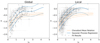 |
Fig. 1. Best-fit values of n as a function of τV for the fitted DES galaxies with DECam global (left panel) and local (right panel) griz photometry. Results for the different galaxies are shown in gray. A Gaussian Process Regression is shown in solid blue, with dashed blue lines defining a 68% credible interval. The mean relation found for similar simulated galaxies by Chevallard et al. (2013) is shown in dashed orange, with ±25% error margins shown in dotted orange. |
Despite some scatter, there is a clear correlation between the two quantities in both the global and the local cases, with larger optical depths corresponding to larger values of n, and thus shallower attenuation curves. The Spearman correlation coefficient between these two parameters for the DES data set is found to be 0.671 for the global measurements and 0.777 for the local measurements.
Comparing the global and the local fit results offers an interesting insight. As seen in Fig. 2, where we plot the deviations ΔτV = τVGlobal − τVLocal and Δn = nGlobal − nLocal as a function of the redshift z, the results for both fits appear fairly consistent, with median differences of ΔτV = 0.26 and Δn = 0.026.
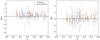 |
Fig. 2. Differences (Δ= Global-Local) between best-fit results for the parameters obtained with global and local DECam griz photometry for the DES galaxies, as a function of z. The left-hand side shows the results for τV and the right-hand side the ones for n. Results for the different galaxies are shown in gray. Binned means for each parameter are shown in orange, with error bars given by the standard deviation in each bin. |
There are some differences between the fits, as the values obtained for τV tend to be larger for the global photometry. There is also a large level of scatter present in the plots, with standard deviations of 0.712 for ΔτV and 0.575 for Δn. Furthermore, the percentage of galaxies for which the best-fit values are not compatible with each other is found to be 39.8% for τV and 36.0% for n.
The consistency of the observed correlation between the two result sets indicates that an aperture of 4 kpc is not sufficiently small to negate the geometrical effects associated with attenuation (see next section). Likely for the same reason, Kelsey et al. (2021) observe a similar consistency between global and local measurements, particularly when looking at U-R steps. In fact, the global and the local mass values obtained by Kelsey et al. (2021) indicate that, in some cases, a 4 kpc aperture is actually as large as the galaxy itself. This means one needs even smaller physical apertures to correctly estimate dust extinction at the SN location. However, this is difficult to achieve in practical terms due to instrument limitations. The fact that the results remain constant as the redshift increases indicates that the diminishing angular size of the aperture does not, in this case, play a large role in the results obtained.
We used either complete or partial additional global photometry in the NUV/FUV GALEX (Martin et al. 2005) and JHKs 2MASS (Skrutskie et al. 2006) filter bands for 33 of the studied galaxies. Although this additional set of measurements is not enough to draw any conclusions by itself, it is useful to confirm our previous fit results. Combining the new photometry with the griz global data points, a new set of fits was performed for these select galaxies. The differences between the new fit values for τV and n and the previously discussed griz results exhibit median relative values of ∼0.5% and ∼3%, with a standard deviation of 1.14 and 0.40, respectively. Despite the somewhat large value of scatter for τV, these values confirm the reliability of the results obtained with griz measurements.
4.2. Attenuation laws and galaxy orientation
For comparison, the mean relation obtained by Chevallard et al. (2013) for the overall correlation between τV and n for a set of simulated galaxies observed at different orientation angles is also shown in Fig. 1. This relation, which results from a slightly different attenuation law than the one discussed in this paper, differs somewhat from our data, with the simulated galaxies appearing in general redder. Even so, the overall qualitative tendency is the same as the one found for DES galaxies. Additionally, the recovered tendency also matches the behavior observed by both Leja et al. (2017) and Narayanan et al. (2018), which further suggests we are indeed recovering a physical relation. Given the agreement with the Chevallard et al. (2013) mean relation, it is reasonable to conclude that the overall correlation between the recovered dust parameters can be well explained by different galaxy orientations, as also described by Viaene et al. (2017) and Narayanan et al. (2018) and schematically illustrated on Fig. 3. This same trend between τV and n is also present for elliptical galaxies, as recently shown by Sachdeva & Nath (2022).
 |
Fig. 3. Schematic representation of dust attenuation for different galaxy orientations: Head-on (left panel) and Edge-on (right Panel). |
As stated by those works, cases with small τV, would mostly correspond to galaxies that are being observed face-on. In this case, we must consider both the photons emitted parallel and perpendicularly to the galactic plane. Photons emitted perpendicularly to the galactic plane (along the line of sight for a face-on galaxy) suffer minimal attenuation, independent of their wavelength. Additionally, we must also take into account photons emitted along the equatorial plane of a galaxy, which might be scattered away from the plane and into the line of sight. On one hand, blue photons tend to be scattered more forwardly, meaning they tend to remain confined to the galactic plane, eventually being fully absorbed (Chevallard et al. 2013). On the other hand, red photons tend to be scattered more isotropically and have a much lower interaction cross-section with dust, allowing them to more consistently escape the galactic plane (Chevallard et al. 2013). This means that an excess of red radiation is added to our line of sight, leading to higher values of reddening, reflected in more negative values for n.
The cases with a larger τV statistically correspond to an edge-on view of the galaxies. In these cases, radiation emitted from the deepest layers of the galaxy is greatly absorbed, independently of wavelength. The radiation reaching an observer is thus dominated by stars located in the outermost layers of the galaxy, unobscured stars and light scattered into the line of sight (Narayanan et al. 2018). This leads to an overall lower level of reddening and values of n closer to 0.
Galaxy orientation is not the only mechanism behind the correlation observed in Fig. 1, being mostly relevant for spiral galaxies. For elliptical galaxies, galaxy orientation is not an important factor. However, due to their general elliptical shape and overall low dust content, these particular galaxies end up exhibiting a behavior similar to the one observed for head-on spiral galaxies, leading to an overall large level of reddening. Additionally, different galaxies can have different intrinsic optical depths, which is one of the possible reasons for the scatter observed in the figure and the relations discussed in the next sections. It has also been recorded that there is some degree of degeneracy between galaxy geometry and intrinsic dust composition, which somewhat muddles the analysis (Viaene et al. 2017).
4.3. Attenuation laws and stellar mass
Another important factor in the characterization of the recovered attenuation laws is the possible correlations of the dust parameters with the stellar mass and age, which are plotted in Fig. 4. Despite some scatter, the relation between τV and log(M⋆/M⊙) seems to display two separate behaviors depending on the age of the corresponding stellar population. For younger galaxies, there is a steady increase of τV with log(M⋆/M⊙), which is in agreement with results obtained for star-forming galaxies by Salim et al. (2018), Garn & Best (2010), Zahid et al. (2013), as more massive galaxies have more gas and dust content with more active star formation. A separate tendency is observed for older galaxies, which tend to exhibit both larger masses and smaller optical depths. This matches what is expected for quiescent galaxies (Salim et al. 2018; Zahid et al. 2013), which have less dust and make up a large fraction of high-mass galaxies (Peng et al. 2010).
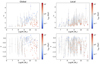 |
Fig. 4. Best-fit results for the dust parameters as a function of log(M⋆/M⊙) for the fitted DES galaxies with DECam global (left panels) and local (right panels) griz photometry. Plots for τV are shown in the top row, while results for n are shown in the bottom row. The best-fit for the age of each galaxy is plotted on a gradient from blue (younger) to red (older). |
The behavior of the two age populations is most prominent when looking at the global mass, but it is also apparent in the local case. This suggests a link not only with the total stellar mass of the galaxy, but also with the local stellar density, with older galaxies being generally more dense. It is also interesting to notice that a larger stellar density does not necessarily equate to a larger dust column density, as seen from the relatively low values of τV for high local masses. Although the large level of scatter complicates the analysis of the relation between n and log(M⋆/M⊙), we find that older galaxies tend to have more negative values of n and thus steeper attenuation curve slopes, which once again matches previous observations for quiescent galaxies (Salim et al. 2018; Wiseman et al. 2022).
Meldorf et al. (2023) examine the attenuation laws for a larger sample of DES SN Ia host galaxies and recover mostly the same trend for the relation between n and log(M⋆/M⊙). However, for the relation between AV and log(M⋆/M⊙), they only observe the roughly linear trend associated with star-forming galaxies and do not find a decrease of AV for massive galaxies. As previously stated, this decrease is expected due to the presence of high-mass quiescent galaxies (e.g., Zahid et al. 2013; Salim et al. 2018) and the trend we observe in Fig. 4 follows exactly those expectations.
For the global fit, we find a median RV = 2.762 (using Eq. (1)) with a standard deviation of 1.096, while for the local case we find a median RV = 2.612 with a standard deviation of 0.943. In addition, in Table 2 we list the values of RV obtained for both low- and high-mass galaxies, when adopting a standard step of log(Mstep/M⊙) = 10 for the global case and of log(Mstep/M⊙) = 9 for the local case. These step locations are based on the median masses for both sets of measurements. We find that, for the global case, low-mass galaxies have a considerably larger median RV, meaning that, for the same amount of dust, they appear to be systematically subject to a lower level of reddening. This once again points to the presence of massive quiescent galaxies in our sample, as for star-forming galaxies the value of RV is expected to increase with the stellar mass (Salim et al. 2018).
Median global and local RV values, standard deviations (STD) and standard errors (SE) for low- and high-mass galaxies.
Despite having standard deviations of RV ∼ 1, both of the populations exhibit low standard errors, with the difference between the median values of RV for each of them being significant at ∼2.5σ. Additionally, although the values do not match exactly, this order relation between low- and high-mass dust properties and the observed level of scatter is the same as the one recovered by Brout & Scolnic (2021) and González-Gaitán et al. (2021).
The results for the local case exhibit an opposite tendency, with a higher median RV for the high-mass population. This is probably due to the step location considered being too low, which does not allow the quiescent galaxies to meaningfully impact the high-mass population.
4.4. Host galaxy attenuation and SN Ia extinction
As discussed in Sect. 1, the phenomena governing dust extinction differ from those governing attenuation, as the geometrical effects related to the spatial distribution of dust and light sources cease to be relevant for the former, and only the amount and type of dust are important. It is thus crucial to take notice of the differences between the extinction laws affecting SNe Ia and the attenuation laws affecting their respective host galaxies.
With this in mind, in Fig. 5 we plot the best-fit values for RV and τV obtained for the attenuation laws for the DES host galaxies. As a term of comparison, we look at the extinction laws obtained by Mandel et al. (2011) for a set of SNe Ia at low redshift. We note that Burns et al. (2014) find a similar relation to Mandel, whereas recently Rose et al. (2022) find a flat distribution of RV for various extinction amounts of SNe Ia.
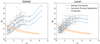 |
Fig. 5. Best-fit values of RV as a function of τV for the fitted DES galaxies with DECam Global (left panel) and Local (right panel) griz photometry. Results for the different galaxies are shown in gray. A Gaussian Process Regression is shown in solid blue, with dashed blue lines defining a 68% credible interval. The correlation found by Mandel et al. (2011) between these two quantities for the extinction laws of a set of nearby SNe Ia is shown in orange. |
It is clear that the extinction for SNe Ia and the attenuation for host galaxies exhibit two different tendencies. This is due to the fact that, for a point source, the effects arising from the dust-to-star geometry and observation angle are no longer relevant.
As shown in Sect. 4.1, the global and the local fit results are consistent, indicating that a 4 kpc aperture is not small enough to eliminate the dust-to-star geometry effects associated with dust attenuation.
For a more direct comparison with our sample, we can look at the light-curve parameters recovered for each of the DES SN Ia by Brout et al. (2019). In particular, looking at the Spearman correlation coefficients between the host galaxy attenuation parameters and the respective SN Ia light-curve parameters, shown in Table 3, it is clear that τV and n do not meaningfully correlate with the SN properties. In particular, there is no evident correlation with light-curve color, which once again points to the difficulty of using environmental attenuation properties to infer SN dust extinction. These results show that there is not a one-to-one relation between SN extinction and host galaxy attenuation, meaning it is difficult to take one as a proxy for the other.
Spearman correlation coefficients between the global and the local host galaxy attenuation parameters and the respective SN Ia light-curve parameters.
5. SN Ia cosmology
In this section, we focus on the effects of SN Ia standardization on the Hubble residuals. In particular, we examine whether there is evidence for a dust step in the data and how it compares to the more commonly used mass step.
5.1. SN Ia standardization
For each SN Ia, the SALT2 model (Guy et al. 2007, 2010) can be used to fit its light curve, returning values for the light-curve width x1, observed color at maximum c, and observed magnitude at maximum mB. Following the standardization formula introduced by Tripp (1998) with the addition of a δμbias term, the corrected distance modulus μ for each SN is then given by:

where α, β and M are nuisance parameters obtained from a cosmological fit, describing the shape–luminosity and color–luminosity corrections, as well as the absolute magnitude of a fiducial SN Ia with x1 = 0 and c = 0, respectively, and δμbias is a 1D bias correction term, introduced as a function of the redshift and obtained from survey simulations. To account for the mass step, an additional correction term δμM, dependent on the host galaxy mass M⋆, is usually added to the previous expression (e.g., Betoule et al. 2014).
For the cosmological fit, we take advantage of the fact that μ can be expressed as a function of the luminosity distance dL which, for a Friedmann-Robertson-Walker cosmology, only depends on the cosmological parameters and the redshift (Riess et al. 1998). Generally, the model parameters H0 and Ωm are kept as free parameters, along with α, β and M. By minimizing the Hubble residuals Δμ = μ − μmodel these parameters could therefore be constrained via the fit. In this work, the cosmological parameters are kept fixed to Ωm = 0.3, ΩΛ = 0.7, w = −1 and H0 = 70 km s−1 Mpc−1, as we are mainly interested in the effects of dust and the color–luminosity correction on the standardizations.
For the standardization fits we use the EMCEE package to apply a Bayesian fitting procedure, with overall flat priors for the fit parameters. The likelihood function is defined as:
where σ2 is defined as:
In the previous expression, σmB, σx1 and σc are the uncertainties associated with each of the light-curve fit parameters, σmB, c, σmB, x1 and σx1, c are their covariance terms and σint is a parameter that accounts for possible intrinsic variations in a SN Ia’s luminosity. We fix σint = 0.107, following the value obtained by González-Gaitán et al. (2021)12.
It is known that the likelihood defined by Eq. (3) can introduce biases into the recovered fit parameters (Kessler & Scolnic 2017). However, as our main objective is a wholesale comparison between two standardization processes using the same likelihood, these biases should not be of much relevance. This comparison is focused on the improvement of the RMS of the Hubble residuals with respect to the fiducial model.
The cosmological fit parameters recovered following this method for the Tripp standardization are listed in Table 4, with the corresponding values of RMS for the residuals also shown. The light-curve parameters recovered for each of the DES SN Ia by Brout et al. (2019) using the SALT2 model, as well as the corresponding 1D bias corrections, were used for the fits.
A separate “Fixed-Extinction” standardization, in which the extinction contribution to the color–luminosity correction can be fixed using our prior measurements of RV and E(B − V) for the host galaxies from Sect. 4, is described in Appendix C. For this standardization, an additional free intrinsic color–luminosity parameter βint is introduced. The corresponding fit parameters for this standardization are also displayed in Table C.1. It however results in much worse fits, as can be seen in the large RMS.
5.2. Hubble residuals steps
We now examine possible “steps” in the Hubble residuals for the Tripp standardization, associated with both the local and global properties of the host. We investigate “steps” associated with both the host mass and dust properties.
To look for a step, we divide the Hubble residuals into two populations, according to the properties of the SN host. By varying the threshold values at which the population division is made, we can determine the optimal location for the step. This can be done by optimizing several quantities, namely the step magnitude, the step significance and the ΔRMS with respect to the fiducial Tripp standardization.
For a description with two populations A and B, the step magnitude γ is defined as the difference between the mean values of the Hubble residuals for each of the two populations, while the step significance is defined as the ratio between the step magnitude and the step error σstep, given by:
where NA and NB are the number of data points in each of the populations and σA and σB are the STDs for each of the populations.
ΔRMS is defined as the difference between the standard RMSsingle obtained when considering the Hubble residuals as a single population and the RMSdual obtained when considering them as two separate populations, each with a separate mean and divided at the step in mass or dust. Thus, the larger the value of ΔRMS, the more the two-population description is favored.
5.2.1. The mass step
When considering a mass step, the two populations are taken to be SNe Ia originating in either low- or high-mass galaxies. Following the procedure detailed in the previous section, we look for a division in mass between two populations that maximizes the step magnitude, its significance and ΔRMS. The optimal step values obtained are shown in Table 5, with the corresponding values of RMSdual also shown. The optimal values are also plotted in Fig. 6. In addition, in Fig. 7 the Hubble residuals for the SNe are plotted, as well as the corresponding optimal steps and the mean values for log(M⋆/M⊙) and Δμ found for each mass bin.
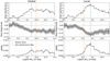 |
Fig. 6. Variation of the mass step with step location for the Tripp standardization, for the global (left panels) and the local (right panels) cases. The top panel shows the significance of the step in σ, the middle panel shows the magnitude of the step in solid black, with the gray region showing the uncertainty, and the lower panel shows ΔRMS. In these three panels, the location of the step of maximum significance is shown in blue and the median mass of the sample is shown in orange. Inspired by Kelsey et al. (2021). |
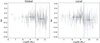 |
Fig. 7. Hubble residuals Δμ for the DES SNe Ia as a function of the stellar mass for the respective host galaxies, plotted in gray. The optimal step locations, as recorded in Table 5 are shown in dashed blue. The blue dots show the mean values of log(M⋆/M⊙) and Δμ in each bin, with the error in the x-axis given by the standard deviation. |
Mass-step significance (in σ), magnitude (γM), ΔRMS and RMSdual for the Tripp and Tripp+δμD standardizations.
We obtain optimal steps that are not only both significant at > 3σ, but also correspond to the best improvement in RMS. Additionally, both step locations and their respective significance levels roughly match the results obtained by Kelsey et al. (2021) for this data set, pointing to the existence of a mass step for the Tripp standardization.
In Table 2 we present the RV values for both low- and high-mass galaxy populations, as defined by the step values recovered for the Tripp standardization. We once again find that, for the global case, low-mass galaxies have a larger median RV, with the difference between the two populations being significant at ∼2σ. We also find that, as the local step location shifts to a higher mass, the same tendency starts to be observed in this case. In the next section, we further explore the discrepancy between these populations, analyzing whether it can be described by a dust step.
5.2.2. The dust step
Having established the presence of a mass step, we next look at whether evidence for a step related to the dust content of a SN host can be found in the data for the Tripp standardization. There are some differences to the approach discussed for the mass step. First, while the stellar mass of a galaxy can be described by a single parameter, M⋆, dust attenuation is parameterized by two parameters, τV and n. To account for this fact and ensure we are accurately accounting for a possible dust step, we adopt a two-dimensional population division. One-dimensional steps in both τV and n were attempted, but they were found not to be very significant (∼2σ). Second, we consider three different population splits to fully cover the τV − n parameter space. These are chosen to preserve a two-population division, thus making the mass and dust steps more comparable.
The three splits, schematically represented in Fig. 8, are: one population consisting of SNe Ia originating in low attenuation, high reddening galaxies (Region 1 in Fig. 8) and another consisting of the remaining SNe, defined as the First Split; one population consisting of SNe Ia originating in low attenuation, low reddening galaxies (Region 2 in Fig. 8) and another consisting of the remaining SNe, defined as the Second Split; one population consisting of SNe Ia originating in high attenuation, low reddening galaxies (Region 3 in Fig. 8) and another consisting of the remaining SNe, defined as the Third Split. There is also a fourth possible split that is not considered, as the region with high attenuation and high reddening galaxies (Region 4 in Fig. 8) is very sparsely populated.
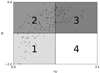 |
Fig. 8. Schematic representations of the regions singled out by each of the proposed dust-step splits in the τV − n parameter space. The best-fit values of n as a function of τV for the fitted DES galaxies with global griz photometry are shown for reference. The dashed lines only represent possible division points for the populations, with the actual optimal values recorded in in Table 6. |
The optimal step values for the First, Second and Third Splits are shown in Table 6. The Second Split results in the best significance and ΔRMS values, which means it is by far the most favorable for a dust step. We can further analyze this particular case by taking a closer look at the variation of the step magnitude, significance and ΔRMS, plotted in Fig. 9. We can see that, not only are the optimal step locations very narrow, but they also exhibit clear delimitations for both dust parameters, suggesting we are indeed encountering a two-dimensional step. This is particularly apparent when using global data. In the local case, there appear to be two possible step locations. We take the optimal step to be the one that maximizes ΔRMS. The significance, magnitude and ΔRMS values obtained for the optimal global dust step are very close to those recovered for the optimal global mass step, even though the dust step ends up being slightly stronger. In particular, the dust steps are significant at > 4σ, which matches the results obtained by Meldorf et al. (2023) for DES-SN host galaxies.
 |
Fig. 9. Variation of the Second Split dust step with the step location (position in τV − n grid) for the Tripp standardization. Results from global measurements are shown on the left, while those from local measurements are shown on the right. The top panel shows the significance of the step in σ, the middle panel shows the magnitude of the step and the lower panel shows ΔRMS. This last quantity is defined as the difference between the RMSsingle obtained for a single population mean description and the RMSdual obtained for a dual population mean description with a step. |
Dust-step significance (in σ), magnitude (γD), ΔRMS and RMSdual for the Tripp and Tripp+δμM standardizations.
5.2.3. Mass and dust step comparison
For a more rigorous SN standardization, the steps recovered in the previous sections can be introduced into the usual Tripp standardization. In particular, we do this to ascertain whether correcting for one of the steps eliminates the other one. In such cases, the mass step takes the form:
where Mstep is the optimal step location and γM the corresponding step magnitude recovered in Sect. 5.2.1 and recorded in Table 5. For the Second Split, the dust step takes the form:
where τVstep and nstep are the optimal step locations and γD the corresponding step magnitude recovered in Sect. 5.2.2 and recorded in Table 6.
It is clear from Fig. 10 that the two mass and dust populations do not exactly align. In fact, higher-mass galaxies tend to concentrate on the inside of the τV − n curve, while less massive galaxies concentrate on the outside. This is particularly apparent in the local case. This discrepancy points to the fact that the recovered dust step is not merely analogous to the mass step, as might initially be presumed, given its magnitude, significance and ΔRMS.
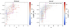 |
Fig. 10. Best-fit values of n as a function of τV for the fitted DES galaxies with DECam global (left panel) and local (right panel) griz photometry. The corresponding value of log(M⋆/M⊙) is plotted on a gradient from blue (lower mass) to red (higher mass). The optimal step for the Second Split is also shown in purple. |
For a more detailed look at this discrepancy, we can add a dust step in the form of Eq. (7) to the Hubble residuals for the Tripp standardization. To do so, we fix the values of γD, τVstep and nstep to those previously obtained in Sect. 5.2.2 for the optimal dust step, as recorded in Table 6. Following a similar procedure as the one applied in Sect. 5.2.1, we once again recover the optimal mass step, shown in Table 5. It should be noted that, when looking for this new mass step, the baseline for comparison is not the case with no step, but rather the case already corrected for the dust step.
For the local case, the optimal mass-step location remains unchanged. For the global case, however, there is a big change in the maximum significance step location, which happens because the previous optimal step significance drops slightly below the level of the new maximum. For the sake of consistency, we keep the same step location. Even so, the new maximum significance step, log(M⋆/M⊙) = 10.51, has a significance of 3.20.
It is clear that the introduction of the dust-step correction lowers both the significance, magnitude and ΔRMS of the recovered mass steps. This drop in ΔRMS should not be taken to mean that the inclusion of both steps results in an overall worse RMS when compared with a single step case. Rather, it signifies that the addition of a mass step to a set of Hubble residuals already corrected with a dust step results in a lower improvement in RMS than the one seen for the same mass step applied to Hubble residuals with no prior step correction. In this sense, the initial dust-step correction appears to also be partially correcting for the mass effect. However, it cannot be said that the mass step has been removed in either case. Thus, while offering some improvement, the addition of this dust-step term to the standardization is not capable of fully eliminating the mass step by itself.
In the same way, we can look at the recovered dust step in the case of a Tripp+mass-step standardization, in which the mass step recovered in Sect. 5.2.1 is used. The values relating to these steps are shown in Table 6. Once again, it is clear that the structure of the original steps is preserved, while the significance, magnitude and ΔRMS are again found to be lower. Thus, the addition of a mass-step term in the standardization is also not capable of fully eliminating the dust step by itself.
Thus, it seems reasonable to conclude that the mass and dust steps are two overlapping phenomena that nevertheless do not fully coincide. This points to the fact that the origin of the mass step may not be entirely driven by host dust properties. A further exploration of the relation between the two steps is offered in Appendix D, where both μM and μD are treated as free parameters in the cosmological fit. This confirms that the two steps are not analogous, as both are significantly different from zero for the best-fit cosmological model.
Looking at a bigger sample of DES host galaxies that includes SN Ia photometry, Meldorf et al. (2023) find that the inclusion of a dust-step correction is sufficient to correct the mass step. The discrepancy between this and our results is most likely due to the different mass to dust relations recovered from the host galaxy fits, as discussed in Sect. 4.3.
5.2.4. SN color and Hubble residuals steps
Although we do not find any direct relation between SN color and the galaxy dust parameters (Sect. 4.4), we explore the relation between SN color and the Hubble residuals, similarly to what is done in (e.g., Brout & Scolnic 2021). The SNe were divided into two populations: Blue SNe (c < 0) and Red SNe (c > 0). For an easier comparison with the previous results, the optimal locations found in Sects. 5.2.1 and 5.2.2 were preserved. These results are shown in Tables 7 and 8, for the mass and dust steps, respectively.
Mass-step significance (in σ), magnitude (γM), ΔRMS and RMSdual for different color populations.
Dust-step significance (in σ), magnitude (γD), ΔRMS and RMSdual for different color populations.
It is clear from the significance, magnitude and ΔRMS values that both steps are much more pronounced for the red SNe, which matches the results obtained by Kelsey et al. (2021) and Brout & Scolnic (2021). This difference between the two populations points once again to a relation between dust reddening and the Hubble residuals steps, assuming most of the color variation for SNe stems from dust. However, it has also been suggested that there is possible indirect evidence of environmental variation of intrinsic SN color, particularly related to ejecta velocity (e.g., Pan 2020; Wang et al. 2013; Cartier et al. 2011), which could also be playing a partial role in this case.
Finally, similarly to what was done in Sect. 5.2.3, we examine what happens to the mass step if the dust step is corrected for and vice versa. Depending on the population in question, we use either the steps recovered for the blue or the red SNe. The results remain consistent with what we have shown before, with neither of the steps being able to fully account for the other, regardless of the color of the SNe considered.
6. Discussion
Several key results obtained in this work appear to support the link between environmental dust properties and the mass step.
First, the mass–τV and mass–n relations, shown in Fig. 4, make it clear that different galaxy mass populations are subject to different dust contents and dust laws. This fact is most clearly expressed in the results displayed in Table 2, where it is shown that the RV values for low- and high-mass galaxies exhibit significant differences, which agrees with previous results (e.g., Salim et al. 2018; Brout & Scolnic 2021; González-Gaitán et al. 2021).
Second, in Sect. 5.2.3 we show that adding a dust step to a set of mass-step corrected Hubble residuals results in lower significances, magnitudes and ΔRMS than the ones obtained for the same step when no initial correction is present, and vice versa. This shows that the effects in mass and dust are at least partially related and that correcting for one also partly corrects for the other.
Third, as shown in Sect. 5.2.4, both the mass and dust steps are found to have much higher values of significance, magnitude and ΔRMS for red SNe (c > 0), when compared to blue SNe (c < 0). Presuming that red SNe are also the most extinguished, we have yet another link between dust and the mass step.
However, the color variations among SNe are not only a product of dust extinction, but can also originate from intrinsic differences between the SNe (e.g., Conley et al. 2007). For this reason, the fact that the mass step is found to be more prominent for red SNe might also indicate a relation between this effect and the SN intrinsic color (Pan 2020; Wang et al. 2013).
Another result that points against dust as the sole driver for the mass step is the overall lack of correlation found between SN color and the corresponding host galaxy attenuation parameters, as recorded in Table 3. This again suggests that the differences in the mass step between different color SNe might actually be due to intrinsic factors. Another possibility is that global and local (4 kpc) environmental dust properties might be very poor proxies of the real dust extinction at the SN site.
This last point is further strengthened by the fact that, as shown in Fig. 5, extinction and attenuation display very different behaviors, pointing to different physical effects. This also explains why the proposed “Fixed-Extinction” Standardization, discussed in Appendix C, gives such poor results.
Furthermore, while it is true that there appears to be an overlap between the two steps, we show that accounting for one of them does not fully remove the other, suggesting that there might be other factors at play, not directly related to dust.
In general, our results seem to point to the fact that the mass step might not have a fully dust-related origin, despite the evidence for at least a partial link between the two. As stated before, it is possible that a partial cause of the observed effect lies instead in intrinsic differences between SNe Ia that come about due to different progenitors. The fact that the stellar age seems to be quite important in the relations between the attenuation law and the mass (see Fig. 4) shows that the situation is more complex and agrees with other works that show the importance of age in the mass step (e.g., Rigault et al. 2020; Rose et al. 2022; Wiseman et al. 2022). In this sense, both the environmental mass and dust might be acting as imperfect proxies for the different types of progenitors, explaining the behavior we observe.
Finally, while dust might indeed be the origin of the mass step, a two-dimensional environmental dust step might be an overly simplistic way to look at the relation between these two quantities. One might need either direct extinction data for each supernova or a better way to isolate the different mass/dust populations.
7. Conclusions
In this work, we have explored ways to better probe the dust contents of SN Ia host galaxies as well as how to better make use of this information for SN standardization. Our major findings are:
-
We have shown through simulations that DECam griz photometry is mostly sufficient to recover dust parameters for simulated SN Ia host galaxies, while discrepancies and degeneracies among other parameters do not significantly affect inferred dust properties. We found that in using both global and local DECam griz photometry, we can recover dust properties for host galaxies that are consistent with literature predictions from both simulations and observations. We find a relation for the dust attenuation slope with the dust optical depth, both locally and globally, that is best explained with varying star-to-dust geometry with a galaxy orientation. Most importantly, we show that dust properties vary greatly across different galaxies, meaning a universal value of RV = 3.1 or a universal SN Ia β correction are assumptions that are too simplistic.
-
The relation between the attenuation parameters is found to be very different from the extinction relations obtained directly for SNe Ia, making the comparison between the two somewhat difficult. This difference is mainly due to the effects related to star-to-dust geometry that become relevant when dealing with extended objects, such as SN host galaxies.
-
We find two different relations between a galaxy’s stellar mass and its dust properties, depending on the age of the corresponding stellar population. For younger galaxies, there is a steady increase of τV and n with log(M⋆/M⊙), while older galaxies tend to exhibit both larger masses and smaller optical depths. A similar behavior for the two age populations can be seen when considering the local mass, pointing to an analogous relation between the results observed for the global stellar mass and the local stellar density. This population mix results in the observation that low-mass galaxies tend to have larger values of RV, meaning that, for the same amount of dust, these galaxies are systematically subject to a lower level of reddening. For both mass populations, the scatter in RV is ∼1. All of these results match previous literature observations.
-
We conclude that an alternative SN Ia standardization, incorporating both the RV and E(B − V) values obtained for the respective host galaxies to approximate and fix SN extinction, results in a worse cosmological fit. This is very likely a consequence of the differences between host galaxy attenuation and SN Ia extinction, meaning the values for βRV and E(B − V) for the SNe Ia cannot be correctly determined. The lack of correlation between the host attenuation parameters and the respective SN light-curve parameters also points to this fact. This remains true when carrying out local studies (4 kpc), showing that even smaller apertures are needed to avoid the geometrical effects of dust attenuation.
-
We show there is evidence for a two-dimensional dust step, which, for the global case, results in roughly the same significance, magnitude, and residual RMS recovered for the mass step, hinting at a relation between the two. In particular, this dust step is significant at > 4σ. Furthermore, we show that these two steps are not completely analogous and that accounting for one of them in the SN standardization does not necessarily fully eliminate the other.
-
We find that both the mass and dust steps are much more pronounced for red SNe Ia (c > 0), which once again suggests a link between dust reddening and the Hubble residual steps.
Thus, we conclude that the need for the mass-step correction cannot be completely eliminated using only host galaxy dust data. This is true for both an alternative SN standardization, in which the color–luminosity relation is constrained with host attenuation, and for a SN standardization with a dust-step correction.
Cornerplots and SED fit plots for the host galaxies can be found at https://github.com/SN-CRISP/DES-SN_Host-Galaxies
A cosmological fit with a free σint is explored in Appendix D.
Acknowledgments
J.D., S.G.G., A.M. and A.P.A. acknowledge support by FCT under Project CRISP PTDC/FIS-AST-31546/2017 and Project No. UIDB/00099/2020. L.G. acknowledges financial support from the Spanish Ministerio de Ciencia e Innovación (MCIN), the Agencia Estatal de Investigación (AEI) 10.13039/501100011033, and the European Social Fund (ESF) “Investing in your future” under the 2019 Ramón y Cajal program RYC2019-027683-I and the PID2020-115253GA-I00 HOSTFLOWS project, from Centro Superior de Investigaciones Científicas (CSIC) under the PIE project 20215AT016, and the program Unidad de Excelencia María de Maeztu CEX2020-001058-M. L.K. thanks the UKRI Future Leaders Fellowship for support through the grant MR/T01881X/1. Computations were performed at the cluster “Baltasar-Sete-Sóis” and supported by the H2020 ERC Consolidator Grant “Matter and strong field gravity: New frontiers in Einstein’s theory” grant agreement no. MaGRaTh-646597. P.W. acknowledges support from the Science and Technology Facilities Council (STFC) grant ST/R000506/1. Funding for the DES Projects has been provided by the U.S. Department of Energy, the U.S. National Science Foundation, the Ministry of Science and Education of Spain, the Science and Technology Facilities Council of the United Kingdom, the Higher Education Funding Council for England, the National Center for Supercomputing Applications at the University of Illinois at Urbana-Champaign, the Kavli Institute of Cosmological Physics at the University of Chicago, the Center for Cosmology and Astro-Particle Physics at the Ohio State University, the Mitchell Institute for Fundamental Physics and Astronomy at Texas A&M University, Financiadora de Estudos e Projetos, Fundação Carlos Chagas Filho de Amparo á Pesquisa do Estado do Rio de Janeiro, Conselho Nacional de Desenvolvimento Científico e Tecnológico and the Ministério da Ciência, Tecnologia e Inovação, the Deutsche Forschungsgemeinschaft and the Collaborating Institutions in the Dark Energy Survey. The Collaborating Institutions are Argonne National Laboratory, the University of California at Santa Cruz, the University of Cambridge, Centro de Investigaciones Energéticas, Medioambientales y Tecnológicas-Madrid, the University of Chicago, University College London, the DES-Brazil Consortium, the University of Edinburgh, the Eidgenössische Technische Hochschule (ETH) Zürich, Fermi National Accelerator Laboratory, the University of Illinois at UrbanaChampaign, the Institut de Ciéncies de l’Espai (IEEC/CSIC), the Institut de Física d’Altes Energies, Lawrence Berkeley National Laboratory, the Ludwig-Maximilians Universität München and the associated Excellence Cluster Universe, the University of Michigan, the National Optical Astronomy Observatory, the University of Nottingham, The Ohio State University, the University of Pennsylvania, the University of Portsmouth, SLAC National Accelerator Laboratory, Stanford University, the University of Sussex, Texas A&M University, and the OzDES Membership Consortium. Based in part on observations at Cerro Tololo Inter-American Observatory, National Optical Astronomy Observatory, which is operated by the Association of Universities for Research in Astronomy (AURA) under a cooperative agreement with the National Science Foundation. The DES data management system is supported by the National Science Foundation under Grant Numbers AST-1138766 and AST-1536171. The DES participants from Spanish institutions are partially supported by MINECO under grants AYA2015-71825, ESP2015-66861, FPA2015-68048, SEV-2016-0588, SEV2016-0597, and MDM-2015-0509, some of which include ERDF funds from the European Union. IFAE is partially funded by the CERCA program of the Generalitat de Catalunya. Research leading to these results has received funding from the European Research Council under the European Union’s Seventh Framework Program (FP7/2007-2013) including ERC grant agreements 240672, 291329, and 306478. We acknowledge support from the Brazilian Instituto Nacional de Ciência e Tecnologia (INCT) e-Universe (CNPq grant 465376/2014-2). This manuscript has been authored by Fermi Research Alliance, LLC under Contract No. DE-AC02-07CH11359 with the U.S. Department of Energy, Office of Science, Office of High Energy Physics.
References
- Abbott, T., Abdalla, F. B., Aleksić, J., et al. 2016, MNRAS, 460, 1270 [Google Scholar]
- Abbott, T. M. C., Abdalla, F. B., Allam, S., et al. 2018, ApJS, 239, 18 [Google Scholar]
- Abbott, T. M. C., Allam, S., Andersen, P., et al. 2019, ApJ, 872, L30 [Google Scholar]
- Bertin, E., & Arnouts, S. 1996, A&AS, 117, 393 [NASA ADS] [CrossRef] [EDP Sciences] [Google Scholar]
- Betoule, M., Kessler, R., Guy, J., et al. 2014, A&A, 568, A22 [NASA ADS] [CrossRef] [EDP Sciences] [Google Scholar]
- Bradley, L., Sipocz, B., Robitaille, T., et al. 2019, https://zenodo.org/records/2533376 [Google Scholar]
- Brout, D., & Scolnic, D. 2021, ApJ, 909, 26 [NASA ADS] [CrossRef] [Google Scholar]
- Brout, D., Scolnic, D., Kessler, R., et al. 2019, ApJ, 874, 150 [NASA ADS] [CrossRef] [Google Scholar]
- Burns, C. R., Stritzinger, M., Phillips, M. M., et al. 2014, ApJ, 789, 32 [Google Scholar]
- Calzetti, D. 2001, PASP, 113, 1449 [Google Scholar]
- Calzetti, D., Kinney, A. L., & Storchi-Bergmann, T. 1994, ApJ, 429, 582 [Google Scholar]
- Calzetti, D., Armus, L., Bohlin, R. C., et al. 2000, ApJ, 533, 682 [NASA ADS] [CrossRef] [Google Scholar]
- Cardelli, J. A., Clayton, G. C., & Mathis, J. S. 1989, ApJ, 345, 245 [Google Scholar]
- Cartier, R., Förster, F., Coppi, P., et al. 2011, A&A, 534, L15 [NASA ADS] [CrossRef] [EDP Sciences] [Google Scholar]
- Chevallard, J., Charlot, S., Wandelt, B., & Wild, V. 2013, MNRAS, 432, 2061 [CrossRef] [Google Scholar]
- Condon, J. J., & Matthews, A. M. 2018, PASP, 130, 073001 [NASA ADS] [CrossRef] [Google Scholar]
- Conley, A., Carlberg, R. G., Guy, J., et al. 2007, ApJ, 664, L13 [NASA ADS] [CrossRef] [Google Scholar]
- Conroy, C., & Gunn, J. E. 2010, ApJS, 712, 833 [NASA ADS] [Google Scholar]
- Conroy, C., Gunn, J. E., & White, M. 2009, ApJS, 699, 486 [NASA ADS] [Google Scholar]
- Dhawan, S., Jha, S. W., & Leibundgut, B. 2018, A&A, 609, A72 [NASA ADS] [CrossRef] [EDP Sciences] [Google Scholar]
- Draine, B. T. 2003, ARA&A, 41, 241 [NASA ADS] [CrossRef] [Google Scholar]
- Erickson, C. 2021, GauPro: Gaussian Process Fitting, R package version 0.2.4 [Google Scholar]
- Feeney, S. M., Mortlock, D. J., & Dalmasso, N. 2018, MNRAS, 476, 3861 [NASA ADS] [CrossRef] [Google Scholar]
- Fitzpatrick, E. L. 1999, PASP, 111, 63 [Google Scholar]
- Flaugher, B., Diehl, H. T., Honscheid, K., et al. 2015, AJ, 150, 150 [Google Scholar]
- Foreman-Mackey, D., Hogg, D. W., Lang, D., & Goodman, J. 2013, PASP, 125, 306 [Google Scholar]
- Foreman-Mackey, D., Sick, J., & Johnson, B. 2014, https://doi.org/10.5281/zenodo.12157 [Google Scholar]
- Garn, T., & Best, P. N. 2010, MNRAS, 409, 421 [Google Scholar]
- González-Gaitán, S., de Jaeger, T., Galbany, L., et al. 2021, MNRAS, 496, 3402 [Google Scholar]
- Guy, J., Astier, P., Baumont, S., et al. 2007, A&A, 466, 11 [NASA ADS] [CrossRef] [EDP Sciences] [Google Scholar]
- Guy, J., Sullivan, M., Conley, A., et al. 2010, A&A, 523, A7 [NASA ADS] [CrossRef] [EDP Sciences] [Google Scholar]
- Johansson, J., Cenko, S. B., Fox, O. D., et al. 2021, ApJ, 923, 237 [NASA ADS] [CrossRef] [Google Scholar]
- Johnson, B. D., Leja, J., Conroy, C., & Speagle, J. S. 2021, ApJS, 254, 22 [NASA ADS] [CrossRef] [Google Scholar]
- Jones, D. O., Mandel, K. S., Kirshner, R. P., et al. 2022, ApJ, 933, 172 [NASA ADS] [CrossRef] [Google Scholar]
- Kelly, P. L., Hicken, M., Burke, D. L., Mandel, K. S., & Kirshner, R. P. 2010, ApJ, 715, 743 [Google Scholar]
- Kelsey, L., Sullivan, M., Smith, M., et al. 2021, MNRAS, 501, 4861 [NASA ADS] [CrossRef] [Google Scholar]
- Kessler, R., & Scolnic, D. 2017, ApJ, 836, 56 [Google Scholar]
- Kriek, M., & Conroy, C. 2013, ApJ, 775, L16 [NASA ADS] [CrossRef] [Google Scholar]
- Kroupa, P. 2001, MNRAS, 322, 231 [NASA ADS] [CrossRef] [Google Scholar]
- Lampeitl, H., Smith, M., Nichol, R. C., et al. 2010, ApJ, 722, 566 [Google Scholar]
- Leja, J., Johnson, B. D., Conroy, C., Dokkum, P. G. V., & Byler, N. 2017, ApJ, 837, 170 [NASA ADS] [CrossRef] [Google Scholar]
- Lequeux, J., Maurice, E., Prevot-Burnichon, M. L., Prevot, L., & Rocca-Volmerange, B. 1982, A&A, 113, L15 [NASA ADS] [Google Scholar]
- Mandel, K. S., Narayan, G., & Kirshner, R. P. 2011, ApJ, 731, 120 [CrossRef] [Google Scholar]
- Martin, D. C., Fanson, J., Schiminovich, D., et al. 2005, ApJ, 619, L1 [Google Scholar]
- Meldorf, C., Palmese, A., Brout, D., et al. 2023, MNRAS, 518, 1985 [Google Scholar]
- Nandy, K., Morgan, D. H., Willis, A. J., Wilson, R., & Gondhalekar, P. M. 1981, MNRAS, 196, 955 [CrossRef] [Google Scholar]
- Narayanan, D., Conroy, C., Davé, R., Johnson, B. D., & Popping, G. 2018, ApJ, 869, 70 [Google Scholar]
- Nataf, D. M., Gonzalez, O. A., Casagrande, L., et al. 2015, MNRAS, 456, 2692 [Google Scholar]
- Noll, S., Burgarella, D., Giovannoli, E., et al. 2009, A&A, 507, 1793 [NASA ADS] [CrossRef] [EDP Sciences] [Google Scholar]
- Pan, Y.-C. 2020, ApJ, 895, L5 [NASA ADS] [CrossRef] [Google Scholar]
- Peng, Y.-J., Lilly, S. J., Kovač, K., et al. 2010, ApJ, 721, 193 [Google Scholar]
- Perlmutter, S., Aldering, G., Goldhaber, G., et al. 1999, ApJS, 517, 565 [NASA ADS] [Google Scholar]
- Phillips, M. M. 1993, ApJ, 413, L105 [Google Scholar]
- Ponder, K. A., Wood-Vasey, W. M., Weyant, A., et al. 2021, ApJ, 923, 197 [NASA ADS] [CrossRef] [Google Scholar]
- Popovic, B., Brout, D., Kessler, R., & Scolnic, D. 2021, ArXiv e-prints [arXiv:2112.04456] [Google Scholar]
- Riess, A. G., Filippenko, A. V., Challis, P., et al. 1998, AJ, 116, 1009 [Google Scholar]
- Riess, A. G., Casertano, S., Yuan, W., Macri, L. M., & Scolnic, D. 2019, ApJ, 876, 85 [Google Scholar]
- Riess, A. G., Yuan, W., Casertano, S., Macri, L. M., & Scolnic, D. 2020, ApJ, 896, L43 [Google Scholar]
- Rigault, M., Brinnel, V., Aldering, G., et al. 2020, A&A, 644, A176 [NASA ADS] [CrossRef] [EDP Sciences] [Google Scholar]
- Rose, B. M., Popovic, B., Scolnic, D., & Brout, D. 2022, MNRAS, 516, 4822 [NASA ADS] [CrossRef] [Google Scholar]
- Sachdeva, S., & Nath, B. B. 2022, MNRAS, 513, L63 [NASA ADS] [CrossRef] [Google Scholar]
- Salim, S., & Narayanan, D. 2020, ARA&A, 58, 529 [NASA ADS] [CrossRef] [Google Scholar]
- Salim, S., Boquien, M., & Lee, J. C. 2018, ApJ, 859, 11 [Google Scholar]
- Schlafly, E. F., Meisner, A. M., Stutz, A. M., et al. 2016, ApJ, 821, 78 [NASA ADS] [CrossRef] [Google Scholar]
- Schlegel, D. J., Finkbeiner, D. P., & Davis, M. 1998, ApJ, 500, 525 [Google Scholar]
- Scolnic, D. M., Jones, D. O., Rest, A., et al. 2018, ApJ, 859, 101 [NASA ADS] [CrossRef] [Google Scholar]
- Skrutskie, M. F., Cutri, R. M., Stiening, R., et al. 2006, AJ, 131, 1163 [NASA ADS] [CrossRef] [Google Scholar]
- Smith, M., Sullivan, M., Wiseman, P., et al. 2020, MNRAS, 494, 4426 [Google Scholar]
- Sullivan, M., Conley, A., Howell, D. A., et al. 2010, MNRAS, 406, 782 [NASA ADS] [Google Scholar]
- Thorp, S., Mandel, K. S., Jones, D. O., Ward, S. M., & Narayan, G. 2021, MNRAS, 524, 235 [Google Scholar]
- Tripp, R. 1998, A&A, 331, 815 [NASA ADS] [Google Scholar]
- Uddin, S. A., Burns, C. R., Phillips, M. M., et al. 2020, ApJ, 901, 143 [NASA ADS] [CrossRef] [Google Scholar]
- Viaene, S., Sarzi, M., Baes, M., Fritz, J., & Puerari, I. 2017, MNRAS, 472, 1286 [NASA ADS] [CrossRef] [Google Scholar]
- Wang, X., Wang, L., Filippenko, A. V., Zhang, T., & Zhao, X. 2013, Science, 340, 170 [NASA ADS] [CrossRef] [Google Scholar]
- Wiseman, P., Smith, M., Childress, M., et al. 2020, MNRAS, 495, 4040 [Google Scholar]
- Wiseman, P., Vincenzi, M., Sullivan, M., et al. 2022, MNRAS, 515, 4587 [NASA ADS] [CrossRef] [Google Scholar]
- Zahid, H. J., Yates, R. M., Kewley, L. J., & Kudritzki, R. P. 2013, ApJ, 763, 92 [NASA ADS] [CrossRef] [Google Scholar]
Appendix A: Host galaxy mass comparison
In this appendix, we compare the stellar mass values recovered by Kelsey et al. (2021) for the DES-SN host galaxies with the values obtained using our methodology, with five-parameter sampling and no initial minimization. The results are displayed in Fig. A.1.
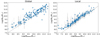 |
Fig. A.1. Comparison between the stellar mass values obtained by Kelsey et al. (2021) for the host galaxies of the DES-SN sample and the masses recovered using a five-parameter sampling with no initial minimization. In both cases, fits were performed using global (Left panel) and local (Right panel) DECam griz photometry. The results are shown in blue. A dashed line with y = x is also shown. |
As previously stated, the recovered values exhibit a median relative difference of ∼4% in relation to the values computed by Kelsey et al. (2021), in both the global and the local cases. There is, however, a clear bias between the two fitting methods, as the fitting methodology discussed in this paper returns systematically higher-mass values. Even so, as discussed in 3, where we purposely change the mass values by 4%, this discrepancy does not have a noticeable impact on the recovered dust parameters.
Appendix B: Host galaxy simulations
In this appendix, we present a more complete view of the various simulations described in Section 3. We begin by analyzing the first test case, in which the default dust and SFH model is used for both the simulation and the fit and which relies only on griz photometry. We can compare the recovered best-fit values and the “true” simulation values. The difference between these two quantities is plotted in Fig. B.1
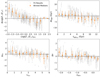 |
Fig. B.1. Residuals (Δ= Fit-Simulation) for the best-fit values for the default (griz) test galaxy fits as a function of the original simulation parameters. From top to bottom and left to right, we have: log(Z⋆/Z⊙), tage, τV and n. Results for the different galaxies are shown in gray. Binned means for each parameter are shown in orange, with error bars given by the standard deviation in each bin. |
Overall, as stated before, the fit shows remarkable quality, considering only four photometric data points were used for each galaxy. There are, however, some accuracy problems present in the fit, especially in the case of the metallicity, as there is a strong bias that skews the recovered values, resulting in a median relative error of 55%. This inaccuracy is particularly noticeable for the extreme values of log(Z⋆/Z⊙). It is possible that this is a byproduct of the difficulty in sourcing accurate spectra with which to build accurate CSP models for nonsolar stellar metallicities (Leja et al. 2017). However, given that the spectra used for both the simulation and the fit are drawn from the same library, it is unlikely this is the root of the observed behavior. This also means that we do not recover the expected mass-metallicity relation in our fitted sample. Although less noticeable, there also seems to exist a slight skew for larger values of tage. These skews are most likely linked to the degeneracy between log(Z⋆/Z⊙) and tage.
To better perceive the quality of these results, we look next to how they compare to the fit results obtained in the same model conditions while using a combined griz + NUV/FUV GALEX + JHKs 2MASS photometry. These results are displayed in Fig. B.2. Although some deviations are observed, on the whole the results appear mostly consistent, reinforcing the previously stated conclusion that a griz photometry fit can adequately determine host dust properties.
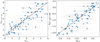 |
Fig. B.2. Comparison between the best-fit values for the simulated test galaxy fits obtained with DECam griz photometry (x-axis) and DECam griz + NUV/FUV GALEX + JHKs 2MASS photometry (y-axis). From left to right we have: τV and n. |
As seen from Table 1, the largest changes to the recovered dust parameters occur when different attenuation models are considered for the simulation and the fits. For the test case where a Cardelli attenuation law was used for the simulations, the differences between the recovered best-fit values and the “true” simulation values are plotted in Fig. B.3. As previously mentioned, RV is the most affected parameter, with a clear bias observed in the recovered values. In addition, there are large errors accompanying these results, which come about due to the conversion between different n and RV.
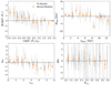 |
Fig. B.3. Residuals (Δ= Fit-Simulation) for the best-fit values for the Cardelli test galaxy fits as a function of the original simulation parameters. From top to bottom and left to right we have: log(Z⋆/Z⊙), tage, τV and n. Results for the different galaxies are shown in gray. Binned means for each parameter are shown in orange, with error bars given by the standard deviation in each bin. |
One final point that should be considered is that, while we have shown that, for the most part, a change in the simulation SFH does not greatly impact the determination of dust properties, there might still be an impact on the age parameter, which might influence the subsequent analysis in Section 4.
To do so, we focus on the fits obtained from the simulations obtained using a delayed-τ model with τ = 10. The comparison between the recovered best-fit values and the “true” simulation values is plotted in Fig. B.4.
 |
Fig. B.4. Residuals (Δ= Fit-Simulation) for the best-fit values for the τ = 10 test galaxy fits as a function of the original simulation parameters. From top to bottom and left to right we have: log(Z⋆/Z⊙), tage, τV and n. Results for the different galaxies are shown in gray. Binned means for each parameter are shown in orange, with error bars given by the standard deviation in each bin. |
It is clear that a discrepancy between the simulation and fit SFHs introduces a great level of bias into the recovered age results. In particular, as the SFH used for the simulation decays more slowly than the SFH presumed in the fitting process, there is a greater amount of star formation at older ages than expected. As such, the fit ends up predicting a younger age for these galaxies. If we instead consider a simulation SFH that decays faster than the one presumed for the fit, then we encounter the opposite problem, with young galaxies appearing much older in the fit. A similar effect happens for simulations with quenched SFHs.
The Spearman correlation coefficients between the simulated and fitted stellar ages for the variable SFH test fits are shown in Table B.1. While there is a degree of correlation prevalent, it starts breaking down as the simulation model moves further away from the default fit model. However, while older galaxies might appear younger and younger galaxies might appear older, an order relation appears to be maintained in the fits. As such, while the specific tage values recovered might be called into question, the broad division of the galaxies into "young" and "old" galaxies can be preserved and relied upon.
Spearman correlation coefficients between the simulated and fitted stellar ages tage for the variable SFH test fits.
Appendix C: Fixed-extinction SN Ia standardization
In this appendix, we discuss the viability of an alternative SN Ia standardization. If the existence of the β color–luminosity relation in Eq. (2) was entirely due to dust, then we would have (e.g., González-Gaitán et al. 2021):
Using this fact, we can separate the extinction βRV and intrinsic βint components in the β color–luminosity relation in Eq. 2, such that (e.g., Brout & Scolnic 2021):
leaving out a possible additional measurement noise term (e.g., Popovic et al. 2021).
It is thus possible to introduce an alternative “Fixed-Extinction” SN Ia standardization in which the values of  and E(B − V) = 1.086(τB − τV) can be fixed using host galaxy measurements. The new nuisance fit parameters are thus α, βint and M. We use the values of RV and E(B − V) obtained in Section 4 from the CSP fits of the SN host galaxies to constrain the color–luminosity relation in the respective “Fixed-Extinction” standardization.
The σ2 in Eq. 3 is thus given by:
where σmB, σx1 and σc are the uncertainties associated with each of the light-curve fit parameters, σmB, c, σmB, x1, σx1, c are their covariance terms, σAB and σE(B − V) are the uncertainties associated with the attenuation law parameters for the host galaxies and σint is a parameter which accounts for possible intrinsic variations in a SN Ia’s luminosity. We fix σint = 0.107, following the value obtained by González-Gaitán et al. (2021).
The cosmological fit parameters obtained for the "Fixed-Extinction" standardization are shown in Table. C.1. This standardization yields RMS values of 0.515 and 0.575 in the global and the local cases, respectively. As previously hinted, both the global and the local measurements produce consistent results. However, judging from the RMS values, the “Fixed-Extinction” standardization appears to be a much worse fit of the data, invalidating it as a replacement for the Tripp standardization, which has a RMS value of 0.141. This is probably due to the fact that, according to Fig. 5, host attenuation laws do not accurately describe SN extinction, meaning it is likely that the problem resides in the values used to approximate SN extinction.
Global and Local fit parameters for the “Fixed-Extinction” and “Fixed-Extinction” + τV bias standardizations and respective RMS
A possible source of error may come from the bias in τV observed in Section 3, which might be skewing the standardization fit results. We can correct for this effect by subtracting the bias level from each τV value. For this, the largest bias value found was used, which was 0.263. For values below the bias threshold, we simply keep the original value. The results obtained from a “Fixed-Extinction” biased standardization are also listed in Table. C.1. The τV bias improves the standardization, with new RMS values of 0.420 and 0.372, for the global and the local cases, respectively. Even so, the bias corrected standardization still falls short of the Tripp values.
On the whole, the proposed “Fixed-Extinction” SN Ia standardization does not provide better fits than standard Tripp standardization. This is most likely a consequence of using host attenuation to approximate SN Ia extinction, as already seen in Section 4.4. However, it is possible that, using extinction data directly obtained for each SN and not its environment, this method might indeed prove to significantly improve cosmological fits and possibly reduce or completely eliminate the mass step.
Appendix D: Cosmological fits with steps
In this appendix, a deeper look at the relation between the mass and dust steps is presented. In particular, for a slightly more robust analysis of both these steps, we can directly introduce δμM and δμD terms in the cosmological fit. We promote the respective step magnitudes γM and γD to free parameters, fixing the step locations to the values previously recovered for the Tripp standardization in Section 5.2.
As mentioned in Section 5.1, the likelihood defined by Eq. 3 can introduce biases into the recovered fit parameters. While this fact is not entirely significant when comparing two standardizations, it becomes important when dealing with a more rigorous cosmological fit. For this reason, when promoting either the mass or dust steps to free fit parameters, it is helpful to slightly modify the likelihood used (e.g., González-Gaitán et al. 2021):
In order to study the various steps, we look at three possible standardizations: a Tripp+mass-step standardization, in which γM is promoted to a free fit parameter; a Tripp+dust-step standardization, in which γD is promoted to a free fit parameter; and a Tripp+mass-step+dust-step standardization, in which both γM and γD are promoted to free fit parameters. It is also useful to redo the standard Tripp standardization to establish a term of comparison for the new likelihood.
For an even more rigorous fit, we can also promote the σint term to a free parameter. Additionally, in the cases where a step is considered, we can assign different σint values to each population. Taking into account both the high and low-mass populations and the regions defined by Fig. 8, we have: Tripp (1 population): full sample (σint1); Tripp + mass step (2 populations): low-mass (σint1), and high-mass (σint2); Tripp + dust step (2 populations): Region 2 (σint1), and Regions 1,3,4 (σint2); Tripp + mass step + dust step (4 populations): low-mass + region 2 (σint1), low-mass + regions 1,3,4 (σint2), high-mass + region 2 (σint3), and high-mass + regions 1,3,4 (σint2).
The recovered fit parameters, as well as the corresponding RMS values, are listed in Table D.1. As expected, the addition of separate mass and dust steps results in lower RMS values, for both the global and the local cases. The dust-step value recovered for the global case is compatible with zero, which might be due to a problem with the fit convergence. The simultaneous inclusion of mass and dust steps produces the lowest values of RMS for the respective cosmological fits. In addition, when both steps are simultaneously included, we recover both noticeable mass and dust steps, with the caveat that the global dust step is once again compatible with zero. In general, the step magnitudes in this case are overall lower than those obtained in the single step cases. As such, we once again find evidence that, although there is some level of overlap, the two steps are not completely analogous and interchangeable.
Fit parameters for the Tripp, Tripp+δμM, Tripp+δμD and Tripp+δμM+δμD standardizations and respective RMS.
Appendix E: Host galaxy fit results
Best-fit results for the DES host galaxy fits with DECam griz global and local photometry.
All Tables
Precision and accuracy metrics for the dust parameters in the mock galaxy fits, for each of the test sets.
Median global and local RV values, standard deviations (STD) and standard errors (SE) for low- and high-mass galaxies.
Spearman correlation coefficients between the global and the local host galaxy attenuation parameters and the respective SN Ia light-curve parameters.
Mass-step significance (in σ), magnitude (γM), ΔRMS and RMSdual for the Tripp and Tripp+δμD standardizations.
Dust-step significance (in σ), magnitude (γD), ΔRMS and RMSdual for the Tripp and Tripp+δμM standardizations.
Mass-step significance (in σ), magnitude (γM), ΔRMS and RMSdual for different color populations.
Dust-step significance (in σ), magnitude (γD), ΔRMS and RMSdual for different color populations.
Spearman correlation coefficients between the simulated and fitted stellar ages tage for the variable SFH test fits.
Global and Local fit parameters for the “Fixed-Extinction” and “Fixed-Extinction” + τV bias standardizations and respective RMS
Fit parameters for the Tripp, Tripp+δμM, Tripp+δμD and Tripp+δμM+δμD standardizations and respective RMS.
Best-fit results for the DES host galaxy fits with DECam griz global and local photometry.
All Figures
|
Fig. 1. Best-fit values of n as a function of τV for the fitted DES galaxies with DECam global (left panel) and local (right panel) griz photometry. Results for the different galaxies are shown in gray. A Gaussian Process Regression is shown in solid blue, with dashed blue lines defining a 68% credible interval. The mean relation found for similar simulated galaxies by Chevallard et al. (2013) is shown in dashed orange, with ±25% error margins shown in dotted orange. |
| In the text | |
|
Fig. 2. Differences (Δ= Global-Local) between best-fit results for the parameters obtained with global and local DECam griz photometry for the DES galaxies, as a function of z. The left-hand side shows the results for τV and the right-hand side the ones for n. Results for the different galaxies are shown in gray. Binned means for each parameter are shown in orange, with error bars given by the standard deviation in each bin. |
| In the text | |
|
Fig. 3. Schematic representation of dust attenuation for different galaxy orientations: Head-on (left panel) and Edge-on (right Panel). |
| In the text | |
|
Fig. 4. Best-fit results for the dust parameters as a function of log(M⋆/M⊙) for the fitted DES galaxies with DECam global (left panels) and local (right panels) griz photometry. Plots for τV are shown in the top row, while results for n are shown in the bottom row. The best-fit for the age of each galaxy is plotted on a gradient from blue (younger) to red (older). |
| In the text | |
|
Fig. 5. Best-fit values of RV as a function of τV for the fitted DES galaxies with DECam Global (left panel) and Local (right panel) griz photometry. Results for the different galaxies are shown in gray. A Gaussian Process Regression is shown in solid blue, with dashed blue lines defining a 68% credible interval. The correlation found by Mandel et al. (2011) between these two quantities for the extinction laws of a set of nearby SNe Ia is shown in orange. |
| In the text | |
|
Fig. 6. Variation of the mass step with step location for the Tripp standardization, for the global (left panels) and the local (right panels) cases. The top panel shows the significance of the step in σ, the middle panel shows the magnitude of the step in solid black, with the gray region showing the uncertainty, and the lower panel shows ΔRMS. In these three panels, the location of the step of maximum significance is shown in blue and the median mass of the sample is shown in orange. Inspired by Kelsey et al. (2021). |
| In the text | |
|
Fig. 7. Hubble residuals Δμ for the DES SNe Ia as a function of the stellar mass for the respective host galaxies, plotted in gray. The optimal step locations, as recorded in Table 5 are shown in dashed blue. The blue dots show the mean values of log(M⋆/M⊙) and Δμ in each bin, with the error in the x-axis given by the standard deviation. |
| In the text | |
|
Fig. 8. Schematic representations of the regions singled out by each of the proposed dust-step splits in the τV − n parameter space. The best-fit values of n as a function of τV for the fitted DES galaxies with global griz photometry are shown for reference. The dashed lines only represent possible division points for the populations, with the actual optimal values recorded in in Table 6. |
| In the text | |
|
Fig. 9. Variation of the Second Split dust step with the step location (position in τV − n grid) for the Tripp standardization. Results from global measurements are shown on the left, while those from local measurements are shown on the right. The top panel shows the significance of the step in σ, the middle panel shows the magnitude of the step and the lower panel shows ΔRMS. This last quantity is defined as the difference between the RMSsingle obtained for a single population mean description and the RMSdual obtained for a dual population mean description with a step. |
| In the text | |
|
Fig. 10. Best-fit values of n as a function of τV for the fitted DES galaxies with DECam global (left panel) and local (right panel) griz photometry. The corresponding value of log(M⋆/M⊙) is plotted on a gradient from blue (lower mass) to red (higher mass). The optimal step for the Second Split is also shown in purple. |
| In the text | |
|
Fig. A.1. Comparison between the stellar mass values obtained by Kelsey et al. (2021) for the host galaxies of the DES-SN sample and the masses recovered using a five-parameter sampling with no initial minimization. In both cases, fits were performed using global (Left panel) and local (Right panel) DECam griz photometry. The results are shown in blue. A dashed line with y = x is also shown. |
| In the text | |
|
Fig. B.1. Residuals (Δ= Fit-Simulation) for the best-fit values for the default (griz) test galaxy fits as a function of the original simulation parameters. From top to bottom and left to right, we have: log(Z⋆/Z⊙), tage, τV and n. Results for the different galaxies are shown in gray. Binned means for each parameter are shown in orange, with error bars given by the standard deviation in each bin. |
| In the text | |
|
Fig. B.2. Comparison between the best-fit values for the simulated test galaxy fits obtained with DECam griz photometry (x-axis) and DECam griz + NUV/FUV GALEX + JHKs 2MASS photometry (y-axis). From left to right we have: τV and n. |
| In the text | |
|
Fig. B.3. Residuals (Δ= Fit-Simulation) for the best-fit values for the Cardelli test galaxy fits as a function of the original simulation parameters. From top to bottom and left to right we have: log(Z⋆/Z⊙), tage, τV and n. Results for the different galaxies are shown in gray. Binned means for each parameter are shown in orange, with error bars given by the standard deviation in each bin. |
| In the text | |
|
Fig. B.4. Residuals (Δ= Fit-Simulation) for the best-fit values for the τ = 10 test galaxy fits as a function of the original simulation parameters. From top to bottom and left to right we have: log(Z⋆/Z⊙), tage, τV and n. Results for the different galaxies are shown in gray. Binned means for each parameter are shown in orange, with error bars given by the standard deviation in each bin. |
| In the text | |
Current usage metrics show cumulative count of Article Views (full-text article views including HTML views, PDF and ePub downloads, according to the available data) and Abstracts Views on Vision4Press platform.
Data correspond to usage on the plateform after 2015. The current usage metrics is available 48-96 hours after online publication and is updated daily on week days.
Initial download of the metrics may take a while.