| Issue |
A&A
Volume 676, August 2023
|
|
|---|---|---|
| Article Number | A49 | |
| Number of page(s) | 15 | |
| Section | Extragalactic astronomy | |
| DOI | https://doi.org/10.1051/0004-6361/202346364 | |
| Published online | 07 August 2023 | |
X-ray properties and obscured fraction of AGN in the J1030 Chandra field⋆
1
Dipartimento di Fisica e Astronomia, Università di Firenze, via G. Sansone 1, 50019 Sesto Fiorentino, Firenze, Italy
e-mail: matilde.signorini@unifi.it
2
INAF – Osservatorio Astrofisico di Arcetri, Largo Enrico Fermi 5, 50125 Firenze, Italy
3
University of California-Los Angeles, Department of Physics and Astronomy, 430 Portola Plaza, Los Angeles, CA 90095-1547, USA
4
INAF – Osservatorio di Astrofisica e Scienza dello Spazio di Bologna, Via Piero Gobetti, 93/3, 40129 Bologna, Italy
5
Department of Physics and Astronomy, Clemson University, Kinard Lab of Physics, Clemson, SC 29634, USA
6
Dipartimento di Fisica e Astronomia, Università degli Studi di Bologna, via Gobetti 93/2, 40129 Bologna, Italy
7
Department of Physics, University of Miami, Coral Gables, FL 33124, USA
8
Institut de Ciéncies del Cosmos (ICCUB), Universitat de Barcelona (IEEC-UB), Martí i Franqués 1, 08028 Barcelona, Spain
9
ICREA, Pg. Luís Companys 23, 08010 Barcelona, Spain
10
Space Telescope Science Institute, 3700 San Martin Drive, Baltimore, MD 21218, USA
11
Scuola Internazionale Superiore di Studi Avanzati (SISSA), Via Bonomea 265, 34136 Trieste, Italy
12
Istituto di Radioastronomia (IRA), Via Piero Gobetti 101, 40129 Bologna, Italy
Received:
9
March
2023
Accepted:
17
May
2023
The 500ks Chandra ACIS-I observation of the field around the z = 6.31 quasar SDSS J1030+0524 is currently the fifth deepest extragalactic X-ray survey. The rich multi-band coverage of the field allowed an effective identification and redshift determination of the X-ray source counterparts; to date, a catalog of 243 extragalactic X-ray sources with either a spectroscopic or photometric redshift estimate in the range z ≈ 0 − 6 is available over an area of 355 arcmin2. Given its depth and the multi-band information, this catalog is an excellent resource to investigate X-ray spectral properties of distant active galactic nuclei (AGN) and derive the redshift evolution of their obscuration. We performed a thorough X-ray spectral analysis for each object in the sample, and measured its nuclear column density NH and intrinsic (de-absorbed) 2–10 keV rest-frame luminosity, L2 − 10. Whenever possible, we also used the presence of the Fe Kα emission line to improve the photometric redshift estimates. We measured the fractions of AGN hidden by column densities in excess of 1022 and 1023 cm−2 (f22 and f23, respectively) as a function of L2 − 10 and redshift, and corrected for selection effects to recover the intrinsic obscured fractions. At z ∼ 1.2, we found f22 ∼ 0.7 − 0.8 and f23 ∼ 0.5 − 0.6, respectively, in broad agreement with the results from other X-ray surveys. No significant variations in X-ray luminosity were found within the limited luminosity range probed by our sample (log L2 − 10 ∼ 42.8 − 44.3). When focusing on luminous AGN with log L2 − 10 ∼ 44 to maximize the sample completeness up to large cosmological distances, we did not observe any significant change in f22 or f23 over the redshift range z ∼ 0.8 − 3. Nonetheless, the obscured fractions we measure are significantly higher than is seen in the local Universe for objects of comparable intrinsic luminosity, pointing toward an increase in the average AGN obscuration toward early cosmic epochs, as also observed in other X-ray surveys. We finally compared our results with recent analytic models that ascribe the greater obscuration observed in AGN at high redshifts to the dense interstellar medium (ISM) of their hosts. When combined with literature measurements, our results favor a scenario in which the total column density of the ISM and the characteristic surface density of its individual clouds both increase toward early cosmic epochs as NH, ISM∝(1 + z)δ, with δ ∼ 3.3 − 4 and Σc, * ∝ (1 + z)2, respectively.
Key words: galaxies: active / X-rays: general / galaxies: high-redshift / quasars: supermassive black holes
Full Table 3 is only available at the CDS via anonymous ftp to cdsarc.cds.unistra.fr (130.79.128.5) or via https://cdsarc.cds.unistra.fr/viz-bin/cat/J/A+A/676/A49
© The Authors 2023
 Open Access article, published by EDP Sciences, under the terms of the Creative Commons Attribution License (https://creativecommons.org/licenses/by/4.0), which permits unrestricted use, distribution, and reproduction in any medium, provided the original work is properly cited.
This article is published in open access under the Subscribe to Open model. Subscribe to A&A to support open access publication.
1. Introduction
The characterization of active galactic nuclei (AGN) demographics and their evolution is crucial to understanding the history of the accretion onto supermassive black holes (SMBHs) and their relation with their host galaxies. We know that the masses of SMBHs residing in the centers of most galaxies correlate with the host properties, such as stellar luminosity, stellar mass, and bulge velocity dispersion (e.g., Marconi & Hunt 2003; Ferrarese et al. 2006; Kormendy & Ho 2013; de Nicola et al. 2019). These correlations indicate a co-evolution scenario of SMBHs and galaxies across cosmic epochs that has been observationally investigated and theoretically modeled (e.g., Croton et al. 2006; Somerville et al. 2008; Fabian 2012; Habouzit et al. 2019; Ricarte et al. 2019), but is still far from being understood in its entirety. For example, in the early Universe the very formation and accretion processes leading to the first SMBHs are still debated. A simple accretion history on stellar mass black holes formed by the first stars is challenged by the discoveries of SMBHs of 1–10 billion solar masses at redshifts higher than 6 (Mortlock et al. 2011; Wu et al. 2015; Bañados et al. 2016; Farina et al. 2022; see also Fan et al. 2022, for a recent review). To match these masses, the accretion process needs to be Eddington-limited or even super-Eddington for long times, or we need to have very massive black hole “seeds” to start with.
Although both the accretion process and the masses of the seeds are still debated, the majority of galaxies are thought to have undergone an active nuclear phase, in which they can be detected as AGN (Kormendy & Ho 2013). This makes investigations of AGN at different cosmic epochs crucial so that we can understand the growth and evolution of both SMBHs and galaxies.
However, the presence of gas and dust, both in the innermost nuclear regions and across the whole host galaxy, poses a significant challenge to AGN detection and characterization, given the damping of the emission in the optical-UV band, where AGN intrinsic power peaks. AGN population synthesis models agree that most SMBH growth is hidden to our view by high gas column densities (see, e.g., Gilli et al. 2007; Ueda et al. 2014; Ananna et al. 2019). This scenario has been confirmed by several observational works (e.g., Lanzuisi et al. 2018; Vito et al. 2018), which further show that, at high redshifts (z > 3–4), the fraction of luminous AGN obscured by column densities NH > 1023 cm−2 is particularly high, ∼80%, as opposed to 20–30% measured in the local Universe (see, e.g., Torres-Albà et al. 2021).
X-ray surveys provide one of the most effective ways to detect obscured AGN over a wide range of redshifts and luminosities (see, e.g., Brandt & Alexander 2015; Xue 2017; Hickox & Alexander 2018, for an extensive review), and are therefore key to finding and characterizing accreting supermassive black holes in the early Universe. While the AGN emission in the X-rays is < 10% of the overall AGN luminosity (e.g., Lusso et al. 2012; Duras et al. 2020), it undergoes very little contamination from non-AGN processes (e.g., X-ray binaries, diffuse gas emission), and is significantly less biased against obscuration than optical emission. These reasons make X-ray surveys a great and efficient way to detect AGN and to characterize them and their obscuration. Several works have used X-ray data to investigate the evolution of AGN obscuration with cosmic times (La Franca et al. 2005; Tozzi et al. 2006; Treister & Urry 2006; Ueda et al. 2014; Buchner et al. 2015; Aird et al. 2015; Liu et al. 2017; Vito et al. 2018; Lanzuisi et al. 2018; Iwasawa et al. 2020; Peca et al. 2023). These works find that the fraction of obscured objects increases with redshift, but the physical origin of this trend is not completely understood (see, e.g., Iwasawa et al. 2012). There are indeed arguments that suggest that the properties of the obscuring torus do not evolve significantly: for example, the spectral energy distributions (SEDs) of AGN are the same at very different redshifts (Richards et al. 2006; Bianchini et al. 2019). This means that the covering factor of the dusty torus is unlikely to change with time. The properties of the interstellar medium (ISM) of the host galaxies, instead, vary significantly with time. The content of gas is higher at early cosmic times (see, e.g., Scoville et al. 2017; Tacconi et al. 2018; Aravena et al. 2020), and galaxies are also smaller in size (Allen et al. 2017; Fujimoto et al. 2017). This means that, as the ISM density increases at high redshift, its column density can reach very high values and be the principal contribution to the obscuration of AGN, as shown in several recent works (e.g., Circosta et al. 2019; D’Amato et al. 2020; Gilli et al. 2022). This has also been shown by hydrodynamic (Trebitsch et al. 2019) and cosmological (Ni et al. 2020) simulations.
In this work we investigate the X-ray properties and derive the obscured fraction of the AGN sample in the J1030 Chandra deep survey. In 2017 Chandra observed a 355 arcmin2 region around the z = 6.31 quasar SDSS J1030+0525 for ∼500 ks. The field around it has dense multi-wavelength coverage, being observed with MUSYC-DEEP, HST/WFC3, HST/ACS, VLT/MUSE, WIRCam, IRAC (see, e.g., Peca et al. 2021). The Chandra survey has a 0.5–2 keV flux limit f0.5 − 2 keV = 6 × 10⁻¹⁷ erg s−1 cm−2 in the central square arcmin and it is, to date, the fifth deepest extragalactic X-ray field (Nanni et al. 2020). The survey resulted in the detection of 256 sources, of which 3 are identified as stars based on their spectra, and 4 more based on their brightness in the K band and low X-ray-to-optical rate (Nanni et al. 2020; Marchesi et al. 2021). Among the remaining 249 extragalactic sources, Marchesi et al. (2021) were able to compute a photo-z for 243 of them, which make the sample considered in this work.
Multiple spectroscopic campaigns allowed the determination of the spectroscopic redshifts for 135 objects out of these 243 (i.e., 56% of the extragalactic sample; Marchesi et al. 2021, 2023). Here we present the complete spectral analysis of the X-ray spectra of the 243 Chandra J1030 extragalactic objects. Our goal is to determine the physical properties of these sources and to study the evolution of the obscured AGN fraction with luminosity and redshift. The paper is structured as follows: in Sect. 2 we describe the X-ray sample and the reduction of the Chandra data; in Sect. 3 we describe the X-ray spectral analysis and its overall results for the sample; in Sect. 4 we derive the obscured AGN fraction in the J1030 Chandra field as a function of luminosity and redshift and for different absorption thresholds; in Sect. 5 we discuss the results, the physical interpretations and the limits of our work, and in Sect. 6 we draw our conclusions. Throughout the rest of the work we assume a flat ΛCDM cosmology with H0 = 69.6 km s−1 Mpc−1, Ωm = 0.29 and ΩΛ = 0.71 (Bennett et al. 2014).
2. Sample description and X-ray spectral extraction
The Chandra J1030 extragalactic sample is made of 243 objects, for which we have a redshift estimate that can be either photometric or spectroscopic. In Fig. 1 we show the redshift distribution of the objects in the catalog; a spectroscopic redshift estimate is available for 135 of them. For 20 out of the 108 photometric estimates, the redshift probability distribution is flat (see Marchesi et al. 2021)1. In Fig. 1 we show their minimum redshift estimate. The 135 objects with spectroscopic redshift also have spectral classification and are divided into four categories (see Marchesi et al. 2021): 20 narrow-line AGN (NL-AGN), 43 broad-line AGN (BL-AGN), 32 early type galaxies (ETG), and 40 emission line galaxies (ELG). The numbers above are updated with respect to the values reported in Marchesi et al. (2021), following new spectroscopic observations (Marchesi et al. 2023).
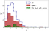 |
Fig. 1. Redshift distribution of the J1030 Chandra catalog. The histograms show the distribution for the whole sample (blue dashed) and the distribution for the objects with spectroscopic redshift (red filled). A spectroscopic redshift is available for 135 out of 243 objects. Also shown is the redshift lower limit for the 20 objects for which the photometric redshift probability distribution is flat (green striped). |
Regarding the objects with only photometric redshift, recent works have proposed a way to derive an additional redshift estimate from the X-ray spectra (e.g., Simmonds et al. 2018; Sicilian et al. 2022). The method was tested for a subsample of the catalog in Peca et al. (2021). However, this method, requires highly obscured objects with a large number of counts (N > 150, Sicilian et al. 2022) to give redshift estimates that are more accurate and reliable than the photometric values. Given the average properties of the sources in our sample, the X-ray spectrum is likely to provide a more precise redshift estimate only when the Fe Kα line is detected. This will be discussed in Sect. 3.
The spectra are extracted using the software Chandra Interactive Analysis of Observations (CIAO) v.4.13. For the choice of the extraction radius, we performed a preliminary ad hoc analysis. We argue that, as the PSF broadens with the increasing of the off-axis angle of the object, the best choice for the extraction radius might be different for objects at different off-axis angles. Furthermore, we expect to include more signal in a larger radius when the signal to noise ratio (S/N) is higher; given this, we might need different radii between low- and high-count objects.
To investigate this issue, we performed an analysis on a randomly chosen subsample of 35 objects that span the off-axis-count plane in the same way as the whole sample. We extracted and fitted the spectra obtained with different extraction radii, corresponding to the 75% 80%, 85%, 90%, and 95% of the encircled energy. We then compared the S/N obtained with each encircled energy choice. The S/N varies significantly between the different choices and, more importantly, there is no clear trend of the maximum of the S/N with the off-axis angle and/or the object counts. Therefore, we deemed an extraction radius R that corresponds to 90% of the encircled energy to be a good choice for all the objects in our sample, consistent with what is already present in the literature (e.g., Marchesi et al. 2016).
For each object, we also extracted a background spectrum in an annulus of radii R+2.5″ and R+20″, manually removing from the annulus any possible contaminating source. The selected background regions provided a sufficient sample for background estimation, allowing the spectral fitting analysis to proceed. For each object, we used the CIAO command specextract to extract the source and the background spectrum and to build the response matrix (RMF) and the ancillary response files (ARFs). This was done for each of the ten observations and the results were then combined with the CIAO tool combine_spectra. To avoid empty channels, the resulting spectra were binned to a minimum of one count per bin. In the end, for each object, we produced the combined source spectrum, the combined background spectrum, and the combined RMF and ARF files.
3. Spectral analysis
Once the spectra and the ancillary files were derived, we fitted them using sherpa (Freeman et al. 2001), fitting the background together with the source. We discuss the background fitting procedure further in Appendix A.
The source spectral shape is modeled with an absorbed power law. The Galactic absorption (NH, Gal = 2.5 × 1020 cm−2) and the redshift are fixed parameters, while the column density at the source redshift, NH, is always assumed to be a free parameter. In principle, the power-law photon index Γ should also be left free to vary. However, given the well-known degeneracy between Γ and NH, in low-statistic spectra, a fit with both parameters free to vary can lead to unreliable results. For this reason, we decided to fix the photon index Γ and leave the column density NH as the only free parameter in sources with 0.5–7 keV net counts below a given threshold. After some tests, we decided to put the threshold at 150 net counts in the 0.5–7 keV band. In Fig. 2 we show the net counts distribution (in the 0.5–7 keV band) for the objects in the catalog. Given the Poissonian nature of the data, we used the C statistic to perform the fit (Cash 1979).
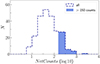 |
Fig. 2. Count histogram for the J1030 field Chandra catalog. There are 39 out of 243 objects that have more than 150 net counts in the 0.5–7 keV range, shown as the light blue filled part of the histogram. |
We first performed the fit procedure for the 39 objects with more than 150 counts. In Fig. 3 we show the resulting photon index distribution; when fitted as a Gaussian, we found ⟨Γ⟩ = 1.89 and a standard deviation σΓ = 0.36. So we assume Γ = 1.9 as a fixed parameter in fitting the objects with less than 150 counts. This value is also consistent with average values of the photon index Γ found in the literature (Mainieri et al. 2007; Lanzuisi et al. 2013; Marchesi et al. 2016; Liu et al. 2017). The free parameters of the fit are then three (the power-law slope, the normalization, and the column density) when the objects have more than 150 counts, and two (the power-law normalization and the column density) otherwise. We derived 90% uncertainties on the fitted parameters with sherpa get_conf(). In Fig. 4 we show four representative X-ray spectra in our sample. For 131 objects out of 243 the fit procedure returned only upper limits for the column density NH; for the others, we obtained NH estimates with upper and lower bounds. We note that an absorbed power-law model may not be an accurate representation of the X-ray spectra of the most heavily obscured, Compton-thick AGN (NH > 1024 cm−2), where reflection components may dominate over the transmitted ones (Comastri et al. 2010; Marchesi et al. 2018). Nonetheless, the primary objective of this study is to determine the fraction of obscured AGN using absorption thresholds of 1022 or 1023 cm−2. In this regard, we contend that an absorbed power-law model is well suited for discerning whether the obscuration of an object exceeds the aforementioned thresholds.
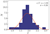 |
Fig. 3. Photon index distribution for the 39 objects with more than 150 net counts. A Gaussian fit gives ⟨Γ⟩ = 1.89, σ = 0.36. |
The Fe Kα line at 6.4 keV is a common feature of X-ray AGN spectra; the more obscured an object is, the more prominent this feature becomes, given the suppression of the primary continuum. Therefore, we expect to find it in a fraction of objects. To check for this presence, we performed the spectral fitting again, adding a new component to the source model, to search for the presence of a line at 6.4 keV. We applied one of two different strategies depending on whether the source has a spectroscopic redshift determination or a photometric one.
For objects with spectroscopic redshifts, we performed a new fit with the same model as before but with the addition of a single Gaussian line with 0.05 keV width. We considered the presence of the line to be significant when compared to the statistic of the best-fitting simple absorbed power-law model; we obtain ΔC > 2.7 as we are adding one free parameter to the fit, the line normalization. This corresponds to a 90% confidence level for one parameter of interest (see, e.g., Avni 1976; Tozzi et al. 2006; Brightman et al. 2014). This happens for 9 objects out of 135: XID 2, XID 4, XID 8, XID 31, XID 44, XID 70, XID 73, XID 114, XID 115. For these objects, we also derived the rest-frame equivalent width of the Fe Kα line. The results are shown in Table 1.
Best-fit parameters for the nine objects with spectroscopic redshifts where a significant Fe Kα line is detected at 6.4 keV.
For objects for which we only have a photometric redshift estimate, the uncertainties on the redshift value are much bigger. Therefore, in searching for a significant Fe Kα line, we let the redshift of the model be a free parameter. We performed the fit with a single power-law model with the addition of a single Gaussian line with a fixed 6.4 keV energy and a fixed 0.05 keV width, imposing the line redshift to be the same as the absorbed power-law. In this case, there are two additional parameters to the fit, which are the redshift and the line normalization. Therefore, we consider the presence of the emission line significant if the difference in the statistic is ΔC > 5.4. We found this to be true for 7 objects: XID 46, XID 137, XID 167, XID 193, XID 200, XID 205, and XID 345, whose properties are shown in Table 2. From this fit, we derive a redshift estimate, which in all cases is consistent with the photometric one, but provides a much smaller uncertainty. The average uncertainty on the redshift estimate for these objects goes from 0.94 in the photometric case to 0.07. We note that for the object XID 205, which has a photometric redshift estimate of  , we get an X-ray redshift estimate of
  , which is consistent with the redshift of the large-scale structure discovered in the field, z = 2.78 (Marchesi et al. 2023).
Often a double power-law component is needed to fit AGN X-ray spectra, to model scattered emission which is typically found in obscured sources (Ueda et al. 2007). To test for the presence of this component, we assumed a phenomenological model and we performed again the fit adding a power-law component with the same photon index as the main one, with no absorption and with a multiplicative constant whose maximum value was fixed at 0.3. Therefore, we only have one additional parameter, the multiplicative constant. We looked for objects for which ΔC > 2.7 but we found none. This differs from the results in previous studies, where at least a few percent of objects are usually found to have a significant double power-law component (e.g., Marchesi et al. 2016).
This might be caused by the decrease in the effective area of the Chandra telescope at energies below ∼1.5 keV, mostly caused by the deposition of materials on the Advanced CCD Imager Spectrometer (ACIS) detector.
3.1. Column density probability distributions
From the spectral fit, we obtain for each object a NH estimate; for 131 out of 243 objects, the estimate is an upper limit for the NH value, while for the others we have a best-fit NH value with upper and lower bounds. We can better understand the NH estimates by deriving the NH probability distributions for the objects in our sample. We used the sherpa command int_proj to compute the fit statistic C as the NH parameter is varied from 1019 to 1026 cm−2, using a logarithmic step of Δlog(NH) = 0.07. Given the statistic values, we derived the probability distribution p(log(NH)∝exp(−C/2)) and normalized its integral to one. In Fig. 5 we show, as an example, the NH probability distributions of the objects shown in Fig. 4. For XID 54 and XID 77, the fitting procedure returns an upper limit for the NH estimate. However, we can see that the probability distributions are very different: for XID 54, each NH value below ∼1022 cm−2 is more or less equally likely; instead for XID 77 and XID 116, there is a clear peak of the probability distribution around ∼3 × 1022 cm−2, although the fit was not able to retrieve a lower bound to the NH estimate. This is true for more than half of the objects in the sample. The NH probability distributions are in many cases asymmetric, with low NH values having a higher probability even when the peak of the distribution is at high NH values. Instead, XID 1892 presents a case in which the best-fitting NH is well constrained, with a 90% lower limit higher than zero. The fit in this case is indeed able to retrieve both an upper and a lower bound for NH. As can be seen with these examples, the probability distribution is a more accurate way to describe the column density of a source, compared with the nominal NH value that we obtain from the fit. We therefore chose to use the p(log(NH)) to derive the obscured fractions, as we discuss in Sect. 4. The NH probability distributions for all the objects in the sample are available on the project webpage3.
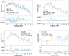 |
Fig. 4. X-ray spectra in the 0.5–7 keV energy range (blue points) and best-fit models (orange solid lines) for four representative objects in the sample. In the lower panel, residuals are shown. The obscuration levels range from unobscured to heavily obscured. The lower panels show the residuals (data-model) of the fit. |
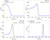 |
Fig. 5. NH probability distributions for the four objects shown in Fig. 4. The yellow dashed lines show the values of NH at which the minimum of the fit statistic is found. For the two objects in the upper panels, we could only derive upper limits to the NH measurements, whereas for the two objects in the lower panels, a significant (> 90% c.l.) column density was measured. |
3.2. Results
At the end of our spectral analysis, we derived the column density NH for the 243 AGN in the J1030 Chandra field. The catalog with the basic physical properties derived from our analysis is available online;4 in Table 3 we show a portion of it. For each object, we provide the column density, the photon index, the (de-absorbed) rest-frame 2–10 keV luminosity, and relative 90% uncertainties. In Fig. 6 we show the global NH-redshift distribution for the sample; the objects are shown with different symbols and colors depending on their spectral identification (Marchesi et al. 2021). A trend of NH with redshift can be seen: objects at higher redshift have on average higher NH values. This is partly due to a selection effect. When moving toward higher redshifts, the photoelectric absorption cutoff moves outside the limit of the observing band, and it is therefore more difficult to constrain lower NH values (Civano et al. 2005; Lanzuisi et al. 2013). A thorough analysis of the obscured fraction trend with redshift that takes this factor into account is provided in the next section.
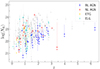 |
Fig. 6. NH-redshift distribution of all the objects in the catalog. Up- and right-pointing arrows show the redshift and NH lower limits for objects with a flat photometric redshift probability curve. Upper limits are shown as down-pointing triangles. The spectral types are color-coded: red, NL-AGN, blue, BL-AGN, yellow, Early Type Galaxies, aquamarine, Emission Line Galaxies, gray, no spectral identification |
Chandra J1030 spectral catalog.
It should be noted that the column densities we obtain for objects for which we have a classification from the optical spectrum are consistent with the optical classifications themselves: BL-AGN (in blue) have low column densities, and for 90% of them the spectral fit can only obtain an upper limit for NH, while NL-AGN (in red) have higher average column densities and the fraction for which we get upper limit for NH is 40%. This fraction is 51% for ELGs and 52% for ETGs. The sources for which we obtain the higher NH values are more likely to be those without an optical spectral classification (in gray), which is consistent with them being obscured and therefore not easily observed in the UV-optical. In Fig. 7 we show the intrinsic (i.e de-absorbed) rest-frame 2–10 keV luminosity versus redshift, with the same classification code.
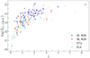 |
Fig. 7. Distribution of the intrinsic (de-absorbed) rest frame 2–10 keV luminosity for the 243 objects in the catalog. Up- and right-pointing triangles show the redshift and luminosity lower limits for objects with a flat photometric redshift probability curve. The color-coding for the spectral types is the same as in Fig. 6. |
4. Obscured fraction
Our goal here is to investigate the dependence of the column density NH on redshift and luminosity. We have to consider that at different redshifts we sample different average luminosities. In the literature there is evidence of the obscuring fraction being a function of both redshift and luminosity (see, e.g., Ueda et al. 2014; Aird et al. 2015; Ananna et al. 2019). Therefore, we need to perform our analysis at a fixed luminosity to derive the evolution of NH with redshift, and at a fixed redshift to derive the NH dependence on luminosity. We considered the intrinsic luminosity-redshift plane, which can be seen in Fig. 8, and we selected only the objects that have a hard band detection, which is 203 out of 243, to get a uniform selection function and to apply reliable correction to go from observed to intrinsic obscured fractions (see Sect. 4.1).
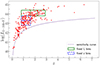 |
Fig. 8. Intrinsic rest-frame 2–10 keV luminosity as a function of redshift for the 203 Chandra J1030 sources detected in the 2–7 keV band. Up- and right- pointing triangles show the redshift and luminosity lower limits for objects with a flat photometric redshift probability curve. The subsample used for the analysis of the NH-redshift evolution (Sect. 4.2) is in green; the subsample used for the analysis of the NH-luminosity evolution (Sect. 4.1) is in blue. The dashed purple line represents the survey sensitivity curve, at 50% of the field coverage (Nanni et al. 2020). |
For the luminosity-dependence analysis, we selected the subsample shown in blue, where the average redshift is ∼1.2 in each bin. This subsample can be divided into three luminosity bins, with 42.8 < log(L2 − 10 keV) < 43.3, 43.3 < log(L2 − 10 keV) < 43.8, and 43.8 < log(L2 − 10 keV) < 44.5, respectively. In each bin, we have 38, 32, and 18 objects, respectively. Of these objects, the ones with a spectroscopic redshift estimate are 19 out of 38 in the first bin, 11 out of 32 in the second bin, and 11 out of 18 in the third bin.
For the redshift dependence analysis, we selected a subsample of objects, shown in green, with an average luminosity of 1044 erg s−1. This subsample is then divided into three subsamples with redshift 0.8 < z < 1.6, 1.6 < z < 2.2, and 2.2 < z < 2.8. In each redshift bin, the average luminosity is ∼1044 erg s−1, and we have 18, 24, and 20 objects per bin, respectively. Out of these objects, the ones with a spectroscopic redshift estimate are 11 out of 18 in the first bin, 11 out of 24 in the second bin, and 14 out of 20 in the third bin.
These bins were selected to maximize the source statistics, while keeping the best completeness in each bin. We note that for the few objects with a flat redshift probability distribution (4 out of a total of 60 objects in the five different bins), we used their best redshift estimate to determine whether they belong to a certain bin.
4.1. Obscured fraction dependence on 2–10 keV luminosity
We want to derive the obscured fraction f22 (the fraction of objects with a column density NH > 1022 cm−2) and f23 (the fraction of objects with a column density NH > 1023 cm−2). For each object, we could simply use the best-fit value of NH as the NH estimate. However, this does not take into account how likely it is for the true NH value for a given object to be that of the nominal result of the fit. Furthermore, for objects with similar NH values (or upper limits), the probability distributions can vary significantly from one object to another, as shown before.
Considering all of this, we derived the obscured fractions using the probability distribution functions described in Sect. 3. For each object, we considered the fraction of p(log(NH)) at NH values higher than 1022 cm−2 (1023 cm−2). We summed all the fractions for the objects in a given luminosity bin and got an estimate of the number of obscured sources that correctly takes into account the probability distribution functions. By dividing this number by the total number of objects in the bin, we obtain the observed obscured fraction. We performed this for the two different obscuration thresholds (1022 cm−2 and 1023 cm−2) and for each luminosity bin.
In Fig. 9 we show the comparison between the results obtained via this procedure, which uses the p(log(NH)), and using the nominal values of NH. It can be seen that using the p(log(NH)) we get obscured fractions f that are systematically lower than the others (even by Δf ∼ 0.18). This is expected, as most NH probability distributions are skewed toward lower NH values. Therefore, there are objects for which the nominal NH value can be higher than the obscuration threshold, but that does not overall contribute much to the obscured population in terms of its probability distribution. The asymmetry of the probability distributions mainly depends on the lack of information at soft X-ray energies. Because of this, it is often possible in the fitting procedure to get a high obscuration level excluded, but it is not possible to distinguish between a non-obscured and a mildly obscured object.
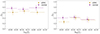 |
Fig. 9. Fraction of obscured z ∼ 1.2 AGN as a function of intrinsic 2–10 keV luminosity. The purple triangles show the observed obscured fractions derived using the nominal NH value derived from the fit. The gold circles are the values obtained using the probability distribution of NH. The second set of points is shifted by 0.05 on the log(L) axis for visual clarity. The 1-σ uncertainties, derived with the bootstrapping procedure, are shown. This figure highlights the relevance of using the probability distributions in deriving the obscured fraction of AGN. These results are still not corrected for the survey sky coverage (for those, see Fig. 11). Left: obscured fraction derived using NH > 1022 cm−2 as the threshold (f22). Right: obscured fraction derived using NH > 1023 cm−2 as the threshold (f23). |
For the uncertainties on these obscured fractions, we know that confidence intervals on sample proportions are usually derived using the binomial distribution. We can, for example, use the Wilson score interval (Wilson 1927) to derive confidence intervals, which will depend, in each bin, on the number of objects in the bin and on the obscured fraction derived using the probability distributions. When doing so for the three luminosity bins, we get lower uncertainties around ∼0.5 and upper uncertainties around ∼0.10. However, this method takes into account the uncertainties related to the finiteness of the sample only and does not consider that the NH estimates are not exact. To deal with this, we derived the uncertainties with a bootstrap procedure: for each bin, we randomly extract, from the bin, with re-entry, a number of objects equal to the bin size. Then, for each object, we extract a value for NH from its probability distribution. We then compute the obscured fraction as the number of objects with NH > 1022 cm−2 over the total. We repeat this 10 000 times and we obtain a f22 (or f23) distribution, from which we extract the peak and the 16% and 84% quantiles as the values for f22 (or f23) and the corresponding uncertainties. In this way, both the finiteness of the bin and the uncertainties on each NH estimate are taken into account.
We now must consider that our survey is flux-limited. This means that we are likely to miss preferentially obscured (i.e. fainter) objects rather than unobscured ones. Therefore, the obscured fractions that we derive are only lower limits to the intrinsic obscured fraction, and the true value is higher. We need to correct the obtained values for the number of objects that we are not observing (called the Malmquist bias). To do so, we proceeded in the following way for each luminosity bin and for each obscuration threshold (1022 and 1023 cm−2): we considered the intrinsic number of obscured and unobscured sources in a given redshift and luminosity range ( and
and  , respectively) expected in the population synthesis model of the cosmic X-ray background (XRB) of Gilli et al. (2007). To derive them, we used the online tool5 to compute the surface density, or integral number counts, N(> S), above any given 2–10 keV flux limit S of both obscured and unobscured AGN. The expected intrinsic number of obscured and unobscured AGN in J1030
  ,
,  were obtained by multiplying the source surface density at f2 − 10 keV = 10−20 cgs (i.e. at ≈ zero flux) by the geometric area of J1030. From the integral number counts, we then obtained the differential source counts dN/dS and folded them with the sky coverage A(S) of the J1030 survey (Nanni et al. 2020) as ∫dn/dSA(S)dS. Because the sky coverage is given in the 2–7 keV flux range, we convert it to the 2–10 keV range by assuming a power-law spectrum with a photon index of 1.4, which is the average observed index for the AGN population.
In this way, we obtain  and
and  , which are the expected observed number of obscured and unobscured objects. We then derived the intrinsic and the observed ratios of the number of obscured objects to unobscured objects,
  and
and  . As we lose more obscured objects than unobscured ones when in the presence of a flux limit, Rint will always be higher than Robs. We can now derive p = Robs/Rint as the corrective parameter that we need to implement to go from our observed obscured fraction to the intrinsic one. This number is always smaller than one.
If we now define the observed obscured fraction(s) as f22 = N[1022 − 1026]/N[1020 − 1026] and f23 = N[1023 − 1026]/N[1020 − 1026], we can derive the corrected fractions as:
and we can derive  in the same way.
We did this for each luminosity bin, starting from the fractions derived with the p(log(NH)), and the resulting corrected fractions are shown in Table 4. In Fig. 10 we show the observed fractions, in dark gold, and the corrected fractions, in orange. We also show the magenta solid line, which is the predicted intrinsic obscured fraction of the Gilli et al. (2007) model, and the dashed purple line which is the observed obscured fraction, given the J1030 X-ray sky coverage. Overall, the high uncertainties make it hard to see a clear trend of the obscured fraction with the luminosity. We can compare our results with others in the literature, with the caveat of only considering those samples of objects with a redshift similar to our (z ∼ 1.2). For the f22 fraction, we can compare it with the work of Aird et al. (2015) (considering the subsample of objects in that work that are found at redshift z ∼ 1), Liu et al. (2017) (considering the objects found at redshift z ∼ 1.2), Iwasawa et al. (2020), and Peca et al. (2023). For the f23 fraction we only have the Liu et al. (2017) data to compare with. These comparisons can be seen in Fig. 11.
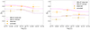 |
Fig. 10. Fraction of z ∼ 1.2 obscured AGN with as a function of intrinsic 2–10 keV luminosity. The gold circles are the observed fraction, while the orange squares are the values obtained once corrected for the survey sky coverage. The second set of points is shifted by 0.05 on the log(L) axis for visual clarity. The solid magenta line represents the predictions from the Gilli et al. (2007) model for the intrinsic obscured fraction; the dashed purple line shows the prediction for the observed fraction accounting for the survey sky coverage. Left: obscured fraction derived using NH > 1022 cm−2 as the threshold (f22). Right: obscured fraction derived using NH > 1023 cm−2 as the threshold (f23). |
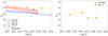 |
Fig. 11. Fraction of z ∼ 1.2 obscured AGN, corrected for completeness, as a function of intrinsic 2–10 keV luminosity. The orange squares show the results from this work. Left: obscured fraction derived using NH > 1022 cm−2 as the threshold (f22). The results from this work are compared with those of Aird et al. (2015, red shaded), Liu et al. (2017, green triangle), Iwasawa et al. (2020, gray star) and Peca et al. (2023, blue shade). The Aird et al. (2015), Iwasawa et al. (2020) and Peca et al. (2023) obscured fraction consider column densities up to 1024 cm−2. Aird et al. (2015) data are centered at z ∼ 1; the Iwasawa et al. (2020) data are centered at z ∼ 1.35. Given the different definitions of f22 and the redshift differences, some scatter among the results is expected. Right: obscured fraction derived using NH > 1023 cm−2 as the threshold (f23). The results of this work are compared with those of Liu et al. (2017, in green). The f23 obscured fraction at log(L)∼44.1 is in good agreement with that of Liu et al. (2017) at log(L)∼43.8. |
Number of objects, average redshift, and fraction of AGN with log(NH) > 22 (f22) and log(NH) > 23 (f23) in three luminosity bin and relative uncertainties.
The f22 that we obtain at log(L)∼44 are consistent with those of Aird et al. (2015) and Liu et al. (2017), while they are higher than those of Iwasawa et al. (2020) and Peca et al. (2023). Overall, the J1030 f22 does not show a significant decline with increasing luminosity as commonly found in the literature, but, given the large error bars, it cannot be ruled out either. For f23, the estimate at log(L)∼44 obtained in this work is consistent with the results of Liu et al. (2017), while we lack data at different luminosities for an additional comparison. We also note that our obscured fractions at z ∼ 1.2 are on average higher than those measured by Aird et al. (2015), Iwasawa et al. (2020) and Peca et al. (2023), as expected: in these works the obscured fraction is derived as the number of objects with 1022 cm−2 < NH < 1024 cm−2 over the number of objects with 1020 cm−2 < NH < 1024 cm−2, while we considered the probability distributions of NH from 1022 cm−2 to 1026 cm−2, that is, we included a correction for an additional population of C-thick AGN.
4.2. Obscured fraction dependence on with redshift
To investigate the redshift evolution of the obscured fraction, we performed the same analysis as described in Sect. 4.1, but for the three redshift bins with the same average luminosity of log(L)∼44 (see Fig. 8). We used the bootstrap procedure to derive, for each bin, the f22 and f23 and the corresponding uncertainties.
We then corrected the observed obscured fractions and recovered the intrinsic ones in each redshift bin using the same correction method described in Sect. 4.1. In Table 5 we show the results of the corrected obscured fractions and their uncertainties in the three redshift bins. The results are shown in Fig. 12. As in Sect. 4.1, we note that, as expected, the corrected fractions are higher than the observed ones, because the presence of a flux limit preferentially removes obscured sources from the sample.
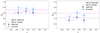 |
Fig. 12. Fractions of log(L2 − 10)∼44 obscured AGN as a function of redshift. The navy circles are the observed fractions, while the light blue squares are those obtained once corrected for the presence of the survey sky coverage. The second set of points is shifted by 0.05 on the z-axis for visual clarity. The solid magenta line represents the predictions from the Gilli et al. (2007) model for the intrinsic obscured fraction; the dashed purple line is the prediction for the observed fraction once the sky coverage is taken into account. Left: obscured fraction derived using NH > 1022 cm−2 as the threshold (f22). Right: obscured fraction derived using NH > 1023 cm−2 as the threshold (f23). |
Number of objects, average 2–10 keV luminosity, and fraction of AGN with log(NH) > 22 (f22) and log(NH) > 23 (f23), corrected for the completeness of the survey, in three redshift bin and relative uncertainties.
We can now compare our results with those of other works. It is important to note that we should compare our obscured fractions with others obtained from samples with similar average luminosity. In Fig. 13 we show our results (in light blue) together with those of Burlon et al. (2011), Aird et al. (2015), Liu et al. (2017), Vito et al. (2018), Iwasawa et al. (2020), and Peca et al. (2023), which are a representative sample of the trends in the literature. The obscured fractions in Liu et al. (2017) were obtained in redshift ranges similar to those used in this study; the results are very consistent for the first two redshift bins, while they are more distant for the higher redshift points. The number of objects per bin in Liu et al. (2017) is roughly the same as in the J1030 sample; our uncertainties of the obscured fraction estimates are significantly higher, given the lower quality of the data and given that we took both the binomial error and the NH uncertainties into account.
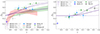 |
Fig. 13. Fraction of log(L)∼44 obscured AGN with NH > 1022 cm−2 (f22) as a function of redshift. The light blue squares show the results from this work. The prediction of the Gilli et al. (2022) model for the evolution of the obscured fraction with the redshift is shown as the indigo lines, with different styles representing the different parameters of the model (see Sect. 5.2). Left: obscured fraction derived using NH > 1022 cm−2 as the threshold (f22). The results from this work are compared with those of Burlon et al. (2011, blue diamond), Liu et al. (2017, green triangle), Aird et al. (2015, red shaded), Iwasawa et al. (2020, gray star), and Peca et al. (2023, green shaded). The Aird et al. (2015), Liu et al. (2017), Iwasawa et al. (2020), and Peca et al. (2023) obscured fraction consider column densities up to 1024 cm−2. Right: obscured fraction derived using NH > 1023 cm−2 as the threshold (f23). The results from work are compared with those of Burlon et al. (2011, blue diamond), Liu et al. (2017, green triangle), and Vito et al. (2018, black pentagon). The Vito et al. (2018) obscured fraction consider column densities up to 1025 cm−2. |
It should be noted that that Aird et al. (2015), Iwasawa et al. (2020), and Peca et al. (2023) obscured fractions consider column densities up to 1024 cm−2. Given the different definitions of f22 and the redshift differences, some discrepancy between the results is expected. When also considering the low-redshift results of Burlon et al. (2011), and the high-redshift Vito et al. (2018) estimate for f23, there is evidence of a clear redshift trend, with bins at higher redshift showing a higher obscured fraction, both for f22 and f23. Overall, our results are consistent with those in the literature.
5. Discussion
In this section, we discuss the results of our analysis and their interpretation, as well as possible limitations and biases.
5.1. Limitations and biases
The first limitation affecting our work is related to the sample statistics. Although the J1030 Chandra survey is one of the deepest X-ray surveys, about 30% of the objects have less than 30 net counts, which affects our ability to derive accurate parameters from the spectral fit. Furthermore, the progressive degradation of the Chandra detectors affects the soft X-ray response in a non-negligible way. As the spectral shape at low energies is more informative and allows us to distinguish between different levels of obscuration, our ability to derive reliable NH estimates is reduced. The low sensitivity at low energies also significantly skews the NH probability distributions toward low NH values, even when a significant probability peak around a certain value is found (see e.g., XID 77 and XID 116 in Fig. 4). These uncertainties clearly affect the accuracy with which we can estimate the obscured AGN fractions, compared with surveys with longer exposures and with surveys where observations have been carried out in earlier years of the Chandra satellite life.
Another source of uncertainty comes from the fact that 44% of the objects in our sample only have a photometric redshift estimate. In the fit procedure, we considered the redshift as a fixed parameter. However, the errors on the photometric redshifts can be significant. This again affects the accuracy of the NH estimates. Furthermore, in the obscured AGN fraction analysis, some objects that fall in a given luminosity-redshift bin might actually belong to other, adjacent bins. Observational campaigns aimed at improving the spectroscopic redshift completeness of the J1030 Chandra sample are being planned.
We measured the obscured AGN fractions in different bins of X-ray luminosity and redshift. The main source of errors on these fractions is related to (i) the limited sample statistics in each luminosity-redshift bin, and (ii) the uncertainties in the column density estimate of each source. Given that the uncertainties we derive from the Wilson score values are in the ∼0.05–0.10 range, compared to total uncertainties derived from the bootstrapping procedure of ∼0.11, we can say that the first contribution is generally more significant than the second. When compared with the results obtained from other surveys, our uncertainties are significantly higher. This depends on the fact that, in general, previous studies do not take both sources of uncertainties into account, on the lower data quality of our X-ray spectra when compared with other samples (e.g., Liu et al. 2017), and on the higher statistics of other surveys.
The uncertainties in our obscured fraction estimates are such that we do not have clear evidence of a redshift or a luminosity trend with the J1030 data alone (see Figs. 11 and 12). At the same time, as shown in Fig. 13, our results are generally consistent with those in the literature for AGN with similar luminosities and at similar redshifts. Furthermore, when combined with samples of X-ray selected AGN covering a broader range of redshifts, our results follow the general literature trends, where the obscured AGN fraction increases toward higher redshifts.
Another bias that might be affecting our results is the classification bias. When an object has a small number of counts, heavily obscured objects can be misclassified as mildly obscured ones (for more details, see Brightman & Ueda 2012; Lanzuisi et al. 2018). The low-luminosity objects are the ones with a smaller number of counts, and therefore the most affected by this bias. In terms of the obscured fraction trend with the luminosity, this means that we are probably underestimating the obscured fraction in the first luminosity bin, which might be preventing us from seeing a clear trend.
5.2. Evolution of the obscured AGN fraction
While the decrease in the obscured AGN fraction with luminosity is generally interpreted in the framework of the so-called receding-torus models (Lusso et al. 2013; Ricci et al. 2017), the physics behind the increasing trend of the obscured fraction with redshift is not completely understood.
We compared our results with the model recently proposed in Gilli et al. (2022). In that work, the authors argue that the evolution of the obscured AGN fraction is produced by the increasing density of the ISM in the host galaxies, and give an analytic model for that. In Fig. 13 we show the predictions of the baseline model of Gilli et al. (2022) as the solid indigo lines. The other lines reflect different assumptions in the model parameters that we discuss below. Considering the baseline model, we see that there is a good agreement for f23, while for f22 our values are higher than the prediction, although consistent at a 1.5σ level. Our measurements are generally in better agreement with the model curves than the measurements of Liu et al. (2017), who found larger obscured AGN fractions at z > 2. We recall, however, that the model curves from Gilli et al. (2022) are an example of how the increased ISM density may provide a good representation of the observed trend, but they were not derived through best-fit procedures to any specific dataset. Here we explore the parameter space of that model further, trying to determine, for instance, how the ISM properties should change with redshift to reproduce the steeper trend observed by Liu et al. (2017).
By considering a number of tracers for the total mass and volume of the ISM in galaxy samples at different redshifts, mainly from ALMA, and simple assumptions on the gas density profiles, Gilli et al. (2022) measured the cosmic evolution of the ISM column density toward the nuclei of massive galaxies. This was parameterized as NH, ISM∝(1 + z)δ. They also assumed that the ISM is composed of individual gas clouds with surface densities and radii distributed as a Schechter function and that the characteristic cloud surface density Σc, * may evolve with redshift as (1 + z)γ. The redshift evolution of the ISM-obscured AGN fraction above a given NH, ISM threshold depends on both δ and γ (see Eqs. (40) and (41) in Gilli et al. 2022). Broadly speaking, a rapid increase in the total column density with redshift would imply a correspondingly rapid increase in the obscured AGN fraction. This increase is nonetheless softened if ISM clouds are significantly denser at earlier cosmic epochs as fewer clouds would then be needed to reproduce the same total gas density, reducing in turn the chances that galaxy nuclei are hidden by one of these. The baseline model in Gilli et al. (2022) assumed δ = 3.3, as driven by the results from ALMA observations, and γ = 2, which, when combined with the obscuration from a small-scale component (i.e. the torus) was found to produce f22 and f23 trends in good agreement with the observations. Clearly, the uncertainties on δ and γ are large, as we still have limited knowledge of the overall ISM properties of distant galaxies. In Fig. 13 we show the expected trends for f22 and f23 when first increasing δ and then decreasing γ, leaving all the other model parameters unchanged. A faster increase in the total ISM density with redshift (δ = 4) is needed to explain the steep trend observed by Liu et al. (2017) for f22 and f23 and the large f23 value measured by Vito et al. (2018) at z ∼ 3.6. On the other hand, interestingly, a milder evolution of the characteristic gas surface density of ISM clouds (γ = 1) would only explain the steeper trend in f22, but not in f23, because, below z ∼ 4 − 5 the distribution of cloud surface densities would be rich in clouds with Σc, * > 1022 cm−2, but still short of high-density clouds with Σc, * > 1023 cm−2. It is only at z ∼ 6 and above that Σc, * would increase enough to return significant fractions of very dense clouds.
To summarize, current measurements of the obscured AGN fractions as a function of cosmic time, including ours, are in agreement with an evolving ISM model in which the total gas column density of massive galaxies evolves as fast as NH, ISM∝(1 + z)3.3 − 4, and in which the individual gas clouds become progressively denser toward early epochs [Σc, * ∝ (1 + z)2]. Such a scenario will likely be tested soon with improved accuracy by new ALMA observations.
5.3. Compton-thick AGN
Our work only considers the X-ray spectral fitting as an obscuration diagnostic. This means that, it is likely that we are not able to correctly characterize heavily obscured objects, especially Compton-thick (CT) AGN, which also tend to have a small number of counts. In addition to this, absorption models like the one we used (phabs) do not work well in a very high column density regime. We find eight objects with a nominal NH higher than 1024 cm−2 out of 243, which means that we have a CT fraction of 3.3%. If we consider the p(log(NH)) and sum all the fractions with NH > 1024 cm−2, we get an observed fraction f24 = 3%, close to that we obtained from nominal values. This value is smaller than the ∼8% CT fraction that is found by Liu et al. (2017) for the Chandra Deep Field South. However, in that work, the authors use additional criteria other than the X-ray spectral fitting to determine if a source is Compton thick. In Lanzuisi et al. (2018), instead, where the only diagnostic is again the X-ray spectral analysis, the CT fraction found in the COSMOS Chandra survey was 2.2%, similar to our result.
Based on these previous results, it is therefore likely that if additional multi-band diagnostics were implemented, we would get a larger number of CT objects. Therefore, the CT fraction that we get is to be considered as a lower limit for the intrinsic value.
6. Conclusions
In this work, we analyzed the X-ray spectra of the 243 extragalactic sources of the J1030 Chandra catalog and used the results to derive the obscured fraction of AGN at different redshift and luminosities. Here we outline the main results of our work and future perspectives.
-
We fitted the Chandra X-ray spectra with absorbed power laws, and checked for the presence of the Fe Kα line and a soft excess. We could use spectroscopic redshift information for 44% of the sample, while we relied on photometric redshift estimates for the rest. For 7 objects with a photometric redshift only, we were able to refine the redshift estimate via X-ray spectroscopy. The best-fit spectral parameters derived for the whole sample are available at the J1030 website6.
-
We measured the obscured fractions f22 and f23 (i.e. the fraction of AGN with NH > 1022 cm−2 and 1023 cm−2, respectively) using the full column density probability distributions derived from the spectral fits p(log(NH)). We measured f22 and f23 in three redshift bins (0.8 < z < 1.6, 1.6 < z < 2.2 and 2.2 < z < 2.8) for AGN with log(L)∼44, and in three luminosity bins (42.8 < log(L2 − 10 keV) < 43.3, 43.3 < log(L2 − 10 keV) < 43.8, and 43.8 < log(L2 − 10 keV) < 44.5), for AGN at z ∼ 1.2. We corrected these observed fractions for the sky coverage of the survey and derived accurate measurement errors through a bootstrapping procedure that accounts for both the finite size of the sample and the uncertainties on the NH estimates.
-
We measured average values of f22 ∼ 0.7 − 0.8 and f23 ∼ 0.5 − 0.6. While these average values are in broad agreement with those in other works (Aird et al. 2015; Liu et al. 2017), we did not see clear trends with luminosity or redshift, as opposed to what is often found in the literature. This might, at least partially, depend on residual, uncorrected biases, and/or on the limited dynamical range in luminosity and redshift spanned by our data. Nonetheless, when combined with measurements performed in the local Universe, our data point to an increase in the obscured AGN fractions with redshift, in agreement with other findings.
-
We finally considered predictions from recent analytic models that ascribe the redshift evolution of the obscured AGN fraction to the increased density of the ISM in high-z hosts, which adds significant obscuration to that of the parsec-scale torus (Gilli et al. 2022). When combined with literature measurements, our results favor a scenario in which the total ISM column density grows with redshift as NH, ISM∝(1 + z)3.3 − 4, and in which the characteristic surface density of individual gas clouds in the ISM evolves as Σc, * ∝ (1 + z)2.
To gain a deeper understanding of nuclear obscuration at different cosmic epochs, and as a function of the various AGN physical properties, large object samples are needed, that would go significantly beyond those available from current X-ray probes. What is believed to be the bulk of the AGN population (low-luminosity, possibly obscured objects) is now partly missed at medium-high redshift values, and completely lost beyond redshift z ∼ 6. Next-generation X-ray imaging surveys, such as those proposed with the Survey and Time-domain Astrophysical Research eXplorer (STAR-X7), a Medium Explorer mission selected by NASA for Phase A study, the Advanced X-ray Imaging Satellite (AXIS, Mushotzky et al. 2019; Marchesi et al. 2020), a probe-class mission proposed to NASA, and the L-class mission Athena under scrutiny at ESA (Nandra et al. 2013), would offer new opportunities to detect and characterize highly obscured sources. These observatories are expected to discover a few thousand heavily obscured (NH > 1023 cm−2) AGN at z > 3, shedding light on the overall growth of SMBHs before cosmic noon.
The photometric SED and redshift probability distributions can be found on the website: http://j1030-field.oas.inaf.it/xray_redshift_J1030.html
Which, we note, is also the central object of the protocluster described in Gilli et al. (2019).
Acknowledgments
We thank the referee for their detailed and constructive suggestions. We acknowledge financial contribution from the agreement ASI-INAF n. 2017-14-H.O.
References
- Aird, J., Coil, A. L., Georgakakis, A., et al. 2015, MNRAS, 451, 1892 [Google Scholar]
- Allen, R. J., Kacprzak, G. G., Glazebrook, K., et al. 2017, ApJ, 834, L11 [NASA ADS] [CrossRef] [Google Scholar]
- Ananna, T. T., Treister, E., Urry, C. M., et al. 2019, ApJ, 871, 240 [Google Scholar]
- Aravena, M., Boogaard, L., Gónzalez-López, J., et al. 2020, ApJ, 901, 79 [NASA ADS] [CrossRef] [Google Scholar]
- Avni, Y. 1976, ApJ, 210, 642 [NASA ADS] [CrossRef] [Google Scholar]
- Bañados, E., Venemans, B. P., Decarli, R., et al. 2016, ApJS, 227, 11 [Google Scholar]
- Bennett, C. L., Larson, D., Weiland, J. L., & Hinshaw, G. 2014, ApJ, 794, 135 [Google Scholar]
- Bianchini, F., Fabbian, G., Lapi, A., et al. 2019, ApJ, 871, 136 [CrossRef] [Google Scholar]
- Brandt, W. N., & Alexander, D. M. 2015, A&ARv, 23, 1 [Google Scholar]
- Brightman, M., & Ueda, Y. 2012, MNRAS, 423, 702 [NASA ADS] [CrossRef] [Google Scholar]
- Brightman, M., Nandra, K., Salvato, M., et al. 2014, MNRAS, 443, 1999 [NASA ADS] [CrossRef] [Google Scholar]
- Buchner, J., Georgakakis, A., Nandra, K., et al. 2015, ApJ, 802, 89 [Google Scholar]
- Burlon, D., Ajello, M., Greiner, J., et al. 2011, ApJ, 728, 58 [Google Scholar]
- Cash, W. 1979, ApJ, 228, 939 [Google Scholar]
- Circosta, C., Vignali, C., Gilli, R., et al. 2019, A&A, 623, A172 [NASA ADS] [CrossRef] [EDP Sciences] [Google Scholar]
- Civano, F., Comastri, A., & Brusa, M. 2005, MNRAS, 358, 693 [NASA ADS] [CrossRef] [Google Scholar]
- Comastri, A., Iwasawa, K., Gilli, R., et al. 2010, ApJ, 717, 787 [NASA ADS] [CrossRef] [Google Scholar]
- Croton, D. J., Springel, V., White, S. D. M., et al. 2006, MNRAS, 365, 11 [Google Scholar]
- D’Amato, Q., Gilli, R., Vignali, C., et al. 2020, A&A, 636, A37 [NASA ADS] [CrossRef] [EDP Sciences] [Google Scholar]
- de Nicola, S., Marconi, A., & Longo, G. 2019, MNRAS, 490, 600 [NASA ADS] [CrossRef] [Google Scholar]
- Duras, F., Bongiorno, A., Ricci, F., et al. 2020, A&A, 636, A73 [NASA ADS] [CrossRef] [EDP Sciences] [Google Scholar]
- Fabian, A. 2012, ARA&A, 50, 455 [CrossRef] [Google Scholar]
- Fan, X., Banados, E., & Simcoe, R. A. 2022, ArXiv e-prints [arXiv:2212.06907] [Google Scholar]
- Farina, E. P., Schindler, J.-T., Walter, F., et al. 2022, ApJ, 941, 106 [NASA ADS] [CrossRef] [Google Scholar]
- Ferrarese, L., Côté, P., Dalla Bontà, E., et al. 2006, ApJ, 644, L21 [Google Scholar]
- Fiore, F., Puccetti, S., Grazian, A., et al. 2012, A&A, 537, A16 [NASA ADS] [CrossRef] [EDP Sciences] [Google Scholar]
- Freeman, P., Doe, S., & Siemiginowska, A. 2001, in Astronomical Data Analysis, eds. J.-L. Starck, & F. D. Murtagh, 4477, 76 [NASA ADS] [CrossRef] [Google Scholar]
- Fujimoto, S., Ouchi, M., Shibuya, T., & Nagai, H. 2017, ApJ, 850, 83 [Google Scholar]
- Gilli, R., Comastri, A., & Hasinger, G. 2007, A&A, 463, 79 [NASA ADS] [CrossRef] [EDP Sciences] [Google Scholar]
- Gilli, R., Mignoli, M., Peca, A., et al. 2019, A&A, 632, A26 [NASA ADS] [CrossRef] [EDP Sciences] [Google Scholar]
- Gilli, R., Norman, C., Calura, F., et al. 2022, A&A, 666, A17 [NASA ADS] [CrossRef] [EDP Sciences] [Google Scholar]
- Habouzit, M., Genel, S., Somerville, R. S., et al. 2019, MNRAS, 484, 4413 [CrossRef] [Google Scholar]
- Hickox, R. C., & Alexander, D. M. 2018, ARA&A, 56, 625 [Google Scholar]
- Iwasawa, K., Gilli, R., Vignali, C., et al. 2012, A&A, 546, A84 [NASA ADS] [CrossRef] [EDP Sciences] [Google Scholar]
- Iwasawa, K., Comastri, A., Vignali, C., et al. 2020, A&A, 639, A51 [NASA ADS] [CrossRef] [EDP Sciences] [Google Scholar]
- Kormendy, J., & Ho, L. C. 2013, ARA&A, 51, 511 [Google Scholar]
- La Franca, F., Fiore, F., Comastri, A., et al. 2005, ApJ, 635, 864 [NASA ADS] [CrossRef] [Google Scholar]
- Lanzuisi, G., Civano, F., Elvis, M., et al. 2013, MNRAS, 431, 978 [NASA ADS] [CrossRef] [Google Scholar]
- Lanzuisi, G., Civano, F., Marchesi, S., et al. 2018, MNRAS, 480, 2578 [Google Scholar]
- Liu, T., Tozzi, P., Wang, J., et al. 2017, AJ, 232, 8 [Google Scholar]
- Lusso, E., Comastri, A., Simmons, B. D., et al. 2012, MNRAS, 425, 623 [Google Scholar]
- Lusso, E., Hennawi, J. F., Comastri, A., et al. 2013, ApJ, 777, 86 [Google Scholar]
- Mainieri, V., Hasinger, G., Cappelluti, N., et al. 2007, ApJS, 172, 368 [NASA ADS] [CrossRef] [Google Scholar]
- Marchesi, S., Lanzuisi, G., Civano, F., et al. 2016, ApJ, 830, 100 [Google Scholar]
- Marchesi, S., Ajello, M., Marcotulli, L., et al. 2018, ApJ, 854, 49 [Google Scholar]
- Marchesi, S., Gilli, R., Lanzuisi, G., et al. 2020, A&A, 642, A184 [EDP Sciences] [Google Scholar]
- Marchesi, S., Mignoli, M., Gilli, R., et al. 2021, A&A, 656, A117 [NASA ADS] [CrossRef] [EDP Sciences] [Google Scholar]
- Marchesi, S., Mignoli, M., Gilli, R., et al. 2023, A&A, 673, A97 [NASA ADS] [CrossRef] [EDP Sciences] [Google Scholar]
- Marconi, A., & Hunt, L. K. 2003, ApJ, 589, L21 [Google Scholar]
- Mortlock, D. J., Warren, S. J., Venemans, B. P., et al. 2011, Nature, 474, 616 [Google Scholar]
- Mushotzky, R., Aird, J., Barger, A. J., et al. 2019, BAAS, 51, 107 [Google Scholar]
- Nandra, K., Barret, D., Barcons, X., et al. 2013, ArXiv e-prints [arXiv:1306.2307] [Google Scholar]
- Nanni, R., Gilli, R., Vignali, C., et al. 2018, A&A, 614, A121 [NASA ADS] [CrossRef] [EDP Sciences] [Google Scholar]
- Nanni, R., Gilli, R., Vignali, C., et al. 2020, A&A, 637, A52 [NASA ADS] [CrossRef] [EDP Sciences] [Google Scholar]
- Ni, Y., Di Matteo, T., Gilli, R., et al. 2020, MNRAS, 495, 2135 [NASA ADS] [CrossRef] [Google Scholar]
- Peca, A., Vignali, C., Gilli, R., et al. 2021, AJ, 906, 90 [NASA ADS] [CrossRef] [Google Scholar]
- Peca, A., Cappelluti, N., Urry, C. M., et al. 2023, ApJ, 943, 162 [NASA ADS] [CrossRef] [Google Scholar]
- Ricarte, A., Tremmel, M., Natarajan, P., & Quinn, T. 2019, MNRAS, 489, 802 [NASA ADS] [CrossRef] [Google Scholar]
- Ricci, C., Koss, M., Trakhtenbrot, B., et al. 2017, in The X-ray Universe 2017, eds. J. U. Ness, & S. Migliari, 190 [Google Scholar]
- Richards, G. T., Strauss, M. A., Fan, X., et al. 2006, AJ, 131, 2766 [Google Scholar]
- Scoville, N., Lee, N., Vanden Bout, P., et al. 2017, ApJ, 837, 150 [Google Scholar]
- Sicilian, D., Civano, F., Cappelluti, N., Buchner, J., & Peca, A. 2022, ApJ, 936, 39 [NASA ADS] [CrossRef] [Google Scholar]
- Simmonds, C., Buchner, J., Salvato, M., Hsu, L. T., & Bauer, F. E. 2018, A&A, 618, A66 [NASA ADS] [CrossRef] [EDP Sciences] [Google Scholar]
- Somerville, R. S., Hopkins, P. F., Cox, T. J., Robertson, B. E., & Hernquist, L. 2008, MNRAS, 391, 481 [NASA ADS] [CrossRef] [Google Scholar]
- Tacconi, L. J., Genzel, R., Saintonge, A., et al. 2018, ApJ, 853, 179 [Google Scholar]
- Torres-Albà, N., Marchesi, S., Zhao, X., et al. 2021, ApJ, 922, 252 [CrossRef] [Google Scholar]
- Tozzi, P., Gilli, R., Mainieri, V., et al. 2006, A&A, 451, 457 [NASA ADS] [CrossRef] [EDP Sciences] [Google Scholar]
- Trebitsch, M., Volonteri, M., & Dubois, Y. 2019, MNRAS, 487, 819 [CrossRef] [Google Scholar]
- Treister, E., & Urry, C. M. 2006, ApJ, 652, L79 [NASA ADS] [CrossRef] [Google Scholar]
- Ueda, Y., Eguchi, S., Terashima, Y., et al. 2007, ApJ, 664, L79 [Google Scholar]
- Ueda, Y., Akiyama, M., Hasinger, G., Miyaji, T., & Watson, M. G. 2014, ApJ, 786, 104 [Google Scholar]
- Vito, F., Brandt, W. N., Yang, G., et al. 2018, MNRAS, 473, 2378 [Google Scholar]
- Wilson, E. B. 1927, J. Am. Stat. Assoc., 22, 209 [CrossRef] [Google Scholar]
- Wu, X.-B., Wang, F., Fan, X., et al. 2015, Nature, 518, 512 [Google Scholar]
- Xue, Y. Q. 2017, New A Rev., 79, 59 [NASA ADS] [CrossRef] [Google Scholar]
Appendix A: Fitting procedure of background spectra
In this Appendix we describe our fitting procedure for the background spectra of our objects. In order to have the most reliable estimates of the parameters we want to fit, we decided to simultaneously fit the source and the background.
We extracted local background spectra, but we do not want to model the background locally as (i) we want to minimize dependencies on sharp background variations and (ii) the number of counts in background spectra extracted in small regions around each source can be very small and therefore the parameters uncertainties very high. We therefore want to characterize the whole background and then use the fitted background model to simultaneously fit each source with its local background, adding a background normalization parameter to the source fit to rescale the normalization to that of the local background. We selected three regions, all centered on the center of the field: one circular region of 3 arcmin radius, one annulus with 3 and 6 arcmin radii and an annulus with 6 and 9 arcmin radii. In each region we excluded circular regions of 5 arcsec radius around all the X-ray detected sources. We extracted the spectrum of each region in the energy range 0.8-7 keV, which is the one we use to fit the sources. We modeled each background spectrum with a power-law and four Gaussian lines, following the model used by Fiore et al. (2012) for the Chandra Deep Field South survey. Following the same model, we also tried to (i) add a second power-law component, and (ii) add a thermal component, but both turned out to be non-significant. We therefore excluded these components from the final background shape, which ends up being composed of a power law and four Gaussians.
In Figure A.1 we can see the spectra and the resulting best-fit. Given the best fit parameters of the modeled background, we used them as "frozen" parameters in the source+background fit analysis, only adding a multiplicative constant as a free parameter to re-scale the background spectrum to that of each object.
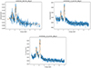 |
Fig. A.1. Spectrum (blue) and best fit (yellow) of the background spectra for different regions of the field: (a) 3’ circle; (b) annulus of radii 3’ and 6’; (c) annulus of radii 6’ and 9’ |
All Tables
Best-fit parameters for the nine objects with spectroscopic redshifts where a significant Fe Kα line is detected at 6.4 keV.
Number of objects, average redshift, and fraction of AGN with log(NH) > 22 (f22) and log(NH) > 23 (f23) in three luminosity bin and relative uncertainties.
Number of objects, average 2–10 keV luminosity, and fraction of AGN with log(NH) > 22 (f22) and log(NH) > 23 (f23), corrected for the completeness of the survey, in three redshift bin and relative uncertainties.
All Figures
|
Fig. 1. Redshift distribution of the J1030 Chandra catalog. The histograms show the distribution for the whole sample (blue dashed) and the distribution for the objects with spectroscopic redshift (red filled). A spectroscopic redshift is available for 135 out of 243 objects. Also shown is the redshift lower limit for the 20 objects for which the photometric redshift probability distribution is flat (green striped). |
| In the text | |
|
Fig. 2. Count histogram for the J1030 field Chandra catalog. There are 39 out of 243 objects that have more than 150 net counts in the 0.5–7 keV range, shown as the light blue filled part of the histogram. |
| In the text | |
|
Fig. 3. Photon index distribution for the 39 objects with more than 150 net counts. A Gaussian fit gives ⟨Γ⟩ = 1.89, σ = 0.36. |
| In the text | |
|
Fig. 4. X-ray spectra in the 0.5–7 keV energy range (blue points) and best-fit models (orange solid lines) for four representative objects in the sample. In the lower panel, residuals are shown. The obscuration levels range from unobscured to heavily obscured. The lower panels show the residuals (data-model) of the fit. |
| In the text | |
|
Fig. 5. NH probability distributions for the four objects shown in Fig. 4. The yellow dashed lines show the values of NH at which the minimum of the fit statistic is found. For the two objects in the upper panels, we could only derive upper limits to the NH measurements, whereas for the two objects in the lower panels, a significant (> 90% c.l.) column density was measured. |
| In the text | |
|
Fig. 6. NH-redshift distribution of all the objects in the catalog. Up- and right-pointing arrows show the redshift and NH lower limits for objects with a flat photometric redshift probability curve. Upper limits are shown as down-pointing triangles. The spectral types are color-coded: red, NL-AGN, blue, BL-AGN, yellow, Early Type Galaxies, aquamarine, Emission Line Galaxies, gray, no spectral identification |
| In the text | |
|
Fig. 7. Distribution of the intrinsic (de-absorbed) rest frame 2–10 keV luminosity for the 243 objects in the catalog. Up- and right-pointing triangles show the redshift and luminosity lower limits for objects with a flat photometric redshift probability curve. The color-coding for the spectral types is the same as in Fig. 6. |
| In the text | |
|
Fig. 8. Intrinsic rest-frame 2–10 keV luminosity as a function of redshift for the 203 Chandra J1030 sources detected in the 2–7 keV band. Up- and right- pointing triangles show the redshift and luminosity lower limits for objects with a flat photometric redshift probability curve. The subsample used for the analysis of the NH-redshift evolution (Sect. 4.2) is in green; the subsample used for the analysis of the NH-luminosity evolution (Sect. 4.1) is in blue. The dashed purple line represents the survey sensitivity curve, at 50% of the field coverage (Nanni et al. 2020). |
| In the text | |
|
Fig. 9. Fraction of obscured z ∼ 1.2 AGN as a function of intrinsic 2–10 keV luminosity. The purple triangles show the observed obscured fractions derived using the nominal NH value derived from the fit. The gold circles are the values obtained using the probability distribution of NH. The second set of points is shifted by 0.05 on the log(L) axis for visual clarity. The 1-σ uncertainties, derived with the bootstrapping procedure, are shown. This figure highlights the relevance of using the probability distributions in deriving the obscured fraction of AGN. These results are still not corrected for the survey sky coverage (for those, see Fig. 11). Left: obscured fraction derived using NH > 1022 cm−2 as the threshold (f22). Right: obscured fraction derived using NH > 1023 cm−2 as the threshold (f23). |
| In the text | |
|
Fig. 10. Fraction of z ∼ 1.2 obscured AGN with as a function of intrinsic 2–10 keV luminosity. The gold circles are the observed fraction, while the orange squares are the values obtained once corrected for the survey sky coverage. The second set of points is shifted by 0.05 on the log(L) axis for visual clarity. The solid magenta line represents the predictions from the Gilli et al. (2007) model for the intrinsic obscured fraction; the dashed purple line shows the prediction for the observed fraction accounting for the survey sky coverage. Left: obscured fraction derived using NH > 1022 cm−2 as the threshold (f22). Right: obscured fraction derived using NH > 1023 cm−2 as the threshold (f23). |
| In the text | |
|
Fig. 11. Fraction of z ∼ 1.2 obscured AGN, corrected for completeness, as a function of intrinsic 2–10 keV luminosity. The orange squares show the results from this work. Left: obscured fraction derived using NH > 1022 cm−2 as the threshold (f22). The results from this work are compared with those of Aird et al. (2015, red shaded), Liu et al. (2017, green triangle), Iwasawa et al. (2020, gray star) and Peca et al. (2023, blue shade). The Aird et al. (2015), Iwasawa et al. (2020) and Peca et al. (2023) obscured fraction consider column densities up to 1024 cm−2. Aird et al. (2015) data are centered at z ∼ 1; the Iwasawa et al. (2020) data are centered at z ∼ 1.35. Given the different definitions of f22 and the redshift differences, some scatter among the results is expected. Right: obscured fraction derived using NH > 1023 cm−2 as the threshold (f23). The results of this work are compared with those of Liu et al. (2017, in green). The f23 obscured fraction at log(L)∼44.1 is in good agreement with that of Liu et al. (2017) at log(L)∼43.8. |
| In the text | |
|
Fig. 12. Fractions of log(L2 − 10)∼44 obscured AGN as a function of redshift. The navy circles are the observed fractions, while the light blue squares are those obtained once corrected for the presence of the survey sky coverage. The second set of points is shifted by 0.05 on the z-axis for visual clarity. The solid magenta line represents the predictions from the Gilli et al. (2007) model for the intrinsic obscured fraction; the dashed purple line is the prediction for the observed fraction once the sky coverage is taken into account. Left: obscured fraction derived using NH > 1022 cm−2 as the threshold (f22). Right: obscured fraction derived using NH > 1023 cm−2 as the threshold (f23). |
| In the text | |
|
Fig. 13. Fraction of log(L)∼44 obscured AGN with NH > 1022 cm−2 (f22) as a function of redshift. The light blue squares show the results from this work. The prediction of the Gilli et al. (2022) model for the evolution of the obscured fraction with the redshift is shown as the indigo lines, with different styles representing the different parameters of the model (see Sect. 5.2). Left: obscured fraction derived using NH > 1022 cm−2 as the threshold (f22). The results from this work are compared with those of Burlon et al. (2011, blue diamond), Liu et al. (2017, green triangle), Aird et al. (2015, red shaded), Iwasawa et al. (2020, gray star), and Peca et al. (2023, green shaded). The Aird et al. (2015), Liu et al. (2017), Iwasawa et al. (2020), and Peca et al. (2023) obscured fraction consider column densities up to 1024 cm−2. Right: obscured fraction derived using NH > 1023 cm−2 as the threshold (f23). The results from work are compared with those of Burlon et al. (2011, blue diamond), Liu et al. (2017, green triangle), and Vito et al. (2018, black pentagon). The Vito et al. (2018) obscured fraction consider column densities up to 1025 cm−2. |
| In the text | |
|
Fig. A.1. Spectrum (blue) and best fit (yellow) of the background spectra for different regions of the field: (a) 3’ circle; (b) annulus of radii 3’ and 6’; (c) annulus of radii 6’ and 9’ |
| In the text | |
Current usage metrics show cumulative count of Article Views (full-text article views including HTML views, PDF and ePub downloads, according to the available data) and Abstracts Views on Vision4Press platform.
Data correspond to usage on the plateform after 2015. The current usage metrics is available 48-96 hours after online publication and is updated daily on week days.
Initial download of the metrics may take a while.