| Issue |
A&A
Volume 659, March 2022
|
|
|---|---|---|
| Article Number | A68 | |
| Number of page(s) | 19 | |
| Section | Numerical methods and codes | |
| DOI | https://doi.org/10.1051/0004-6361/202142435 | |
| Published online | 08 March 2022 | |
Stellar activity correction using PCA decomposition of shells
Astronomy Department of the University of Geneva,
51 Ch. de Pegasi,
1290
Versoix,
Switzerland
e-mail: michael.cretignier@unige.ch
Received:
14
October
2021
Accepted:
4
February
2022
Context. Stellar activity and instrumental signals are the main limitations to the detection of Earth-like planets using the radial-velocity (RV) technique. Recent studies show that the key to mitigating those perturbing effects might reside in analysing the spectra themselves, rather than the RV time series and a few activity proxies.
Aims. The goal of this paper is to demonstrate that we can reach further improvement in RV precision by performing a principal component analysis (PCA) decomposition of the shell time series, with the shell as the projection of a spectrum onto the space-normalised flux versus flux gradient.
Methods. By performing a PCA decomposition of shell time series, it is possible to obtain a basis of first-order spectral variations that are not related to Keplerian motion. The time coefficients associated with this basis can then be used to correct for non-Dopplerian signatures in RVs.
Results. We applied this new method on the YARARA post-processed spectra time series of HD 10700 (τ Ceti) and HD 128621 (α Cen B). On HD 10700, we demonstrate, thanks to planetary signal injections, that this new approach can successfully disentangle real Dopplerian signals from instrumental systematics. The application of this new methodology on HD 128621 shows that the strong stellar activity signal seen at the stellar rotational period and one-year aliases becomes insignificant in a periodogram analysis. The RV root mean square on the 5-yr data is reduced from 2.44 m s−1 down to 1.73 m s−1. This new approach allows us to strongly mitigate stellar activity, however, noise injections tests indicate that rather high signal-to-noise ratio (S/N > 250) is required to correct for the observed activity signal on HD 128621.
Key words: methods: data analysis / techniques: radial velocities / techniques: spectroscopic / stars: individual: HD 128621
© ESO 2022
1 Introduction
The detection of Earth-like exoplanets orbiting Sun-like stars remains one of the most exciting perspectives for the future of astrophysics and one of the most tremendous challenges for the next few years. Such detections have so far been out of reach of the radial velocity (RV) technique, as the most precise spectrographs, HARPS (Mayor et al. 2003), HARPS-N (Cosentino et al. 2012), and HIRES, have been reaching a precision of ~1 m s−1. This is an order of magnitude greater than the 0.1 m s−1 RV semi-amplitude with respect the Earth and the Sun.
Despite the technical challenges to reach extreme precision, the RV method remains the most promising technique for the detection of other Earths due to the low transit probability of those objects and the extremely dim light emitted or reflected by their surface (Zhu & Dong 2021). This has motivated the design of new ultra-stable spectrographs such as ESPRESSO (Pepe et al. 2021) and EXPRES (Jurgenson et al. 2016) that already demonstrated a 30 (Suárez Mascareño et al. 2020) and 60 cm s−1 (Brewer et al. 2020) RV precision, respectively.
Even if the technical challenge in term of RV precision has been largely overcome1, at this level of precision, stellar signals dominate the RV budget, thus making the detection of Earth-like planets around Sun-like stars extremely difficult. The problem is complex since stellar signals contaminate the RVs in multiple ways and RV measurements often do not contain any simultaneous observables, such as photometry or imaging of the stellar surface (as for the Sun), which could help in constraining the problem (e.g. Milbourne et al. 2021, 2019). Thankfully, stellar signals affect high-resolution spectra in a different way than a planetary signal. Indeed, while a Keplerian signal affects all the lines in the same way, stellar activity affects differently each individual spectral line (e.g. Thompson et al. 2017; Wise et al. 2018; Dumusque 2018), which offers a pathway to solving this problem (e.g. Davis et al. 2017).
Stellar signals are, nonetheless, challenging to mitigate, as they are: (i) acting on several timescales; (ii) semi-periodic; (iii) stellar-type dependent; (iv) driven by different physical processes; and (v) modifying each spectral line in a different way. Stellar signals introduce short-terms RV variations through stellar oscillations (e.g. Dumusque et al. 2011b) as well as minutes from day perturbations due to granulation and supergranulation, rotational semi-periodic modulations due to the evolution of active regions on the stellar surface, and long-term trends due to stellar magnetic cycles (e.g. Dumusque et al. 2011a; Meunier et al. 2010).
The most important physical processes contributing to the RV budget are the convective blueshift inhibition (CBI; Meunier et al. 2010; Cretignier et al. 2020a), the flux contrast breaking the flux balance between approaching and receding stellar limbs (e.g. Saar & Donahue 1997; Dumusque et al. 2014; Donati et al. 2017), and line-strength variations due to temperature fluctuations (Wise et al. 2018; Thompson et al. 2017; Basri et al. 1989). Even if the later perturbation of stellar line is assumed to be symmetric and would not therefore induce a Doppler shift, it does so for blended lines (e.g. Cretignier et al. 2020a). All those important perturbing effects are induced by stellar magnetic activity and are often referred to as stellar activity.
In this paper, we first discuss in Sect. 2, the main limitations of the use of the cross-correlation function (CCF, Baranne et al. 1996) as a high signal-to-noise ratio (S/N) representation of a spectrum to correct for stellar activity signal. We then describe in Sect. 3.2 a new spectral representation aimed at overcoming those limitations and we discuss in Sect. 3.3 how we can use this representation to mitigate the stellar and instrumental signals. We then apply this new approach to HD 10700 (τ Ceti) and HD 128621 (α Cen B) and we show the results in Sects. 4.1 and 4.2, respectively. We finally investigate the minimum S/N of the spectrum required by this new approach to be efficient in Sect. 4.2.2 before presenting our conclusions in Sect. 5.
2 Disadvantages of analysing spectra or cross-correlation function time series
Davis et al. (2017) showed that principal component analysis (PCA) could theoretically be used to disentangle stellar activity from planetary signals at the spectra level. However, the main limitations of PCA is generally brought on by the presence of outliers and the low S/N of the training dataset. Thanks to YARARA post-processing (see Sect. 3.1), the majority of outliers should be corrected for at the spectrum level, leaving the problem of the low S/N to be solved. To increase the S/N, a commonly used technique is to cross-correlate the stellar spectrum with a mask that contains holes at the position of each main spectral line. This is mathematically equivalent to performing a weighted average of the stellar lines in the velocity space. The obtained product, known as the CCF, is an averaged line profile with the highest possible S/N.
Two promising methods to model non-Dopplerian signals at the CCF level have been developed recently. Firstly, the SCALPEL algorithm (Collier Cameron et al. 2021) which projects the CCF in the auto-correlation function space known to be shift-invariant. Hence, a Doppler-invariant average line profile is obtained, followed by a modelling of the variations seen in this line profile using a PCA. Results on the HARPS-N solar data set (Dumusque et al. 2021) show that planetary signals with amplitudes as small as 0.4 m s−1 can be recovered. By using a convolution neural network (CNN) to model the variations seen at the CCF level, de Beurs et al. (2020) show that an 3.5 Earth-mass planet at 365 days, with an amplitude of 0.3 m s−1, could be recovered on the same solar data set. However, de Beurs et al. (2020) inject the planetary signal after correcting for the CCF variations using the CNN, and it is not clear if the CNN would absorb such a signal. Even if this is the case, a solution could be found by fitting simultaneously Keplerian signals along with the CNN. Although the techniques described above using the CCF seem promising to mitigate non-Dopplerian signals, the CCF representation presents three main disadvantages, as follows.
First, the CCF is “white”, meaning that line profiles from different wavelengths are averaged-out together, which prevent the detection of the colour dependence of stellar activity (e.g. Huélamo et al. 2008). A possible solution to solving this problem consists in computing order-by-order CCFs (e.g. Zechmeister et al. 2020), however, the wavelength limits are somewhat arbitrary and often based on instrumental considerations.
Secondly, the CCF is a global average line profile. As spectral lines are weighted by their depth (Pepe et al. 2002), deep and shallow lines are both projected onto the same line profile. As a consequence, it is not possible to detect the line depth effects that are expected to play a major role in characterising the CBI (Cretignier et al. 2020a). This problem could be overcome by deriving several CCFs using different masks that group lines by their depth. However, the production of such masks remains exhausting and non-trivial in particular when combined with the wavelength effect mentioned here above.
Lastly, the definition of the RV is unclear in the CCF space. Strictly speaking, if the absolute position of the stellar lines were known, the RV value should be defined as the minimum (or maximum depending on the definition of the cross correlation mask) of the CCF. Unfortunately, laboratory wavelengths often differ from stellar lines positions due to blends, but also due to the convective blueshift (Reiners et al. 2016; Löhner-Böttcher et al. 2019) that skew stellar line profiles (Saar 2009) and thus prevent the detection of an accurate stellar RV. It is, however, possible to measure a precise RVs by fitting the CCF profile using an empirical model that can be a parabola fit on the CCF core, a Gaussian fit, a Voigt profile fit, a Bi-Gaussian fit (Figueira et al. 2013), or a skew Normal (Simola et al. 2019). None of those models are perfect as each of them present some advantages and drawbacks, making the choice of the model rather arbitrary in the end.
Any method that works with CCFs cannot simultaneously deal with all the issues listed above in a straightforward and easy way thanks to the averaging nature of the cross-correlation operation. We propose below a new possible representation of a stellar spectrum, halfway between the spectrum and the CCF in terms of complexity, solving for the different disadvantages of the CCF discussed above.
3 Method
3.1 Data pre-processing
We worked with HARPS 1D-merged spectra produced by the official data reduction software (DRS). The spectra were post-processed using the YARARA pipeline (Cretignier et al. 2021) to remove the known systematics present on HARPS spectra (instrumental and telluric contamination). In YARARA, the 1D-merged spectra are first nightly stacked, before being continuum normalised by RASSINE (Cretignier et al. 2020b). The nightly-binned normalised spectra time series is then corrected for known systemics using a succession of algorithms dedicated to correct all the systematics. In order of processing, YARARA performs correction for (i) cosmics; (ii) tellurics; (iii) interference pattern; (iv) ghosts; (v) stitchings; and (vi) fibre B contamination. To derive more accurate line-by-line (LBL) RVs (Dumusque 2018), a data-driven line selection was performed for each star, as in Cretignier et al. (2020a). The residual contaminations after YARARA processing are mainly stellar activity variations and instrumental systematics undetectable on a single line profile due to low S/N. The following sections explain how RVs can be further corrected for systematics thanks to an analysis of spectra time series in a new dimensional space.
3.2 Projection of the spectra onto a new dimensional space
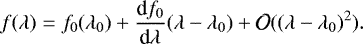
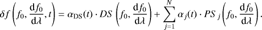
In the case of a small velocity shift, δv, with respect to the spectrum sampling, we can show via linearisation (first order of a Taylor series) that a shifted spectrum, f, can be expressed as the sum of a non-shifted spectrum, f0, and of the gradient of the flux multiplied by the difference in wavelength λ − λ0 for the same point in the shifted and non-shifted spectra (Bouchy et al. 2001):
 (1)
(1)
Using this formula and the fact that a Doppler shift can simply be expressed by δv∕c = δλ∕λ, we can show that:
 (2)
(2)
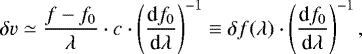
where δv is the Doppler shift and c the speed of light in vacuum. Thus, a velocity shift in that approximation regime is simply the linear coefficient between the flux variation (divided by the wavelength) and the flux gradient:
 (3)
(3)
Here DS stands for Doppler shell basis component and it represents, in the shell space, the behaviour of a pure Doppler shift. This denomination will become more clear in Sect. 3.3.
This finding leads to the observation that if we want to extract a velocity value, the gradient of the flux appears as a much wiser variable than the wavelength to characterise a spectrum, S. Moreover, keeping an information on the flux is primordial if we want to probe stellar activity signatures that are known to modify the line strength. Finally, to compute the velocity difference between a spectrum and a reference spectrum, we need to consider the observable δf. Therefore, as shown in Fig. 1, we decided to represent a spectrum in the space (d f0 ∕dλ, f) rather than the common one (λ, f). In addition, we added the extra dimension, δf (shown as a colour scale in Fig. 1) to be able to compute the RV difference between a given spectrum and a reference one. This transformation produces a compact representation of the spectrum where identical line profiles follow the same loop path. Hereafter, we refer to the (df0∕dλ, f, δf) space as the shell space and the projection of a spectrum onto this space S(d f0∕dλ, f, δf) as a raw shell, due to the resulting shape of a spectrum in this newly defined coordinate system. In the shell space, the core of the lines are located at a gradient of zero and a flux level smaller than 1, whereas all spectral points from the continuum are projected onto the same single point with flux unity and a null gradient. An example of the full spectrum of the G8 dwarf HD 10700 is displayed in Fig. 2 for a real Doppler shift.
To increase the S/N of a raw shell, we can bin the data in the shell space following a grid in normalised flux and flux gradient. Hereafter, we will call this binned raw shell simply shell. We note that the position of a bin in the (d f0 ∕dλ, f) space is the barycenter of all points in each cell, and its δf value is obtained by performing a weighted average on the δf of all the points within a bin, considering as the weight the inverse squared of the uncertainty in δf. For each bin, we calculate the corresponding S/N2 and only keep bins for which the S/N is larger than 1, to prevent being affected by noise occurring at the limb of a shell. We also discard the normalised flux level above 0.95 and below 0.05, since those regions do not contain significant Doppler information. In Fig. 3, we can see for HD 10700 the fraction of spectral points, as well as their mean wavelength, which fall into each bin of the raw shell defined by a 9 × 9 grid. We highlight that only 39.8% of the spectrum is used, since the remaining part is made of the stellar continuum which is discarded.
Using this shell representation, we can observe that the relevant parts of the spectrum that are sensitive to Doppler shift, which are the part with the highest absolute flux gradient value, represent a very small fraction of the total spectrum. Indeed, the bins with a value |df0∕dλ| > 4.4 only represent 39.8% ⋅ 18.1% = 7.2% of the total spectrum. Doing a similar analysis for the K1 dwarf HD 128621 leads to a similar value of: 60.4% ⋅ 15.3% = 9.2%. This observation explains why localised systematics can strongly affect the overall stellar RV even if the contamination appears in a small portion of the spectrum (Cretignier et al. 2021).
Finally, we observe that the positioning of spectral points in the shell space follow a colour dependence, which demonstrate that, opposite to a “white” CCF, the shell representation can be sensitive to chromatic effects. However, the small fraction of stellar lines in the red spectral range produces a reduced wavelength span compare to the full span of the spectrum, with average values ranging between 4200 and 5200 Å (see colourbar of Fig. 3). For this reason, shells are more dedicated to disentangle line depth and asymmetric line shape variations than chromatic ones.
The shell representation presented in this section allows us to solve most of the issues mentioned in Sect. 2 when analysing spectra or CCF time series. For an analysis of spectral variations using PCA, this new representation is more appropriate than the spectra themselves as it provides data with a much higher S/N. This new representation also contain more information than a CCF as: (i) red lines, that are broader than blues lines3 for a fixed velocity width and similar depth, will follow different loop paths; (ii) deep lines and shallow lines can be differentiated; and (iii) the velocity δv can simply be obtained by performing a linear least-square to estimate the linear coefficient between δf and the flux gradient. We note however two remaining issues. First, some degeneracies brought by line blending, which could be partially lift off if the second derivative of the flux was also included, however, this would lead to region of the (f,f′,f″) space with low S/N which is not desired (see already the low fraction of spectral point per bin in Fig. 3). Secondly, we point out the necessity of obtaining a reference spectrum, which is not straightforward. Such a spectrum can be obtained by stacking spectra in the stellar rest-frame after subtracting a first guess for the RVs. This method was in fact already implemented in YARARA and represents the main philosophy of the pipeline, where a master spectrum is constructed directly from the observations.
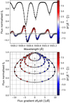 |
Fig. 1 Projection of a small part of a spectrum into the (df0∕dλ, f, δf) space that we call the shell space. Top: reference spectrum used to perform the change of variables (in black). The coloured dots correspond to the value of δf when comparing a Doppler shifted spectrum to the reference spectrum. Bottom: projection of the Doppler shifted spectrum onto the shell space. Each point in this new space corresponds to an original point of the reference spectrum and the colour coding corresponds, as above, to the value of δf when comparing a Doppler shifted spectrum to the reference spectrum. Positions of the lines’ cores were indexed to make the identification easier. The mean velocity difference between the shifted and reference spectra δv can be recovered as the slope between the flux gradient and δf. |
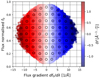 |
Fig. 2 Projection of the Doppler shifted spectrum onto the shell space for a real spectrum of HD 10700. The shell space has been dividedin a 9 × 9 grid (black lines) to increase the S/N of the raw shell after binning all the points within each cell. |
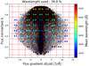 |
Fig. 3 Shell representation and statistics of a spectrum from HD 10700. Here, we highlight the fraction of spectral elements that fall within each bin, as well as their average wavelength (in colour scale). |
3.3 Decomposition of shells onto an orthogonal basis
In the previous section, we demonstrated the behaviour of a pure Doppler-shift on a shell. We recall that a shell is a spectrum projected onto the shell space, and then binned onto a 9 × 9 grid defined in the gradient flux and normalised flux dimensions. However, stellar activity, by inducing line-width broadening, line-depth, and bisector variations, will modify the shell in a different way than a pure Doppler shift would. Thus, if we could find an orthogonal 2D basis that describes a shell, we should be able to separate a pure Doppler-shift variation from a more complex perturbation induced by stellar activity or instrumental signals.
In order to separate Dopplerian components from other systematics, we have to define a basis of 2D functions that will be fitted on the shells, such basis will hereafter be called the “shells basis”. Those 2D functions have to be orthogonal with each other and should fit the variance of shells as much as possible. A PCA is therefore well suited to provide the optimal shell basis. However, the shell basis components derived by the PCA, PS, will not be orthogonal to the Doppler shell basis component. We thus used a Gram-Schmidt algorithm to guaranty orthogonality between the PS and DS shell basis components. With such a basis, a shell at time t can be written as:
 (4)
(4)
Looking at the equation above, it may seem that several options are on hand to correct for non-Dopplerians signatures, but the fact is that only one is well suited for the task. For instance, Eq. (4) cannot be used to correct the spectra in flux since no bijection exist from shells to spectra due to the mentioned degeneracy induced by blended lines. Another solution would consist of simply extracting the αDS (t) coefficient related to the Doppler shell (equivalent to δv in Eq. (3)), somewhat equivalent to a template matching method. However, this coefficient is generally almost identical to the CCF RV time series and therefore does not improve the RVs strongly. This can be understood, since no fundamental reason can justify why both stellar activity and instrumental systematics could not present a real Doppler-shifted component affecting as well αDS(t) (see Sect. 4.2.1). However, it is really unlikely for those contaminations to solely provide a Dopplerian component without presenting simultaneously non-Dopplerian effects (Huélamo et al. 2008; Meunier et al. 2010; Reiners et al. 2013; Marchwinski et al. 2015; Fischer et al. 2016; Davis et al. 2017; Barnes et al. 2017; Zechmeister et al. 2018; Dumusque 2018; Cretignier et al. 2020a; Lisogorskyi et al. 2021; Lienhard & Mortier 2021) that would be modelled by the PCA shell basis components. As a consequence, the best option remains to decorrelated in the time-domain αDS (t) with the other coefficients α(t), an option also chosen by the SCALPEL method (Collier Cameron et al. 2021).
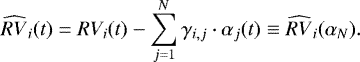
Instead of correcting αDS(t) or the CCF RVs, we chose to correct the LBL RVs by adding the αj (t) shell coefficients in the multi-linear model that will be fitted:
 (5)
(5)
A similar result would be obtain by decorrelating the CCF RVs, but the study of the γi,j can provide deeper information on the nature of the fitted components, in order to assess the origin of a component (from stellar activity or instrumental systematics). By averaging as in Dumusque (2018), the LBL RVs obtained in Cretignier et al. (2021) produce the average RVm(t) time series that will be used in this work.
Some concern may be raised about the number of PCA shell basis components that have to be fit. This is not a simple question to answer, as the number of relevant components change as a function of the S/N and with the total number of observations. Fitting too many components that are mainly noise-dominated would solely result in an undesirable noise increase in the fitted model or an overfitting. On the contrary, under-fitting would imperfectly correct for the contaminations. Therefore, a trade-off has to be found which can be accomplished by performing cross-validation (see Appendix A). In summary, our cross-validation algorithm measures the occurrence rate of PCA shell basis components by selecting random subsets of observations. For the present paper, we performed 300 independent sub-selections of the shells time series by randomly removing 20% of the observations. In the end, we only considered the PCA shell basis components having an occurrence rate higher than 95% as significant.
4 Results
In this section, we demonstrate the applications of the shell decomposition presented in Sect. 3.3 on two HARPS datasets that present high S/N and an exceptional sampling. We first analyse the data of HD10700 that present no sign of stellar activity and no significant planetary signals (see however the very small amplitude candidates published by Feng et al. 2017). This dataset will be used to prove, similarly to what was done for YARARA in Cretignier et al. (2021), that our shell approach does not absorb any injected planetary signals with amplitudes smaller than 3 m s−1. We then analyse the data of HD 128621 to show that our shell approach can significantly correct for stellar activity. Test of planetary signal injection into the HD 128621 dataset also show that in that case, the planetary signal is fully recovered despite strong stellar activity modulations in RV. Finally, we estimate the S/N that is required to mitigate the stellar activity signal in HD 128621 using our shell approach.
4.1 Planetary injections on HD 10700
HD 10700 (τ Ceti) is a bright G8V star of magnitude mv = 3.5 with a peculiarly low activity level. Opposite to HD 128621 who shows clear evidence of stellar activity manifestation, HD10700 has never exhibit any strong evidence of activity over the two decade of HARPS observation and is likely the quietest star in the solar vicinity. Such unusual behaviour could be explained either by a perturbation of the stellar magnetic cycle similar to the solar Maunder minimum or by the star being seen pole-on. As a consequence, HD 10700 has been intensively observed as a standard calibration star during the full lifetime of HARPS in order to track instrumental systematics and search for very low-mass planets.
Here, we analyse ten years of the HD 10700 HARPS dataset gathered before the fibre upgrade in June 2015. In Cretignier et al. (2021), we demonstrated that by post-processing the spectra with YARARA, which removes most of the known instrumental systematics, a RV precision of 1 m s−1 can be reached overthose ten years. To perform a planetary signal recovery test, we used the same dataset as in that paper, since the injected planets – with 3 and 2m s−1 signals at 122.4 and 37.9 days, respectively – were dominating the RV variation. As in Cretignier et al. (2021), the planets were injected at the spectrum level by first correcting the systematics, Doppler-shifting the cleaned spectra with the Keplerian solutions, and finally re-introducing the removed systematics before re-running YARARA.
On the left of Fig. 4, we plot the shell basis components (the first PCA basis components in addition to the DS basis component) that we obtained after applying the shell decomposition presented in Sect. 3.3. Once the optimal basis is found, each shell that is obtained after projecting each stellar spectrum onto the shell space and binning it is expressed as a linear combination of the differentj componentsof the basis (see Eq. (4)) and the related coefficient αj (t) are saved. For each basis component, j, we therefore obtained a time series αj(t) and we show the plot of its corresponding Generalised Lomb–Scargle (GLS) periodogram in the middle of Fig. 4. All the falsealarm probability (FAP) used in this paper for the different periodograms were obtained by bootstrap of 10 000 random permutations. On the right of Fig. 4, we show the results of our cross-validation analysis, described in Appendix A, which estimates whether the shell basis components are significant or not. Thisanalysis shows that the first four shell basis components are found significant (the matrix of the cross-validation algorithm can be found in Fig. B.2). Finally, in the last subplot of Fig. 4, the periodogram at the very bottom of the figure corresponds to the GLS periodogram of the residuals,  (see Eq. (5)), after all the significant PCA shell basis components have been fitted.
By looking at the shell basis component in Fig. 4, we clearly see that all shells present a clear and smooth structure. For the PCA algorithm, each point of the shell is considered independent, and thus the algorithm has no constraints that would produce a smooth shell except if the physical process perturbing the line profile is itself a smooth perturbation. This is, of course, something that is expected from both stellar activity and instrumental systematics.
We clearly see in Fig. 4 that the 37.9 and 122.4-day planetary signals are completely captured by the DS shell basis component. Other peaks surrounding the periods of the injected signals are the one-year aliases (see e.g. Fischer et al. 2016; VanderPlas 2018) due to the window function produced by the gap between the observational seasons. We also observe some power around 122 days for the first and fourth components. This period is not the dominant signal of respective periodograms and does not correspond to the 122.4-day injected planet. This power seems to be produced by the window function of a one-year systematic corrected. Indeed, it can be shown that by generating a perfect one-year signal with the time sampling of the observations, the GLS periodogram clearly presents significant power at one-year, but it also does so at its first two harmonics as well.
The time series of the coefficient αDS(t) fitted for this shell component correlates perfectly with the classical CCF RVs ( ). Despite those planetary signals being strong in the DS shell basis component, we investigated by how much the planetary signals were affected by the linear decorrelation with the αj shell basis coefficients. We thus fitted a non-eccentric two-Keplerian solution on the residuals
  by fixing the periods of the injected planets, and we recovered amplitudes of 2.83 m s−1 and 2.00 m s−1 for the 3 and 2 m s−1 injected planetary signals, respectively. We note that the period of the planet after YARARA post-processing was in fact already recovered at 2.85 m s−1 (Cretignier et al. 2021). This was perfectly explicable by the known presence of lower amplitudes signals around this star (Feng et al. 2017). By fitting all signals more significant than a FAP of 0.1%, the planetary amplitudes change to 2.95 and 2.03 m s−1, respectively, indicating some cross-talk between the injected planets and pre-existing lower amplitude signals.
As mentioned in Sect. 3.3, only the PCA shell basis components are orthogonal to the DS shell basis component, but not the αj coefficients with respectto αDS(t). As a consequence, all planetary signals would be slightly projected on the basis of the αj (t) coefficients, and the best way to account for this is to include the planetary signals in the multi-linear regression and perform a Monte Carlo Markov chain to measure the degeneracy. We note however that such projection is reduced when the number of observations increases and nearly vanishes for HD 10700 due to the large number of observations.
Assessing the question of the minimal number of observations required is difficult to answer. First, because the observationsshould probe different ‘levels of contamination’ in order to allow the PCA to detect the flux variations and, secondly, since with lower number of observations, the degeneracies of the full Keplerian model increases, which itself depends on: the model complexity, the period of the planetary signals, and power spectrum of the αj (t) basis. Despite the difficulty in estimating a number on the basis of too many unknown parameters, there is a simple way to estimate the degeneracy.
To measure such collinearity effects under the assumption of a unique planetary signal in circular orbit, which allow for a fast computational time, we can simply simulate a sinusoidal variation with a given period and phase and with an arbitrary amplitude, K, evaluated on the time sampling of the observations; we then project this signal on the αj basis with a linear least-square and measure the residual amplitude, Kres. We note that because the contamination model consist of a simple multi-linear regression (see Eq. (5)), the amplitude of the simulated planets does not influence the relative absorption of the signal. We simulated 18 different phases and 15 000 different periods equidistant in frequency from three days up to the length of the observational baseline. The relative absorption and standard deviation of a sinusoidal signal, after averaging the different phases, are displayed in Fig. 5 for HD 10700. We observe that for the data of this star, none of the injected signals are absorbed by more than 13% in average, which is in line with the small number of components (only four) with respect to the 406 data points fitted. As a general rule, an increase towards longest periods is observed, simply due to the fact that long-terms signal are more degenerate than shorter ones for dense observational sampling due to the finite length of the data set.
For the 37-day injected planetary signal, the absorption is negligible (only 2% in average) whereas that for the 122-day signal, a relative amplitude difference of 7 ± 4% is observed. Such an analysis is only valid in the case of multi-planetary non-eccentric signals, as long as there is no cross-talk between the planetary signals, which can happen in the case of poor sampling with regard to the signals. Even if the best strategy remains to include the αj(t) basis coefficients inside the fitted Keplerian model, an analysis such as the one presented above, can be used to estimate with a data-driven approach by how much planetary signals can be absorbed. This planetary signal injection-recovery test confirms that the shell decomposition is perfectly able to disentangle Doppler shift from others contamination (as instrumental ones here) and that the planetary signals are not significantly absorbed.
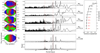 |
Fig. 4 Shell decomposition of HD 10700 spectra. Left: representation of the different shells basis components and the time series of the coefficients αj(t) in fronteach of those shell basis components when modelling the RVs of HD 10700 (see Eq. (4)). All the components are orthogonal to the Doppler shell basis component (DS) displayed at the bottom (similar to Fig. 2) thanks to a Gram–Schimdt algorithm. The pixel grid in the shell space on which the PCA was trained (dots) is shown, as well as a smooth function interpolated on the full shell space using a cubic interpolation algorithm. Middle: generalised Lomb–Scargle periodogram of the αj (t) shell component coefficients. The 0.1% false alarm probability (FAP) level for each periodogram is indicated by an horizontal dotted-dashed line. From top to bottom, we can see the five first principal shell basis components and the DS. The Pearsoncorrelation coefficient between the αj(t) and the CCF RV time series is indicated on the right side of each subplot. The lowest periodogram represents the RV time series linearly decorrelated from the αj coefficients (similar to Eq. (5)). The power at the planetary injected periods (vertical red lines) is never the dominant power for any shell. This is particularly true for the 37-day signal less significant than the 0.1% FAP level. Some power is observed around 122 days for PS1 and PS4 due to an alias of a one-year systematics (see main text). Right: explained variance curve of the PCA components. Our cross-validation algorithm (see Appendix A) provides four significant components (> 95%). The components compatible with a single outlier explanation (<80%) are shown in red. |
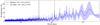 |
Fig. 5 Measurement of the collinearity between planets in circular orbits and the αj (t) basis for HD 10700. The simulations are made of 18 different phases and 15 000 different periods. The envelope describes the 1-sigma dispersion obtained from the different phases for the same period. The injected planets are marked by vertical lines. A typical decrease of 2 ± 1 and 7 ± 4% can be expected for the 37-day and 122-day planets, respectively. Those results are coherent with the ~ 2 m s−1 and ~ 2.85 m s−1 planetary signals recovered, while the original signals injected for those planets was 2 and 3 m s−1, respectively. |
4.2 Correction of stellar activity on HD 128621
We then tested our shell framework on HD 128621 (α Cen B, K1V, magnitude mv = −1.3), a star that exhibits a similar activity to the Sun and is thus more active than HD 10700. From 2008 to 2012, the star was on the increasing part of its magnetic cycle, such that the 2010, 2011, and 2012 seasons clearly exhibit strong signatures of stellar activity at the 36-day rotational period (e.g. Dumusque et al. 2012). We analysed the 2008 to 2012 HARPS dataset of HD 128621 post-processed by YARARA (Cretignier et al. 2021) due to its exquisite quality and the presence of clear stellar activity features.
We first investigated the impact of the YARARA post-processing on the LBL RVs. In Cretignier et al. (2020a), for the 2010 dataset, we demonstrated that most of the lines presenting strong RV signals correlated with activity were simply blended lines changing either in depth or width. This effect produced an unexpected physical result from the CBI point of view, namely, the production of lines anti-correlated with stellar activity. Since YARARA decorrelates the flux time series at each wavelength by fitting the contrast and the full width half maximum (FWHM) of the CCF, YARARA should correct for this effect, which is indeed observed in Fig. 6. In that figure, we display the polar periodogram (Cretignier et al. 2021) at 36 days for the LBL RVs of the 2010 dataset. We also indicate several activity proxies used commonly in the literature as well as the new αj shell basis coefficients. We clearly see that lines anti-correlated with the S-index at ϕ = 180°, as by definition ϕ = 0° corresponds to the phase of the S-index time series, completely disappear after YARARA post-processing. We are thus left with lines that are all correlated to some level to the S-index, which is coherent with the CBI theory.
In Figs. 6 and 7, we can observe that for each active season (2010 to 2012) the distribution of spectral lines in the polar periodogram is clearly anisotropic in the angular coordinate, which indicates an excess of power at the rotational period in a GLS periodogram. We note that the highest peak in the periodogram was found around 40 days rather than 36 days in 2012. Also, different phase lags can be observed between the average phase of all the spectral lines and the phase of the S-index. When it is in phase in 2010, the phase lag in 2011 and 2012 is ~ 90° and ~ 45°, respectively. We note that the precise phase lag measurement depends on the choice of the period due to the covariance between both parameters. Such phase lags explains why linearly decorrelating the RV time series with the S-index time series does not mitigate stellar activity and why kernel regression (e.g. Lanza et al. 2018) or Gaussian Process (GP) regression (e.g. Rajpaul et al. 2015) allow for an improved mitigation stellar activity signals.
4.2.1 Shells decomposition of HD 128621
We performed the shell decomposition described in Sect. 3.3 on the HD 128621 YARARA post-processed data set. We display in Fig. 8 the shells fitted as well as the corresponding GLS periodogram associated with the αj coefficients. As for HD 10700, we decided to inject a planetary signal at 54 days and with a semi-amplitude of 1.5 m s−1 (7.5 M⊕ for a 0.80 M⊙) in order to assess the ability of shells to disentangle stellar activity from planetary signals. Only four components were found to be significant and we observe once again the remarkable smoothness of those shells, (which is not a condition required by the PCA), indicating a smooth perturbation of the line profile induced by stellar or instrumental systematics. We clearly observe the rotational period of the star close to 36 days in all the components. However, α3 also present excess power at one year related to instrumental systematics, which is due to the fact that the PCA is not able to separate the different contaminations. In fact, it is expected that stellar activity and instrumental systematics will be mixed in the PCA shell basis components, even if most of the time one effect will dominate over the other. We note that the fourth basis component coefficient time series, α5, is found to be significant by the cross-validation algorithm and presents power excess around the rotational period, whereas α4 is not found significant and is therefore discarded. For the remainder of this paper, we use the name convention from Eq. (5) (indices based on the RV fit) rather than Eq. (4) (indices based on PCA) to avoid gaps in components indices; therefore, we denote the previously mentioned α5 as α4.
We modelled the CCF RVs – or, equivalently, the αDS(t) DS shell basis component coefficient – using our multi-linear regression composed of the αj shell basis coefficient time series (see Eq. (5)). The highest peak recovered in the RV residuals is the injected planet at 54 days, with the other peaks at 47 and 63 days standing as the one-year aliases of the injected planetary signal. This demonstrates the ability of such method to disentangle pure Doppler shift signals from stellar and instrumental contaminations. In addition, the K semi-amplitude of the planet fitted on the corrected RVs is found to be 1.37 m s−1, which is only 8% smaller than the injected value. By performing the same simple sinusoidal signal projection as for HD 10700 (see Sect. 4.1), a value of 3 ± 2% of absorption is found (see Fig. 9), which is compatible at 2.5σ with the measured absorption of 8%. The slightly higher observed absorption can be explained by the interaction with pre-existing signals in the original data set. When fitting for the 54-day Keplerian signal on the planetary-free data set (scanning slightly around the period), 10 cm s−1 K semi-amplitude signals are typically measured, which amount to about 7% of the injected semi-amplitude 1.5 m s−1. Therefore, an uncertainty of 7% on the recovered amplitude is expected simply from the pre-existing structures inside the initial data. The maximum absorption is about 25 ± 5% at 39 days, which matches the suppression of the 39-day signal in the GLS periodogram. Therefore, even a real planet at 39 days would not be absorbed at a higher level than 25%, on average. This can be explained by the fact that our shell framework is optimised to model the change of phase and period of the stellar activity signal seen on HD 128621, and thus cannot properly model a pure sinusoidal variation induced by a circular planet. This is also an advantage brought on by multi-linear models that are more rigid than kernel or GP regressions and that are therefore less likely to absorb planetary signals.
By looking at Fig. 8, we can clearly see that the DS shell basis component also contains an activity component, as shown by the excess of power around 36 days. This behaviour does not, in fact, contradict the stellar activity. Indeed, from the CBI point of view, even if a stellar line is affected differently depending on some underlying properties, such as its formation depth in the stellar atmosphere, the element, or its wavelength, we can naturally expect that all the lines are affected by a common average effect; therefore, a real Doppler shift. This has already been seen in Cretignier et al. (2020a), when the authors derived a relation between inhibition of the convective blueshift and depth of spectral lines (see Fig. 8 of that paper). As soon as blended lines were removed, 90% of the lines presented a RV signal correlated with stellar activity, and the minimal amplitude was 3.3 m s−1.
The presence of a real Doppler shift component from stellar activity is not a substantial issue (as already explained in Sect. 3.3). Indeed, even if the CBI can present a real Doppler shift component, it will also induce line distortion, which wouldbe modelled by the different shell basis components. Thus, CBI is not solely a pure Doppler shift. By investigating the PCA shell basis components, the first one is the most related to the inhibition of the convective blueshift, since the α1 coefficient time series is strongly correlated with the CCF RVs ( , see correlation in Fig. 8).
For the forthcoming analyses, we redid the shell decomposition without the injected planet to avoid the complexity brought by this extra signal. We note that we obtained the same shell basis, as the planetary signal is completely captured by the Doppler shell basis component.
We performed a comparison between the shell basis component coefficients and classical activity proxies, namely, the CCF moments and CaII H&K. The correlation matrix is displayed in Fig. 10. The CCF moments are computed without the YARARA correction for stellar activity, since after this step, the CCF contrast and FWHM no longer present any stellar activity signatures. However, since the CCF moments and CaII H&K are affected by an extended magnetic trend, we systematically fit a second order polynomial function on all the time series to produce an homogeneous analysis that is focussed on the rotational period. As we can see, when the shell decomposition is performed without the injected planet, the correlation between α1 and the RV time series is even stronger ( while it was 0.45 in Fig. 8). The second shell basis component also captures stellar activity as it is strongly correlated with the VSPAN of the CCF (
 ) and shows a phase lag of 90° with the RVs, which explains the low correlation among them (
 ). Overall, we observe that some correlations exist between the CCFs moments and the shell basis component coefficients, αj, which clearly indicates an indirect connection between the CCF and shell spaces.
We note that no shell basis component alone is able to correct efficiently for the stellar activity in RV. It is only when combining all of them together that the stellar activity mitigation is optimal. This is visible in Fig. 6 and 7, where none of the αj coefficients are in phase with the RVs simultaneously for 2010, 2011, and 2012; whereas it is only the complete multi-linear model (pink square) that gives (roughly) the correct phase for each observational season. This indicates that several different perturbations of the line profile are in play, likely induced by different type of active regions (spots versus faculae) or active regions with different intrinsic properties evolving over time (temperature, size, location, or magnetic field strength).
In Fig. 11, we display the periodogram of the residuals RVs as a function of the number of αj coefficients fitted. It can be seen that the rotational period is strongly mitigated after the inclusion of three shell basis coefficients into the multi-linear model. The second coefficient, α2, is barely effective in improving the RVs due to the previously mentioned phase lag of 90° with respect to the RVs. To demonstrate that shell basis coefficients and CCFs moments are different, despite their correlations, we also display in the bottom panel of the same figure the residuals obtained by fitting the contrast, FWHM, and VSPAN, as well as CaII H&K using a similar multi-linear model. The obtained result clearly demonstrates that the averaging nature of the CCF produces moments that are not as good as the shell basis coefficient in mitigating stellar activity.
Interestingly enough, we observe that both model produce similar rms for the RV residuals, but completely different periodogram. Using our shell framework, the RV rms over the five years of HD 128621 observations is improved from 2.44 m s−1 down to 1.73 m s−1 (against 1.72 m s−1 using CaII H&K and CCF moments). This example demonstrates that RV rms is not an optimal metric in the context of stellar activity and a periodogram remains a more relevant statistical tool. For that reason, we also computed a second score metric defined as the integrated power between 32 and 45 days, which is the period range capturing the 36- and 40-day signals (rotational period measured in 2010 and 2012) and their respective one-year aliases. Despite the similar rms, the model obtained from the shells clearly demonstrate an higher ability to absorb power at the activity-related signals with a score reduced by a factor 2.51 against only 1.29 for CCF moments. We also note that CCF moments obtained on spectra corrected of YARARA do not present any more activity signatures and cannot be used to correct the RVs.
Once we have demonstrated what shells can do, we can try to better understand what they represent. Getting a feeling about the line profile distortion is not always evident from the spectrum-folded representation of the shells. In order to better perceive the meaning of the PCA shell basis components, we project them back onto the classical line profile space. To do so, we performed a cubic interpolation of the shell basis components on the restricted (f′, f) domain of a spectral lines with different depths. We remind that because of the degeneracies brought by blended lines, no bijection exist between shells and line profile and therefore such transformation should not be fully interpreted as the real line profile modification but, rather, it ought to carry an equivalent interpretation of the shells into the classical line profile space.
We generated three Gaussian lines at 5250 Å with a FWHM of 6 km s−14 and three different line depths and extracted the δf variation related to the four first PCA shell basis components displayed on the left of Fig. 8. We show the result of the inverse projection in Fig. 12. We observed that the PS1 component is roughly equivalent to a bisector change for shallow lines, a core depth variation for medium lines, and a core broadening for deep lines. Interestingly enough, all those modifications are line profile variations expected from a stellar activity point of view and are here all inter-connected within the same shell basis component and related coefficient α1 (t). Carrying out a similar exercise based on PS2, we find that this coefficient is equivalent to a bisector change, independently of the line depth. This is coherent with the strong correlation observed between α2 (t) and CCF VSPAN (see Fig. 10). The third component PS3 seems equivalent to a wings broadening, independent here again of the line depth. Finally, the last component PS4 seems once again to be related to a change in the bisector.
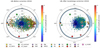 |
Fig. 6 Polar periodogram for the 2010 HD 128621 dataset obtained for a fixed period of 36 days, known to be the stellar rotation period of HD 128621. Each dot represents a spectral line. Peculiar activity proxies and αj (t) coefficient time series are shown as markers of different types (see legend). The radial coordinate is the weighted |

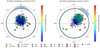 |
Fig. 7 Polar periodogram for the 2011 and 2012 HD 128621 datasets after YARARA correction. For 2012, the highest peaks in the periodogram correspond to a period of 40 days, so we display the polar periodogram at 40 days rather than36 days. A clear time-lag between the RV variation of each line and the CaII H&K (purple cross) of ϕ ~ 90° (9 days) and ϕ ~ 45° (5 days) is visible in 2011 and 2012, respectively. The RVs are however in phase with the multi-linear model of αj (pink square) as well as with the CCF FWHM (orange star). |
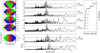 |
Fig. 8 Shell decomposition of HD 128621 spectra. The first shell is the one presenting the highest correlation with CCF RVs. The second shell is similar to a change of the line bisector and the time series of the related coefficient strongly correlated with the VSPAN of the CCF. Third shell, present mostly power at one-year and a half-year and is more related to instrumental systematics. The fourth component (fifth one according to the explained variance) seems once again to be related to stellar activity. The next components all possess a score lower than 80% and are therefore considered as less significant. After the decorrelation by the shell coefficients αj (t), the planetary injected period at 54 days (vertical red line) becomes the dominant signal, with the other peaks at 47 and 63 days being the one-year aliases. |
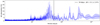 |
Fig. 9 Measurement of the collinearity between planets in circular orbits and the αj (t) basis for HD128621. A maximum of absorption of 25 ± 5% is observed for the rotational period of the star at 39 days. It demonstrates than even if the rotational signal is strongly mitigated, a real circular planetary signal at 39-days would not have been more absorbed than this. For the injected planetary signal at 54 days, the absorption is 3 ± 2%. Absorption at one-year and a half-year are also noticeable. |
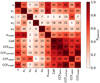 |
Fig. 10 Correlation matrix of the CCF RVs time series, v(t), the shell basis coefficients, αj(t), and the full model fitted with other common activity proxies. The different shells basis coefficients show weak correlations with the CCF moments highlighting an indirect connection between shells and CCFs. |
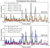 |
Fig. 11 Periodograms of the residuals RVs parametrised by the model complexity (name convention as in Eq. (5)). All the periodograms are normalised according to their respective 1% FAP level (horizontal dotted-dashed line). The RV rms of the residuals for each model is indicated in the legend as well as the integrated power between 32 and 45 days. Top: results obtained by increasingly adding shell basis coefficients into the multi-linear model of Eq. (5). Once three shell basis coefficients are fitted, the rotational period is no more significant (green and red). Bottom: comparison between the residuals obtained after fitting for four shell basis coefficients (red) or the three classical CCF moments (FWHM, VSPAN and contrast) plus the CaII H&K. Both CCF moments before (CCFY 0, blue) and after YARARA processing (CCFY 1, green) were used. |
4.2.2 Stellar activity mitigation with respect to S/N
In opposition to the CCFs that can be seen as the most optimal S/N projection of the spectrum, shells are at a lower S/N due to the less compact nature of the projection. For that reason, a reasonable question to address is the required S/N of the observationsneeded to correct for stellar activity using our shell framework. We note that throughout the paper, we use the S/Ncont notation to refer to the S/N of spectra in the continuum, to avoid confusion with the S/N of shells.
To test the S/Ncont required to correct for the activity signal seen on HD 128621, we injected different level of photon-noise at the spectral level. In total, we performed 26 different realisations of S/Ncont ranging from 50 to 650 by step of 25. More details about the precise process of noise injection can be found in Appendix C. Despite the exquisite quality of the HD 128621 observations, it should be noted that the S/Ncont of the observations are flat-field limited and therefore they never exceed (on average) the full spectrum S∕Ncont ~ 650 on HARPS (e.g. Cretignier et al. 2020b)
We performed the same shell decomposition as presented in the previous section, except that the cross-validation algorithm was not applied on the PCA shell basis components, as it would select fewer components at low S/Ncont (see below),which is not the purpose of the present evaluation. For the same reason, the S∕N > 1 criterion for each point in the shell was not applied, which implies that the same shell space was used for all the simulations. We chose to fit the five components in a constant way in order to get a similar model complexity for all the simulations, while recalling that four were found to be significant (as shown in Sect. 4.2) at the nominal S/Ncont values of the observations. The fifth component, which is therefore noise-dominated, will allow us to control the noise behaviour. The projection of the shell basis coefficients αj was performed on the raw RV time series without extra-noise injected. In that way, the simulations solely measure the degradation of the shells with respect to noise.
In the top left panel of Fig. 13, we represent the correlations between the shell basis coefficients without extra-noise injected, αj,obs, and the shell basis coefficients, αj, obtained after noise injection. In the top middle panel, we show the RV rms of the shell basis coefficients αj, obs projected onto the time-domain using the γi,j averaged over all the lines, < γj > (see Eq. (5)). In the top right panel, we display the RV rms of the modelled activity, as well as the RV rms of the residuals after this model has been fitted to the RVs for different S∕Ncont. Finally, in the bottom panel, we show the periodogram of the RV rms of the residuals after fitting for the shell basis components obtained for four typical S/Ncont simulations, namely, S∕Ncont = 50, 150, 250, and 350. In the following, we discuss the result for those four typical S∕Ncont.
At S∕Ncont = 50, our lowest S/Ncont injection test, the shell basis components are mostly noise-dominated and no significant improvement is observed in the RVs after correcting them using our shell framework. At S∕Ncont = 150, the two first shells basis coefficients, α1 and α2, that are related to stellar activity are clearly detected ( ) but we only performed a partial correction since α3 is not yet recovered. At S∕Ncont = 250, the power of the periodogram peaks related to stellar activity is now smaller than the 1% false alarm probability level (see bottom panel of Fig. 13). It is only after S∕Ncont = 350 that the third shell basis coefficient α3 is recovered. From this S/Ncont value, the RV fitted model stop to significantly mitigate stellar activity. From S/Ncont = 350 to S/Ncont = 650 the only notable observation is the recovery of α4, which becomes fully detected at S/Ncont = 550, but we already demonstrated in the previous section that most of the stellar activity correction was performed by the fit of α1, α2, and α3, which is also highlighted in the top middle panel of Fig. 13; here, we see that the α4 shell basis coefficient projected onto the RVs is only responsible for a RV rms smaller than 50 cm s−1. We therefore conclude that the minimal S∕Ncont required to optimally correct for the stellar activity signal in HD 128621 is 250.
The present limitation in S∕Ncont is mainly induced by noise in the shells that are fitted by our model. We perform a second iteration of the previous simulations, this time including the S∕N > 1 criterion on the shell elements and the cross validation algorithm. We display, for both cases in Fig. 14, with or without the S∕N > 1 criterion and cross-validation, the integrated power between 32 and 45 days of the residuals RVs, which contain most of the stellar activity signal. The number of significant components found by the cross-validation algorithm is 0, 2, 3, and 4 for S∕Ncont = 50, 150, 250, and 350, respectively. This validates the ability of our cross-validation algorithm to reject noisy components. Moreover, by imposing S∕N > 1 and the cross validation, we can strongly mitigate stellar activity starting at a S∕Ncont = 200 instead of S∕Ncont = 250 with the five-component model.
It should be noted that those noise injection tests do not take into consideration the degradation of the YARARA performance with the S/Ncont, nor the degradation of the RVs themselves – thus, these are optimistic results. Furthermore, those threshold S/Ncont limits are solely valid for the present α Cen B activity signal. Based on real data, these tests however do demonstrate – similarly to what was done by Davis et al. (2017) on simulated data – that a very high S/Ncont is required to correct for stellar activity signals in RV measurements. This should certainly be considered for current and further RV surveys aiming at confirming or finding the smallest amplitude planetary signals.
Considering that activity on HD 128621 induces a RV rms of ~ 1.72 m s−1 (quadratic difference between 2.44 m s−1, the raw RV rms before the shell correction, and 1.73 m s−1 after correction), and that this signal is scaling linearly with the δf variation of the spectra (see Eq. (2)), the minimum S∕Ncont value required to correct for a specific activity jitter can be given by:
 (6)
(6)
Reaching such a high S∕Ncont is not achievable for any star and telescope that put strong constraints on the observational strategies needed to correct for stellar activity with the present method. We note, however, that the shell method presented here is a data-driven approach that needs to detect the signal at the spectral level (or shell level in our case) and thus it is unlikely that other data-driven approaches could do better. On a positive note, HD 128621 is not a peculiar active star considering its mean log ( ) = −4.94 value and, therefore, the value of S∕Ncont = 250 can be considered as representative for this spectral type.
Once the rotational peaks disappear, new periods become significant around 19 days. It is expected that stellar activity produces not only power excess at the rotational period but also at the rotational harmonics (Boisse et al. 2011; Borgniet et al. 2015; Collier Cameron et al. 2019). Nevertheless, this 19-day signal could also satisfy the period of a potential transiting planet observed with Hubble (Demory et al. 2015) to confirm the debated existence of α Cen B b (Dumusque 2012; Hatzes 2013; Rajpaul et al. 2016). However, when extracting the Keplerian solution, the transiting phase of the signal did not match the potential transit ephemeris and we therefore believe that this signal is the first harmonic of the stellar rotation. The analysis of solar data (Dumusque et al. 2021) by our shell method will be presented in a forthcoming paper. We can, however, already mention that a similar result was found – namely, the finding that the rotational period can be fully corrected but its first harmonic tends to be more resistant to our corrections. One solution could be to include the time derivative of the proxies in the modelling (Aigrain et al. 2012). We note that, intuitively, we could expect that spot and faculae, which are known to contribute in various ways to the RV budget (Meunier et al. 2015), could produce power at different harmonics due to the respectively even and odd nature of their RV signal according to the stellar meridian (Dumusque et al. 2014). The persistence of a RV signal at the first harmonic of the rotational period is perhaps a sign that our method is less sensitive to specific active regions. It is however unclear for the moment if this is due to the fact that shells cannot detect their signature or because the multi-linear model is overly simplistic.
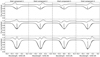 |
Fig. 12 Inverse projection of the four significant PCA shell basis components, shown on the left of Fig. 8, used to correct the RV time series of α Cen B. The inverse projection was realised for Gaussian line profiles at 5250 Å with a FWHM equivalent to 6 km s−1 and threedifferent line depths (0.2, 0.45, and 0.7, from top to bottom). The delta flux variations, δf, evaluated along the line profile chord (see Fig. 1) are indicated after magnification above the Gaussian line profile and compared with δf = 0 (horizontal dotted line). The bisector of each line profile is also indicated after magnification and compared to the initial Gaussian profile (vertical dotted lines). |
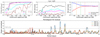 |
Fig. 13 Noise injection tests performed on HD 128621 to evaluate the performance of our shell framework in mitigating stellar activity depending on the continuum signal-to-noise ratio, S∕Ncont. The cross-validation algorithm to select only shell basis components with significant variance was disabled and five componentswere used for the fitted model. Top left: correlation between the noise-affected shell basis coefficients αj and their respective coefficients without extra-noise injected αj,obs. A shell basis component can be considered as recovered once its related coefficient αj exceeds a correlation value with αj,obs higher than |

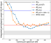 |
Fig. 14 Noise injection tests performed on HD 128621 to evaluate the performance of our shell framework in mitigating stellar activity. In this figure, we show the dependence between the integrated power of signals between 32 and 45 days, which contain mostly stellar activity signal, and the S∕Ncont. Previous values mentioned in Fig. 11 and obtained at observed S∕Ncont values (~650) are reported (solid horizontal lines). Activating the cross-validation algorithm to select only shell basis component with significant signal and imposing the S∕N > 1 criterion to reject noisy shell elements allow to mitigate significantly stellar activity starting at a S∕Ncont = 200 (orange curve) instead of S∕Ncont = 250 (blue curve). One thousand random realisations of white noise with the time samplingof the data were produced to get a reference power value, given at ± 1σ (gray area). |
5 Discussion and conclusion
In this paper, we present a novel approach to correcting for non-Dopplerian signatures in stellar spectra, such as those introduced by stellar activity and instrumental signals. The method consists of projecting stellar spectra into a dimensional space where the spectral information is averaged-out, but not as much as in the CCF space. Contrary to the CCF, a spectrum projected into this new space contains information about the line depth and chromaticity, which are known to be influenced by stellar signals.
Mathematically, the projection consists in looking a spectrum in the space (f, f′, δf), namely, the flux derivative, normalised flux, and flux difference between the spectrum and a master spectrum divided by wavelength. As δf∕f′ = v∕c, where v is the Doppler shift and c the speed of light, such a space is particular suitable for the study Dopplerian and non-Dopplerian components (see Sect. 3.2). A spectrum projected into this space, which we call a raw shell, is then binned in the (f, f′) space to increase the S/N and produce what we call a shell. The time series of shells can then be fitted using a PCA algorithm to produce an orthogonal shell basis made of the principal components (Sect. 3.3). We then add an extra Doppler shell basis component and perform a Gram-Schmidt algorithm to have all shell basis component orthogonal to each other. The time series of the fitted shell basis coefficients, excluding the one from the Doppler shell basis, are ultimately used to linearly model non-Dopplerian RV variations.
We demonstrate that the framework adopted here does not absorb any real planetary signal, but it can effectively mitigate instrumental systematics (Sect. 4.1) and the stellar activity signal seen at the stellar rotational period (Sect. 4.2). Planetary signal injection tests performed on HD 10700 show that our shell framework allows us to correct for instrumental systematics that is found at a period of a year and half a year, while absorbing the planetary signal by not more than 13% in the worst case. In the case of HD 128621, we show that a planetary signal is not altered when applying our shell framework, and furthermore, the stellar activity signal estimated to induce a RV jitter of 1.72 m s−1 (quadratic difference between 2.44 m s−1, the raw RV rms before the shell correction, and 1.73 m s−1 after correction) is strongly mitigated to a non-significant level. We also noted that the first harmonic of the stellar activity signal at 19 days was difficult to correct, which may indicate that more advanced correction models should be deployed to account for the rotational harmonics.
The transformation from a spectrum into a shell is not bijective and, thus, it is not possible to project the shell basis back into the spectrum space. We thus have to correct for systematics in the time-domain – and not in the flux-domain. This implies that collinearity between our shell basis coefficients and planetary signals can always occur, and therefore, we have to model RV systematics and planetary signals simultaneously to prevent such eventuality, as done in SCALPEL (Collier Cameron et al. 2021). This will be formally implemented in a subsequent paper, where we will further improve the RVs to correct for the last remaining instrumental systematics.
Working in the shell space where the representation of a spectrum is at a lower S/N than the CCF has a drawback, nonetheless. Indeed, simulations performed in Sect. 4.2.2 demonstrate that our shell framework is efficient at mitigating the stellar activity at the rotational period of HD 128621 only for spectra with S∕Ncont > 250. This conclusion strongly motivates us to pursue previous intensive observational strategies of multi-observations per nights (Dumusque et al. 2011a), which is a natural strategy used to boost the S/N and mitigate shortest stellar signals such as the ones induced by oscillation modes and granulation. The spectra could be stacked on several days if the rotational period of the star is long enough, but in any case, this requires stars with intensive observational strategy and observations almost every night. An intense effort already known to be paramount to detect Earth-like planets (Thompson et al. 2016; Hall et al. 2018; Gupta et al. 2021).
Because the noise injection tests only measure the efficiency of the PCA algorithm to recover significant shell basis components despite noise, the demonstrated S∕Ncont = 250 limit could theoretically be relaxed if the data-driven method was replaced or combined with a physically motivated approach, making the PCA algorithm unnecessary. Therefore we want to use future studies to explore whether the same shell basis could be used for stars of similar spectral type or if those shell bases are somehow related to the atomic physics of spectral lines.
Possible ways to improve the current work would be to fit the new proxies found here, namely, the time series of the shell basis coefficient, with a more complex model than a simple multi-linear regression, such as kernel regression, for example. However, the advantage of multi-linear regressions is the ability to estimate in a fast way the degeneracy or collinearity of the fitted shell basis coefficients with circular orbits, which is computationally far more costly with kernel regression. We could also apply our shell framework to the HARPS-N solar data (Dumusque et al. 2021) to see to which level we are able to mitigate the stellar activity of a quiet star. Looking at the Sun could also open the possibility of studying whether the shell basis coefficients are related to resolved features on the solar surface.
Acknowledgements
We thank the referee for their really helpful and constructive feedbacks. M.C. and F.P. greatly acknowledgethe support provided by the Swiss National Science Foundation through grant no. 184618. X.D. is grateful to the Branco-Weiss Fellowship for continuous support. This project has received funding from the European Research Council (ERC) under the European Union’s Horizon 2020 research and innovation program (grant agreement SCORE No. 851555). This publication makes use of the Data & Analysis Center for Exoplanets (DACE), which is a facility based at the University of Geneva (CH) dedicated to extrasolar planets data visualisation, exchange and analysis. DACE is a platform of the Swiss National Centre of Competence in Research (NCCR) PlanetS, federating the Swiss expertise in Exoplanet research. The DACE platform is available at https://dace.unige.ch. This work has been carried out within the frame of the National Centre for Competence in Research “PlanetS” supported by the Swiss National Science Foundation (SNSF).
Appendix A Cross-validation algorithm
The question regarding the specific number of components to se- lect is always a major concern when fitting PCA. Indeed, select- ing too few components will permit undesired contaminations, whereas selecting too many components can result in overfitting and raise the levels of white noise. In order to determine the PCA components that are relevant, a cross-validation algorithm is of- ten used.
Our cross-validation algorithm is built as follow: considering a set of observations, T, we randomly select N subsets tn (N = 300) containing p percent of the observations (p = 80%). A PCA algorithm is fitted on each subset and the ten first components are selected. We choose ten components since that number is clearly larger than the significant number of components estimated by eye (between 2 and 5, depending on the S/N). The main idea then consists of being able to compare those 10 × N components with the ten components,P, fitted on the full dataset of observations, T. The only required step is the classification of the 10 × N components relative to the primary sample of components, P. The most naive approach to do so is to classify the components by reducing the ’distance’ between the 10 × (N + 1) vectors. The size of a group measures the occurrence rate r of a component. In the case where a PCA shell basis component would be affected by a single outlier observation, an occurrence rate of r = 80% is expected, therefore, any PCA shell basis component with r < 80% is irrelevant.
The first step consists of selecting a metric of distance in or- der to classify the components into groups. A simple metric used for the distance measurement is the Pearson coefficient of cor- relation  , which measures the degree of collinearity between two vectors. This metric is convenient for several reasons since the value of the coefficient is bounded, swift to compute on a large dataset, and unaffected by the vectors’ amplitudes. We used the pandas library (Wes McKinney 2010; pandas development team 2020) to measure the correlation matrix MR between the 10 × (N + 1) vectors before taking the absolute value since PCA components are free to change of sign. Hereafter, we refer to the ith row and jth column of this matrix as: MR (i,j). An example of such a correlation matrix is displayed in Fig. B.1. We note that we removed the unity-diagonal because not of interest in the following analysis to measure an occurrence rate.
The measurement of the occurrence rate is divided in two steps:
A reordering of the rows and columns of MR
A detection of sub-matrix by blocks on the reordered MR
Step 1 is accomplished in a straightforward way, and it is displayed in Fig. B.1. The algorithm begins with the first element of the diagonal MR (0,0) (usually defined as the first PCA component of the primary sample P) and searches for the vector MR (i,0) with the highest correlation. As soon as it is located, the algorithm takes, as starting point, MR (i,0) and searches for its highest correlation, MR (i,j), and so on. If the highest correlation elements was already selected by a previous iteration, the highest correlation element not yet selected is chosen. The product of the algorithm is a 10 × (N + 1) vector indices describing a chain with the highest consecutive correlations between the elements. Numerically, the change in the starting point is accomplished by switching the highest correlation detection from rows to columns at each iteration (see Fig. B.1). This algorithm allows a fast ranking of the matrix, and is easy to implement. The chain vector hence ob- tained is then used to reorder the 10 × (N + 1) vectors, before computing again the correlation matrix (see Fig. B.1, middle bottom panel). The result of that process is the production of a matrix of correlation, where the highest correlations elements are concentrated in blocks around the diagonal. The size s of those blocks (normalised by N + 1) being the occurrence rate r of the shell basis components.
Step 2 is accomplished by an iterative algorithm to detect block edges. The matrix MR is first thresholded into a binary ma- trix  such that
  if
if  and zero otherwise. We begin with the first element
  , and incrementally compute thesum column from MR (0,i) to MR (i,i). As soon as the sum of the ith column is smaller than half the column’s length, we consider the right border as having been effectively reached. The index is saved and used to define the right border of the first cluster (0, i) and border left of the next cluster (i, ...). The algorithm is run iteratively from MR (i,j) to MR (j,j) to form pairwise (i,j) borders limits. With those borders, several useful quantities can be ob- tained as the size of a block matrix, s, but also the median values of the correlation inside the block matrices. The threshold
  can be seen as a regularisation parameter to increase or decrease the accepted ’distance’ between vectors to form a cluster.
We consider a cluster relative to a component as ’detected’ if it satisfies three criteria: 1) the cluster should contains only a single primary component, P, in order to avoid several components to be classified into the same cluster or clusters not related to a primary components; 2) the median of a cluster should be larger than half the largest cluster median to reject any spurious clus- ter formed from noise; 3) the cluster size should range between 95% and 105%5, to put a strong constraint on detected cluster, where those values were found to be the best one for numerical stability after investigations.
The algorithm of border detection solely depends on the  regularisation parameter. Since this parameter is bounded and the manifold is expected to be smoothed, we simply explored several values of
  from 0.5 up to 0.9 by steps of 0.05. The
  producing the largest number of clusters detected was se- lected to define the borders (i,j). If several
  produce the same number of detected clusters, the highest
  is kept.
The matrix ordering and borders detection presented above can be stuck into a wrong classification in particular if spurious correlations occur between the components, thus producing a wrong ordering of the chain. A simple way to resolve the issue consists of computing a new matrix R′, where the elements of the new matrix are the median inside the borders (i,j) founded previ- ously (see bottom right panel Fig. B.1). The matrix R′ can then bereordered according to step 1 and define the permutation to operate on the blocks of the MR matrix. After a few iterations, the clusters are well identified as visible on Fig. B.2 producing re- liable occurrence rate, r, for the PCA components. Usually, less than four iterations are sufficient but nine are performed here for assurance. In the paper, only the n-first PCA components with an occurrence rate r larger than 95% are considered to be signifi- cant.
Appendix B Impact of the master spectrum on the shell decomposition
As for YARARA (Cretignier et al. 2021), the shell decomposition is motivated by tracking the flux variations with respect to a master spectrum assumed at a null velocity in the stellar rest-frame. When hundreds of observations are available for a star and stacked together, it is reasonable to believe that the flux variations induced by instrumental systematics, mostly fixedin the BERV rest-frame, by stellar signals, semi-periodic due to active regions evolving on the stellar surface, andby small planetary signals should be strongly averaged-out. We note that in the case of a real Doppler shift, stacking spectra without RV centred them will lead to line broadening and shallowing, a variation similar to decreasing the instrumental resolution of the master spectrum. In order to avoid that issue, spectra are first corrected from the CCF RV shift measured before being stacked together. But be- cause those CCF RVs values may not only contains real Doppler shifts, a small error is propagated into the master spectrum. This error can come from photon noise, uncorrected instrumental sys- tematics, stellar activity, or small planetary signals. In this sec- tion, we investigate the impact of small RV shifts.
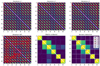 |
Fig. B.1 Illustration of the cross-validation algorithm used to measured the occurrence rate of the components through the correlation matrix MR of the vectors. The colour scale is arbitrary. Six vectors with different periods, P, (from 10 to 60 days by steps of 10 days) and ten different amplitudes were used to simulate the typical output of a PCA algorithm. The 6 ⋅ (10 + 1) = 66 components therefore produce a 66 × 66 correlation matrix, MR. The signals at longest periods (component 4, 5 and 6) start to be collinear due to the baseline of the observations (60 days). Top row: first iterations of the ordering algorithm. Bottom left: final chain as detected by the ranking algorithm. Bottom middle: same as top left after the correlation matrix has been reordered. Bottom right: border detection as given by the borders algorithm. Each cluster is clearly detected and contains a single primary components, P, (colour dots). The occurrence rate, r, of all the components are 100% in that case. The borders (vertical and horizontal white lines) can be used to define a smaller matrix R′ (here 6 × 6) which can be reordered iteratively in case of bad chain ordering which did not happened in that simulation. |
We recall that any stationary RV signal with an amplitude larger than 5 m s−1 is pre-fitted by a Keplerian solution and re- moved by YARARA, since such signals can easily be recovered on an ultra stable echelle spectrograph like HARPS. Moreover, for stars intensively observed and bright which are the main targets of our work, photon-noise and instrumental systematics are usually below 1 m s−1 on HARPS, as demonstrated in Cretignier et al. (2021). Finally, for slow rotating-stars with v sin i ≤ 3 km s−1, the RV amplitude measured by SOAP 2.0 simulations are smaller than 5 m s−1 for reasonable size of active regions (Dumusque et al. 2014). For that reason, the RV error affecting the spectra that will be used to create the master spectrum will usually not exceed 5 m s−1, a value confirmed on α Cen B (Dumusque 2018) and on the Sun (Dumusque et al. 2021).
Because residual RV shifts will usually not exceed a few m s−1, a well suited data set to evaluate the impact of residual RV shifts on the master spectrum and on our shell framework is the one of HD 10700 with the 3 m s−1 and 2 m s−1 planetary sig- nals injected (see Sect. 4.1). Thus, we perform our master spectrum construction and our shell decomposition once again on this dataset, except that this time we do not RV-shifted the spec- tra to cancel the measured CCF RVs. The obtained master spec- trum will therefore be affected by the small RV residual shifts. Performing the shell decomposition, we find that this imperfect master spectrum has no impact on the algorithm. The same shells and the same RV residuals are obtained. This can be understood by the small errors introduced on the master spectrum, at most a few m s−1 compared to the average FWHM of a spectral line on HARPS, ~6 km s−1, are three orders of magnitude greater.
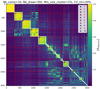 |
Fig. B.2 Illustration of the cross-validation algorithm based on the correlation matrix of the ten shells of HD 10700 (vertical and horizontal red lines). Only the first four shells are detected with an occurrence rate r >95%, whereas only the five first shell are not compatible with a single outlier explanation (r > 80%). |
Appendix C Noise injection implementation
Since photon noise follows a Poissonian distribution, the related uncertainty, σγ, is given as the square root of the flux F. The S/Ncont of a spectrum is therefore given by 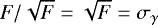 . In particular, YARARA gives output spectra that are continuum- normalised, which means that the spectra have been divided by their flux in the continuum. In this case, the photon noise in a normalised spectrum is given by
  . In a single-observation normalised spectrum, the uncertainties in flux are dominated by the photon noise and thus the S∕Ncont of a continuum normalised spectrum is simply the inverse of the flux uncertainty in the continuum. This flux uncer- tainty can either be estimated by the error bars or by measuring 1.48 times the MAD6 in YARARA river diagram maps, considering that the river diagram maps are free of all systematics.
We note that in the case of YARARA, each spectrum is ob- tained by binning all the available spectra within a night. For a star with usual moderate S∕Ncont values and a few observa- tions per night, the noise in the continuum of a nightly-binned YARARA spectrum is photon-noise dominated, and thus, if all spectra within a night have the same S∕Ncont, the S∕Ncont of the nightly binned spectrum should be in theory S/N . This theoretical value should be equal to the inverse of 1.48 times the MAD measured in YARARA river diagram maps. In the case of very bright targets, such as HD 128621, where each in- dividual observation is at S/Ncont ≥ 400 and dozens of observations are taken within a night, the noise in a nightly-binned YARARA spectrum is flat-field limited; this is because all the spectra within a night are reduced using the same flat field, which on HARPS has a S/Ncont ~ 650. Considering 20 spec- tra of HD 128621 at S/Ncont = 400, we should arrive at a theo- retical S∕Ncont of ~ 1800 for the nightly-binned spectrum if we only consider photon-noise. However, when taking the inverse of 1.48 times the MAD in the continuum of the binned spectrum, we only reach a S∕Ncont value of ~ 600, compatible with the flat-field S∕Ncont, thus demonstrating that the noise in HD 128621 YARARA spectra are flat-field dominated.
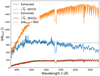 |
Fig. C.1 Examples of computed S/N |

To determine the photon noise of a nightly-binned YARARA spectrum as a function of wavelength σobs (λ), or equivalently S/N , we assume that the noise in the continuum is a smooth function of the wavelength. Indeed, even though the S∕Ncont of an observed spectrum naturally change from blue to red due to several factors, as for example: i) the stellar spectral energy distribution; ii) the atmospheric extinction; iii) the use of optical fibres; and iv) the CCD response, all those effects only introduce a slow chromatic variation. We therefore consider that 1.48 × MAD of the YARARA river diagram maps in a window7 of ± 2.5 Å around λ0 as a direct measurement of σobs(λ0). The chromatic S∕Ncont value of an observation S/N
 is thus obtained by taking the inverse value of 1.48 times a rolling MAD with the same window size. We see in Fig. C.1, that in the case of spectra that are limited by photon noise, our estimation of S∕Ncont using a rolling MAD on the YARARA river diagram maps (green curve) gives similar results as the theoretical value (red curve). However, in the case of spectra for which the noise is flat-field dominated, our estimation of S∕Ncont saturates at ~650 (blue curve) while the theoretical S∕Ncont value due tophoton-noise only is much higher (orange curve).
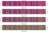 |
Fig. C.2 Examples of noise injections around the Hα = 6562.79 Åline on the spectra time series of HD 128621 (YARARA uncorrected)for different S∕Ncont values. Fromtop to bottom: S∕Ncont = 592 (nominal median values of the observations), 250, 150, and 50. This example also illustrates the approximated required S∕Ncont to detect and correct for the systematics using YARARA. For instance, at S∕Ncont=50, the pattern of interference and the Hα chromospheric variation are not detected whereas some of the telluric lines in that wavelength range are still visible. |
In Sect. 4.2.2, we tested how our shell framework was able to mitigate stellar activity for different S∕Ncont level. To be able to obtain different S∕Ncont level from YARARA spectra, we note that lowering the S∕Ncont of a spectrum by a factor x = (S/Ncont)∕(S/N , implies an increase in the photon noise by a factor of x. As a YARARA spectrum already contains some noise σobs, to reach a photon noise σsim = σobs × x we only have to add as noise σadd to the spectrum:
![\begin{eqnarray*}\sigma_{add} &=& \sqrt{\sigma_{sim}^2 - \sigma_{obs}^2} = \sigma_{obs}\sqrt{x^2 - 1} \nonumber \\&=& \sigma_{obs}\sqrt{\left[\frac{S/N_{cont}}{S/N_{cont}^{sim}}\right]^2 - 1}.\end{eqnarray*}](/articles/aa/full_html/2022/03/aa42435-21/aa42435-21-eq33.png) (C.1)
(C.1)
We decided for the noise injections to produce ’white’ pho- ton noise, which means that the same S/Ncont value was injected for all the wavelengths opposite to real observations on an in- strument which are chromatic (see Fig. C.1). For all the noise injections, the same seed of the random generator was used and only the amplitude of the noise vector was changed. An example of the river diagram of HD 128621 (systematics uncorrected by YARARA) is displayed in Fig. C.2 for three S/N realisations (250, 150, and 50) around the Hα line.
References
- Aigrain, S., Pont, F., & Zucker, S. 2012, MNRAS, 419, 3147 [NASA ADS] [CrossRef] [Google Scholar]
- Baranne, A., Queloz, D., Mayor, M., et al. 1996, A&AS, 119, 373 [NASA ADS] [CrossRef] [EDP Sciences] [Google Scholar]
- Barnes, J. R., Jeffers, S. V., Anglada-Escudé, G., et al. 2017, MNRAS, 466, 1733 [NASA ADS] [CrossRef] [Google Scholar]
- Basri, G., Wilcots, E., & Stout, N. 1989, PASP, 101, 528 [NASA ADS] [CrossRef] [Google Scholar]
- Boisse, I., Bouchy, F., Hébrard, G., et al. 2011, A&A, 528, A4 [NASA ADS] [CrossRef] [EDP Sciences] [Google Scholar]
- Borgniet, S., Meunier, N., & Lagrange, A.-M. 2015, A&A, 581, A133 [NASA ADS] [CrossRef] [EDP Sciences] [Google Scholar]
- Bouchy, F., Pepe, F., & Queloz, D. 2001, A&A, 374, 733 [NASA ADS] [CrossRef] [EDP Sciences] [Google Scholar]
- Brewer, J. M., Fischer, D. A., Blackman, R. T., et al. 2020, AJ, 160, 67 [NASA ADS] [CrossRef] [Google Scholar]
- Collier Cameron, A., Mortier, A., Phillips, D., et al. 2019, MNRAS, 487, 1082 [Google Scholar]
- Collier Cameron, A., Ford, E. B., Shahaf, S., et al. 2021, MNRAS, 505, 1699 [NASA ADS] [CrossRef] [Google Scholar]
- Cosentino, R., Lovis, C., Pepe, F., et al. 2012, in Proc. SPIE, 8446, Ground-based and Airborne Instrumentation for Astronomy IV, 84461V [NASA ADS] [CrossRef] [Google Scholar]
- Cretignier, M., Dumusque, X., Allart, R., Pepe, F., & Lovis, C. 2020a, A&A, 633, A76 [NASA ADS] [CrossRef] [EDP Sciences] [Google Scholar]
- Cretignier, M., Francfort, J., Dumusque, X., Allart, R., & Pepe, F. 2020b, A&A, 640, A42 [NASA ADS] [CrossRef] [EDP Sciences] [Google Scholar]
- Cretignier, M., Dumusque, X., Hara, N. C., & Pepe, F. 2021, A&A, 653, A43 [NASA ADS] [CrossRef] [EDP Sciences] [Google Scholar]
- Davis, A. B., Cisewski, J., Dumusque, X., Fischer, D. A., & Ford, E. B. 2017, ApJ, 846, 59 [NASA ADS] [CrossRef] [Google Scholar]
- de Beurs, Z. L., Vanderburg, A., Shallue, C. J., et al. 2020, AJ, submitted [arXiv:2011.00003] [Google Scholar]
- Demory, B.-O., Ehrenreich, D., Queloz, D., et al. 2015, MNRAS, 450, 2043 [CrossRef] [Google Scholar]
- Donati, J.-F., Yu, L., Moutou, C., et al. 2017, MNRAS, 465, 3343 [NASA ADS] [CrossRef] [Google Scholar]
- Dumusque, X. 2012, Ph.D. thesis, Observatory of Geneva [Google Scholar]
- Dumusque, X. 2018, A&A, 620, A47 [NASA ADS] [CrossRef] [EDP Sciences] [Google Scholar]
- Dumusque, X., Lovis, C., Ségransan, D., et al. 2011a, A&A, 535, A55 [NASA ADS] [CrossRef] [EDP Sciences] [Google Scholar]
- Dumusque, X., Udry, S., Lovis, C., Santos, N. C., & Monteiro, M. J. P. F. G. 2011b, A&A, 525, A140 [NASA ADS] [CrossRef] [EDP Sciences] [Google Scholar]
- Dumusque, X., Pepe, F., Lovis, C., et al. 2012, Nature, 491, 207 [Google Scholar]
- Dumusque, X., Boisse, I., & Santos, N. C. 2014, ApJ, 796, 132 [NASA ADS] [CrossRef] [Google Scholar]
- Dumusque, X., Cretignier, M., Sosnowska, D., et al. 2021, A&A, 648, A103 [NASA ADS] [CrossRef] [EDP Sciences] [Google Scholar]
- Feng, F., Tuomi, M., Jones, H. R. A., et al. 2017, AJ, 154, 135 [Google Scholar]
- Figueira, P., Santos, N. C., Pepe, F., Lovis, C., & Nardetto, N. 2013, A&A, 557, A93 [NASA ADS] [CrossRef] [EDP Sciences] [Google Scholar]
- Fischer, D. A., Anglada-Escude, G., Arriagada, P., et al. 2016, PASP, 128, 066001 [Google Scholar]
- Gupta, A. F., Wright, J. T., Robertson, P., et al. 2021, AJ, 161, 130 [NASA ADS] [CrossRef] [Google Scholar]
- Hall, R. D., Thompson, S. J., Handley, W., & Queloz, D. 2018, MNRAS, 479, 2968 [NASA ADS] [CrossRef] [Google Scholar]
- Hatzes, A. P. 2013, ApJ, 770, 133 [NASA ADS] [CrossRef] [Google Scholar]
- Huélamo, N., Figueira, P., Bonfils, X., et al. 2008, A&A, 489, L9 [NASA ADS] [CrossRef] [EDP Sciences] [Google Scholar]
- Jurgenson, C., Fischer, D., McCracken, T., et al. 2016, in SPIE Conf. Ser., 9908, 99086T [Google Scholar]
- Lanza, A. F., Malavolta, L., Benatti, S., et al. 2018, A&A, 616, A155 [NASA ADS] [CrossRef] [EDP Sciences] [Google Scholar]
- Lienhard, F., & Mortier, A. 2021, in The 20.5th Cambridge Workshop on Cool Stars, Stellar Systems, and the Sun (CS20.5), 155 [Google Scholar]
- Lisogorskyi, M., Jones, H. R. A., Feng, F., Butler, R. P., & Vogt, S. 2021, MNRAS, 500, 548 [Google Scholar]
- Löhner-Böttcher, J., Schmidt, W., Schlichenmaier, R., Steinmetz, T., & Holzwarth, R. 2019, A&A, 624, A57 [Google Scholar]
- Marchwinski, R. C., Mahadevan, S., Robertson, P., Ramsey, L., & Harder, J. 2015, ApJ, 798, 63 [Google Scholar]
- Mayor, M., Pepe, F., Queloz, D., et al. 2003, The Messenger, 114, 20 [NASA ADS] [Google Scholar]
- Meunier, N., Desort, M., & Lagrange, A.-M. 2010, A&A, 512, A39 [NASA ADS] [CrossRef] [EDP Sciences] [Google Scholar]
- Meunier, N., Lagrange, A.-M., Borgniet, S., & Rieutord, M. 2015, A&A, 583, A118 [NASA ADS] [CrossRef] [EDP Sciences] [Google Scholar]
- Milbourne, T. W., Haywood, R. D., Phillips, D. F., et al. 2019, ApJ, 874, 107 [Google Scholar]
- Milbourne, T. W., Phillips, D. F., Langellier, N., et al. 2021, ApJ, 920, 21 [NASA ADS] [CrossRef] [Google Scholar]
- Pandas development team, T. 2020, pandas-dev/pandas: Pandas [Google Scholar]
- Pepe, F., Mayor, M., Galland, F., et al. 2002, A&A, 388, 632 [NASA ADS] [CrossRef] [EDP Sciences] [Google Scholar]
- Pepe, F., Cristiani, S., Rebolo, R., et al. 2021, A&A, 645, A96 [NASA ADS] [CrossRef] [EDP Sciences] [Google Scholar]
- Rajpaul, V., Aigrain, S., Osborne, M. A., Reece, S., & Roberts, S. 2015, MNRAS, 452, 2269 [Google Scholar]
- Rajpaul, V., Aigrain, S., & Roberts, S. 2016, MNRAS, 456, L6 [NASA ADS] [CrossRef] [Google Scholar]
- Reiners, A., Shulyak, D., Anglada-Escudé, G., et al. 2013, A&A, 552, A103 [NASA ADS] [CrossRef] [EDP Sciences] [Google Scholar]
- Reiners, A., Mrotzek, N., Lemke, U., Hinrichs, J., & Reinsch, K. 2016, A&A, 587, A65 [NASA ADS] [CrossRef] [EDP Sciences] [Google Scholar]
- Saar, S. H. 2009, in American Institute of Physics Conference Series, Vol. 1094, 15th Cambridge Workshop on Cool Stars, Stellar Systems, and the Sun, ed. E. Stempels, 152 [NASA ADS] [Google Scholar]
- Saar, S. H., & Donahue, R. A. 1997, ApJ, 485, 319 [Google Scholar]
- Simola, U., Dumusque, X., & Cisewski-Kehe, J. 2019, A&A, 622, A131 [NASA ADS] [CrossRef] [EDP Sciences] [Google Scholar]
- Suárez Mascareño, A., Faria, J. P., Figueira, P., et al. 2020, A&A, 639, A77 [Google Scholar]
- Thompson, S. J., Queloz, D., Baraffe, I., et al. 2016, in SPIE Conf. Ser., 9908, 99086F [Google Scholar]
- Thompson, A. P. G., Watson, C. A., de Mooij, E. J. W., & Jess, D. B. 2017, MNRAS, 468, L16 [NASA ADS] [CrossRef] [Google Scholar]
- VanderPlas, J. T. 2018, ApJS, 236, 16 [Google Scholar]
- Wes McKinney. 2010, in Proceedings of the 9th Python in Science Conference, eds. S. van der Walt & J. Millman, 56 [CrossRef] [Google Scholar]
- Wise, A. W., Dodson-Robinson, S. E., Bevenour, K., & Provini, A. 2018, AJ, 156, 180 [NASA ADS] [CrossRef] [Google Scholar]
- Zechmeister, M., Reiners, A., Amado, P. J., et al. 2018, A&A, 609, A12 [NASA ADS] [CrossRef] [EDP Sciences] [Google Scholar]
- Zechmeister, M., Reiners, A., Amado, P. J., et al. 2020, SERVAL: SpEctrum Radial Velocity AnaLyser Astrophysics Source Code Library, [record ascl:2006.011] [Google Scholar]
- Zhu, W., & Dong, S. 2021, ARA&A, 59, 291 [NASA ADS] [CrossRef] [Google Scholar]
All Figures
|
Fig. 1 Projection of a small part of a spectrum into the (df0∕dλ, f, δf) space that we call the shell space. Top: reference spectrum used to perform the change of variables (in black). The coloured dots correspond to the value of δf when comparing a Doppler shifted spectrum to the reference spectrum. Bottom: projection of the Doppler shifted spectrum onto the shell space. Each point in this new space corresponds to an original point of the reference spectrum and the colour coding corresponds, as above, to the value of δf when comparing a Doppler shifted spectrum to the reference spectrum. Positions of the lines’ cores were indexed to make the identification easier. The mean velocity difference between the shifted and reference spectra δv can be recovered as the slope between the flux gradient and δf. |
| In the text | |
|
Fig. 2 Projection of the Doppler shifted spectrum onto the shell space for a real spectrum of HD 10700. The shell space has been dividedin a 9 × 9 grid (black lines) to increase the S/N of the raw shell after binning all the points within each cell. |
| In the text | |
|
Fig. 3 Shell representation and statistics of a spectrum from HD 10700. Here, we highlight the fraction of spectral elements that fall within each bin, as well as their average wavelength (in colour scale). |
| In the text | |
|
Fig. 4 Shell decomposition of HD 10700 spectra. Left: representation of the different shells basis components and the time series of the coefficients αj(t) in fronteach of those shell basis components when modelling the RVs of HD 10700 (see Eq. (4)). All the components are orthogonal to the Doppler shell basis component (DS) displayed at the bottom (similar to Fig. 2) thanks to a Gram–Schimdt algorithm. The pixel grid in the shell space on which the PCA was trained (dots) is shown, as well as a smooth function interpolated on the full shell space using a cubic interpolation algorithm. Middle: generalised Lomb–Scargle periodogram of the αj (t) shell component coefficients. The 0.1% false alarm probability (FAP) level for each periodogram is indicated by an horizontal dotted-dashed line. From top to bottom, we can see the five first principal shell basis components and the DS. The Pearsoncorrelation coefficient between the αj(t) and the CCF RV time series is indicated on the right side of each subplot. The lowest periodogram represents the RV time series linearly decorrelated from the αj coefficients (similar to Eq. (5)). The power at the planetary injected periods (vertical red lines) is never the dominant power for any shell. This is particularly true for the 37-day signal less significant than the 0.1% FAP level. Some power is observed around 122 days for PS1 and PS4 due to an alias of a one-year systematics (see main text). Right: explained variance curve of the PCA components. Our cross-validation algorithm (see Appendix A) provides four significant components (> 95%). The components compatible with a single outlier explanation (<80%) are shown in red. |
| In the text | |
|
Fig. 5 Measurement of the collinearity between planets in circular orbits and the αj (t) basis for HD 10700. The simulations are made of 18 different phases and 15 000 different periods. The envelope describes the 1-sigma dispersion obtained from the different phases for the same period. The injected planets are marked by vertical lines. A typical decrease of 2 ± 1 and 7 ± 4% can be expected for the 37-day and 122-day planets, respectively. Those results are coherent with the ~ 2 m s−1 and ~ 2.85 m s−1 planetary signals recovered, while the original signals injected for those planets was 2 and 3 m s−1, respectively. |
| In the text | |
|
Fig. 6 Polar periodogram for the 2010 HD 128621 dataset obtained for a fixed period of 36 days, known to be the stellar rotation period of HD 128621. Each dot represents a spectral line. Peculiar activity proxies and αj (t) coefficient time series are shown as markers of different types (see legend). The radial coordinate is the weighted |
| In the text | |
|
Fig. 7 Polar periodogram for the 2011 and 2012 HD 128621 datasets after YARARA correction. For 2012, the highest peaks in the periodogram correspond to a period of 40 days, so we display the polar periodogram at 40 days rather than36 days. A clear time-lag between the RV variation of each line and the CaII H&K (purple cross) of ϕ ~ 90° (9 days) and ϕ ~ 45° (5 days) is visible in 2011 and 2012, respectively. The RVs are however in phase with the multi-linear model of αj (pink square) as well as with the CCF FWHM (orange star). |
| In the text | |
|
Fig. 8 Shell decomposition of HD 128621 spectra. The first shell is the one presenting the highest correlation with CCF RVs. The second shell is similar to a change of the line bisector and the time series of the related coefficient strongly correlated with the VSPAN of the CCF. Third shell, present mostly power at one-year and a half-year and is more related to instrumental systematics. The fourth component (fifth one according to the explained variance) seems once again to be related to stellar activity. The next components all possess a score lower than 80% and are therefore considered as less significant. After the decorrelation by the shell coefficients αj (t), the planetary injected period at 54 days (vertical red line) becomes the dominant signal, with the other peaks at 47 and 63 days being the one-year aliases. |
| In the text | |
|
Fig. 9 Measurement of the collinearity between planets in circular orbits and the αj (t) basis for HD128621. A maximum of absorption of 25 ± 5% is observed for the rotational period of the star at 39 days. It demonstrates than even if the rotational signal is strongly mitigated, a real circular planetary signal at 39-days would not have been more absorbed than this. For the injected planetary signal at 54 days, the absorption is 3 ± 2%. Absorption at one-year and a half-year are also noticeable. |
| In the text | |
|
Fig. 10 Correlation matrix of the CCF RVs time series, v(t), the shell basis coefficients, αj(t), and the full model fitted with other common activity proxies. The different shells basis coefficients show weak correlations with the CCF moments highlighting an indirect connection between shells and CCFs. |
| In the text | |
|
Fig. 11 Periodograms of the residuals RVs parametrised by the model complexity (name convention as in Eq. (5)). All the periodograms are normalised according to their respective 1% FAP level (horizontal dotted-dashed line). The RV rms of the residuals for each model is indicated in the legend as well as the integrated power between 32 and 45 days. Top: results obtained by increasingly adding shell basis coefficients into the multi-linear model of Eq. (5). Once three shell basis coefficients are fitted, the rotational period is no more significant (green and red). Bottom: comparison between the residuals obtained after fitting for four shell basis coefficients (red) or the three classical CCF moments (FWHM, VSPAN and contrast) plus the CaII H&K. Both CCF moments before (CCFY 0, blue) and after YARARA processing (CCFY 1, green) were used. |
| In the text | |
|
Fig. 12 Inverse projection of the four significant PCA shell basis components, shown on the left of Fig. 8, used to correct the RV time series of α Cen B. The inverse projection was realised for Gaussian line profiles at 5250 Å with a FWHM equivalent to 6 km s−1 and threedifferent line depths (0.2, 0.45, and 0.7, from top to bottom). The delta flux variations, δf, evaluated along the line profile chord (see Fig. 1) are indicated after magnification above the Gaussian line profile and compared with δf = 0 (horizontal dotted line). The bisector of each line profile is also indicated after magnification and compared to the initial Gaussian profile (vertical dotted lines). |
| In the text | |
|
Fig. 13 Noise injection tests performed on HD 128621 to evaluate the performance of our shell framework in mitigating stellar activity depending on the continuum signal-to-noise ratio, S∕Ncont. The cross-validation algorithm to select only shell basis components with significant variance was disabled and five componentswere used for the fitted model. Top left: correlation between the noise-affected shell basis coefficients αj and their respective coefficients without extra-noise injected αj,obs. A shell basis component can be considered as recovered once its related coefficient αj exceeds a correlation value with αj,obs higher than |
| In the text | |
|
Fig. 14 Noise injection tests performed on HD 128621 to evaluate the performance of our shell framework in mitigating stellar activity. In this figure, we show the dependence between the integrated power of signals between 32 and 45 days, which contain mostly stellar activity signal, and the S∕Ncont. Previous values mentioned in Fig. 11 and obtained at observed S∕Ncont values (~650) are reported (solid horizontal lines). Activating the cross-validation algorithm to select only shell basis component with significant signal and imposing the S∕N > 1 criterion to reject noisy shell elements allow to mitigate significantly stellar activity starting at a S∕Ncont = 200 (orange curve) instead of S∕Ncont = 250 (blue curve). One thousand random realisations of white noise with the time samplingof the data were produced to get a reference power value, given at ± 1σ (gray area). |
| In the text | |
|
Fig. B.1 Illustration of the cross-validation algorithm used to measured the occurrence rate of the components through the correlation matrix MR of the vectors. The colour scale is arbitrary. Six vectors with different periods, P, (from 10 to 60 days by steps of 10 days) and ten different amplitudes were used to simulate the typical output of a PCA algorithm. The 6 ⋅ (10 + 1) = 66 components therefore produce a 66 × 66 correlation matrix, MR. The signals at longest periods (component 4, 5 and 6) start to be collinear due to the baseline of the observations (60 days). Top row: first iterations of the ordering algorithm. Bottom left: final chain as detected by the ranking algorithm. Bottom middle: same as top left after the correlation matrix has been reordered. Bottom right: border detection as given by the borders algorithm. Each cluster is clearly detected and contains a single primary components, P, (colour dots). The occurrence rate, r, of all the components are 100% in that case. The borders (vertical and horizontal white lines) can be used to define a smaller matrix R′ (here 6 × 6) which can be reordered iteratively in case of bad chain ordering which did not happened in that simulation. |
| In the text | |
|
Fig. B.2 Illustration of the cross-validation algorithm based on the correlation matrix of the ten shells of HD 10700 (vertical and horizontal red lines). Only the first four shells are detected with an occurrence rate r >95%, whereas only the five first shell are not compatible with a single outlier explanation (r > 80%). |
| In the text | |
|
Fig. C.1 Examples of computed S/N |
| In the text | |
|
Fig. C.2 Examples of noise injections around the Hα = 6562.79 Åline on the spectra time series of HD 128621 (YARARA uncorrected)for different S∕Ncont values. Fromtop to bottom: S∕Ncont = 592 (nominal median values of the observations), 250, 150, and 50. This example also illustrates the approximated required S∕Ncont to detect and correct for the systematics using YARARA. For instance, at S∕Ncont=50, the pattern of interference and the Hα chromospheric variation are not detected whereas some of the telluric lines in that wavelength range are still visible. |
| In the text | |
Current usage metrics show cumulative count of Article Views (full-text article views including HTML views, PDF and ePub downloads, according to the available data) and Abstracts Views on Vision4Press platform.
Data correspond to usage on the plateform after 2015. The current usage metrics is available 48-96 hours after online publication and is updated daily on week days.
Initial download of the metrics may take a while.