| Issue |
A&A
Volume 659, March 2022
|
|
|---|---|---|
| Article Number | A199 | |
| Number of page(s) | 20 | |
| Section | Numerical methods and codes | |
| DOI | https://doi.org/10.1051/0004-6361/202141480 | |
| Published online | 29 March 2022 | |
SUPPNet: Neural network for stellar spectrum normalisation⋆
1
Astronomical Institute, University of Wrocław, Kopernika 11, 51-622 Wrocław, Poland
e-mail: tomasz.rozanski@uwr.edu.pl
2
Department of Computer Science, Faculty of Fundamental Problems of Technology, Wrocław University of Science and Technology, Wrocław, Poland
3
Faculty of Electronics, Wrocław University of Science and Technology, Wrocław, Poland
Received:
6
June
2021
Accepted:
9
December
2021
Context. Precise continuum normalisation of merged échelle spectra is a demanding task that is necessary for various detailed spectroscopic analyses. Automatic methods have limited effectiveness due to the variety of features present in the spectra of stars. This complexity often leads to the necessity for manual normalisation which is highly time-consuming.
Aims. The aim of this work is to develop a fully automated normalisation tool that works with order-merged spectra and offers flexible manual fine-tuning, if necessary.
Methods. The core of the proposed method uses the novel, fully convolutional deep neural network (SUPP Network) that was trained to predict a pseudo-continuum. The post-processing step uses smoothing splines that give access to regressed knots, which are useful for optional manual corrections. The active learning technique was applied to deal with possible biases that may arise from training with synthetic spectra and to extend the applicability of the proposed method to features absent in this kind of spectra.
Results. The developed normalisation method was tested with high-resolution spectra of stars with spectral types from O to G, and gives a root mean squared (RMS) error over the set of test stars equal to 0.0128 in the spectral range from 3900 Å to 7000 Å and 0.0081 in the range from 4200 Å to 7000 Å. Experiments with synthetic spectra give a RMS of the order of 0.0050.
Conclusions. The proposed method leads to results that are comparable to careful manual normalisation. Additionally, this approach is general and can be used in other fields of astronomy where background modelling or trend removal is a part of data processing.
Key words: techniques: spectroscopic / methods: numerical / stars: general / line: profiles
The algorithm is available online: https://git.io/JqJhf.
© ESO 2022
1. Introduction
Electromagnetic spectra of astronomical objects such as stars, galaxies, and exoplanets are a very abundant source of information and enable us to study the physics of the objects in detail. Low-resolution spectra are closely related to photometry and can be used to determine the basic properties of stars, such as effective temperatures, surface gravities, and metallicities. High-resolution spectra allow us to investigate profiles of separate absorption and emission lines in detail, and make it possible to measure individual abundances of elements, understand the vertical structure of a stellar atmosphere, and study its velocity fields (e.g. microturbulence, macroturbulence, rotation, stellar oscillations, and granulation).
The continuum-normalisation process is an important part of spectrum preprocessing, because for the next steps of the analysis, in general, the pseudo-continuum should be correctly subtracted. The problem of continuum normalisation is non-trivial, as several factors are responsible for the shape of a spectrum, including the real stellar continuum shape, the Earth atmosphere, the characteristics of optical and electronic components of a spectrograph, the presence of cosmic rays, and last but not least, residuals introduced by pipelines used by observatories to calibrate and reduce spectra. These residuals are usually a result of imperfect order merging and blaze function removal. Several existing normalisation methods are worth mentioning, such as filtering methods (moving window maximum filtering, asymmetric sigma clipping, etc.), and low-order polynomial fitting, smoothing in the frequency domain, and methods based on the concept of convex-hull and alpha-shape theories (Xu et al. 2019; Cretignier et al. 2020). These all try to remove spectral lines from the spectrum and then fit a low-order polynomial or spline function to the remaining pseudo-continuum, and they all contain some free parameters that need to be adjusted manually. For a broad overview of methods and problems present in the normalisation of stellar spectra we recommend the article by Cretignier et al. (2020).
Normalisation methods based on polynomial fitting and frequency domain filtering suffer from the trade-off between the treatment of rapidly changing parts of a continuum (e.g. ripples often present in merged échelle spectra) and the presence of wide spectral features (e.g. hydrogen lines or molecular bands). These limitations can be partially overcome by introducing some adaptive penalised least-squares terms in the minimisation objective. This approach is extensively used in the field of Raman spectroscopy (Cadusch et al. 2013). Methods based on the concept of convex hulls also have some limitations. They assume that the local maximum is a good indicator of a stellar continuum. In most cases, this is a reasonable attitude, but breaks for spectra with emission features present and in regions with extensively blended lines, where the continuum is well above the measured spectrum (e.g. in the optical spectra of G or later stars). All these methods share the problem that features located in regions covered with spectral lines are lost. This does not allow for the effective recovery of the pseudo-continuum shape in the parts of spectra mentioned above. The continuum in these parts is only smoothed to match the surroundings of the line. Additionally, those methods are particularly sensitive to the level of noise, the projected rotational velocity, and the resolution of the instrument used to observe the spectra.
These limitations can be overcome when we have a template for a given spectrum. Normalisation can then be reduced to dividing the spectrum by the model and then using the selected trend-fitting tool –for example adaptive spline functions– to model a pseudo-continuum. In this case, the challenge is to successfully find a model for the spectrum, the parameters of which are unknown at the first stage of the analysis. In turn, the proposed approach, utilising information from the entire spectrum including parts covered with spectral lines, is resistant to the above-mentioned problems and can be used in a fully automatic manner, offering, at the same time, the flexibility of manual corrections, if necessary.
Nonetheless, an astronomer experienced in spectrum normalisation is able to fit a pseudo-continuum taking most of the complexities into account, especially when normalisation is done iteratively during model fitting. One of the tools that make the fully manual continuum fitting and initial stellar parameter estimation straightforward is the application HANDY1. However, manual normalisation has several important drawbacks. It is very time-consuming, prone to human biases, and is not reproducible. The manual normalisation cannot be done reliably in regions covered by wide lines and line blends when synthetic spectra are not used as a reference. Manual normalisation strengths suggest that the key points are the understanding of a spectrum and the experience with features that may appear in the pseudo-continuum. These findings suggest that machine learning algorithms are promising tools for overcoming the mentioned limitations.
The use of machine learning algorithms is becoming increasingly frequent in the physical sciences (Carleo et al. 2019), including astronomy (Ball & Brunner 2010; Baron 2019), and has become possible in recent years thanks to important developments in the algorithms of machine learning, especially in the neural network field, and the constant and rapid increase of available computational power. On the other hand, astronomy is delivering increasingly numerous and complex astrometric (e.g. Gaia mission Gaia Collaboration 2016), photometric (e.g. Zwicky Transient Facility and future Vera Rubin Observatory with Legacy Survey of Space and Time Mahabal et al. 2019; Ivezić et al. 2019) and spectroscopic (e.g. ESO database2; APOGEE, Majewski et al. 2017; LAMOST, Zhao et al. 2012) databases, which are also growing in size rapidly. Machine learning has already been applied in various tasks in the field of astronomy; for example, real-time detection of gravitational waves and parameter estimation (George & Huerta 2018), estimation of effective temperatures and metallicities of M-type stars (Antoniadis-Karnavas et al. 2020), estimation of initial parameters for asteroseismic modelling (Hendriks & Aerts 2019), classification of diffuse interstellar bands (Hendriks & Aerts 2019), and morphological segmentation of galaxies (Farias et al. 2020).
We explore deep artificial neural networks (DNN) in search of architectures that can deal with a pseudo-continuum prediction task. We propose a new algorithm based on the neural network SUPPNet that achieves results comparable to those of human professionals.
2. Machine learning and spectrum normalisation
To our knowledge, this is the first approach to automated stellar spectrum normalisation using tools based on deep learning. From the above examples, it is clear that the fundamental limitations of the previous methods are: an implicit assumption that a local maximum in a spectrum is a good indicator of a pseudo-continuum; the necessity for manual adjustments of several parameters; often poor results when the pseudo-continuum passes trough emission features; and ripples that arise from order merging (échelle spectra). Deep neural networks are natural candidates to overcome these limitations, as in principle they are capable of grasping complex priors and approximating any function. This means that a suitable neural network model after training on a representative dataset should learn to recognise a type of spectrum and a pseudo-continuum and be able to fit the pseudo-continuum correctly in most cases. In this approach, the quality of a spectrum normalisation algorithm is restricted by the generality and quality of an available training set.
To frame the normalisation problem in the context of deep learning, we consider spectrum normalisation as filtering from the domain of spectrum measurement to the domain of possible pseudo-continua. As a filter, and one that is flexible enough to implement such a mapping, we used a fully convolutional neural network (CNN) of novel architecture, which is mainly based on the work done in the field of computer vision, in particular in the semantic segmentation problem.
2.1. Training data description
A machine learning model can be as good as the data used for its training but not any better. For this reason, much attention was paid to the proper preparation of the training data. We applied the active learning technique, and so prepared two datasets: the first composed of synthetic spectra only, and the second based on automatically normalised and manually corrected observational spectra. We refer to supplementation of the training process with spectra and pseudo-continua from manual normalisation as active machine learning.
We started by preparing an extensive set of synthetic continuum-normalised spectra. We used SYNTHE/ATLAS (Kurucz 1970) codes to compute 10 000 spectra with randomly selected atmospheric parameters (effective temperature, Teff, ranging from 3000 K to 30 000 K and logarithm of surface gravity, log g, from 1.0 to 5.5). We also used BSTAR and OSTAR grids (Lanz & Hubeny 2003, 2007), which together span an effective temperature range from 15 000 K to 55 000 K, and logarithm of surface gravity from 1.75 to 4.75 (not in the whole range of temperatures). The main difference between these two sources of spectra is a different treatment of atomic level populations. The ATLAS code solves the classical stellar atmosphere problem, and SYNTHE computes the synthetic spectrum assuming local thermodynamic equilibrium (LTE), which means that level populations are calculated using the Boltzmann distribution and the Saha ionisation equation. In the case of BSTAR and OSTAR grids, these were calculated using SYNSPEC/TLUSTY codes that explicitly solve rate equations for a chosen set of levels. This is especially important for hotter stars, where the radiative processes dominate the collisional transitions and non-LTE effects become prominent. Including non-LTE effects leads to changes in line depths and, more importantly, the frequent appearance of emission features.
Some families of analytical functions (sinusoidal, smoothed sawtooth, Akima spline with five knots) and also some continua coming from manual normalisation were used as artificial pseudo-continua shapes. To build the first training dataset, the spectrum from the set of prepared synthetic spectra was sampled; part of it was randomly chosen. Next, this spectrum was convolved with a random broadening kernel and finally multiplied by an artificial continuum. Repeating this procedure about 150 000 times led to the production of a large set composed of diverse training samples. The broadening kernel included rotation, macroturbulence, and instrumental broadening. Rotation and macroturbulence velocities were chosen randomly in physically reasonable ranges. A projected rotation velocity (v sin i) range depends on effective temperature and is drawn from a uniform distribution with the lower boundary equal to zero, and the upper one successively equal to 50, 100, 200, 300, and 400 km s−1 in the ranges (< 5000), (5000, 6000), (6000, 7500), (7500, 10 000), and (> 10 000) K, respectively. This distribution is based on the discussion presented by Royer (2009). The macroturbulence velocity, ζv, was drawn from the same uniform distribution in the range from 0 to 30 km s−1, regardless of effective temperature. The chosen instrumental resolution (from 40 000 to 120 000) covers a range of the most available high-resolution spectrographs.
The second stage of learning used the training set extended by the active dataset, which is composed of automatically normalised and manually corrected observational spectra (application and description of active learning in an astronomical context can be found in the work by Škoda et al. 2020). First, the model trained on synthetic data was used to normalise spectra from UVES Paranal Observatory Project UVES POP3; Bagnulo et al. 2003; IC 2391, NGC 6475, and the brightest stars of southern sky, resolution equal to 80 000, and the set of FEROS4 spectra (153 spectra with a signal-to-noise ratio (S/N) > 500 without object duplicates, and resolution equal to 48 000). Normalisation was then manually checked and carefully corrected for each automatically processed spectrum. This resulted in a set of around 250 normalised spectra and pseudo-continua fits, making up the active dataset.
2.2. Tasks description
Initial tests of deep learning methods in stellar spectrum processing focused on two distinct tasks: segmentation of spectra into pseudo-continuum and non-pseudo-continuum parts, and pseudo-continuum prediction. The segmentation can be considered as a subclass of a classification problem, and is designed to predict the class that a segment of input data belongs to. The segment can be as small as one pixel in the case of image segmentation or a flux measurement at a given wavelength (sample) in the case of one-dimensional spectral data segmentation. In our case, we classify spectra sample-wise into two classes: ‘continuum’, and ‘non-continuum’ (see the bottom panel of Fig. 1 for an example).
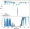 |
Fig. 1. Result of HD 27411 (A3m) spectrum processing. Left upper panel: the spectrum and the predicted continuum near the Hα line. Lower left panel: the corresponding segmentation mask. The shaded area denotes the estimated uncertainty. |
Segmentation can be given by a function f : ℛn → {0, 1}n, where n ∈ 𝒩, is the number of samples in the input and the output, 1 corresponds to the pseudo-continuum class, and 0 to the non-pseudo-continuum class. It is important to note that the result returned by the last layer of a neural network is composed of real numbers in the range from 0 to 1. Thresholding must be applied to obtain discrete classes. The common choice used also in this work is 0.5. Spectrum segmentation was considered here as an auxiliary task and as a potential regularisation technique (Kukačka et al. 2017).
A functional form of continuum prediction, which is a multidimensional regression, differs slightly from the segmentation and is given by f : ℛn → ℛn, with the same notation as above. The co-domain here is over the real numbers, instead of a discrete set of values that represent different classes. An exemplary result of such a prediction for both segmentation and a pseudo-continuum prediction task is given in Fig. 1.
2.3. Loss functions, metrics, and optimisers
Training a neural network requires an optimisation algorithm that finely adjusts free parameters of the model to the approximate trained function. The quality of the obtained mapping can be evaluated using various loss functions and metrics. A loss function denotes a differentiable function the value of which is optimised during the training process by the algorithm that iteratively adjusts free parameters of a neural network under the training. A metric is a function that is used to evaluate the performance of the model but is not directly used for optimisation during the training. Metric functions can be non-differentiable. The adopted naming convention comes from the TensorFlow machine learning library (Abadi et al. 2015).
The cross-entropy loss function is often used for segmentation:
where N is a number of samples, yi is a vector of target classes for i-th sample, and  is a vector of the model’s output for the same sample. yi, j equals 1 only if the ith sample belongs to jth class, so yi ∈ {0, 1}M, where M is a number of classes. The cross-entropy equals zero if a model perfectly assigns classes to samples. In this work, the binary-cross-entropy loss was applied as there are only two distinct classes. The accuracy, which is given by the number of correct predictions divided by the number of all predictions, was used as a metric. Here, in the case of the binary segmentation, the accuracy = (TP + TN)/N, where TP denotes the number of true positive predictions, TN is the number of to true negatives, and N gives the number of samples.
The mean squared error (MSE) was used as a loss function for the pseudo-continuum prediction, and is given by
where N denotes the number of samples, y is a vector of target values, and  is an estimated vector. MSE is a standard loss function for a regression problem. The mean absolute error (MAE) was used as a metric for this task. The functional form of MAE is given by
All performed experiments use the Nesterov-accelerated adaptive moment estimation optimiser (Nadam; Dozat 2016), which iteratively adjusts free parameters of a neural network during a training process. It is based on two main concepts. The first is Nesterov’s momentum, which is beneficial in dimensions of an objective function with small curvature that consistently points in one direction (Nesterov 1983). The second concept is the adaptive learning rate, which is able to compute individual learning rates based on the first and second moments of gradients (Adam; Kingma & Ba 2017), and works well with sparse gradients and non-stationary objectives.
2.4. Exploratory neural network tests
Initial exploration of neural network architectures was focused on tasks of pseudo-continuum prediction and spectrum segmentation. As these problems are inherently one-dimensional (inputs and targets are sequential data), we implemented and tested one-dimensional versions of several neural network architectures that were successfully used in the field of image segmentation. We expected that advances made in the two-dimensional domain, with necessary adaptations and some minor changes, could be adopted for the processing of one-dimensional signals such as stellar spectra. The purpose of these tests was to check this hypothesis. To some extent, the method to find the best neural network follows the work of Radosavovic et al. (2020).
The selection of potential architectures was based in particular on the paper of Hoeser & Kuenzer (2020), which gives a detailed overview of both the historical development and current state-of-the-art solutions. The architectures selected for the experiments were: fully convolutional network (FCN, Long et al. 2015), deconvolution network (DeconvNet, Noh et al. 2015), U-Net (Ronneberger et al. 2015), UNet++, (Zhou et al. 2018), feature pyramid network (FPN, Lin et al. 2017; Kirillov et al. 2019), and pyramid scene parsing network (PSPNet, Zhao et al. 2017). Additionally, a new architecture was proposed, namely UPPNet, which is an extension of the U-Net architecture.
The same training and evaluation scheme were used for all tests to make the comparison informative. Each tested neural network is composed of a body and a prediction head. The body is the part sampled from the adopted parameters space, considering the type of architecture and its free hyper-parameters (e.g. a number of layers, etc.). As input, it takes a one-dimensional spectrum (vector of the length equal to 8192) and outputs several feature maps of the same length as the input spectrum (e.g. in the case of a body that returns eight feature maps, a matrix of size 8192 × 8 is an output). In the context of a one-dimensional spectrum, feature maps can represent different shapes of spectral lines. Schematic diagrams of all tested bodies can be found in Figs. A.1–A.7. As the main building block, all networks use residual bottleneck blocks with group convolution (Xie et al. 2016), referred to here as residual blocks (RBs). Hyper-parameters of RBs are: a number of feature maps, a group width, and a bottleneck ratio (in all experiments the bottleneck ratio was fixed to one; see Radosavovic et al. 2020). The head takes feature maps from the body part as an input and returns a final prediction. All heads share the same architecture, that is, they have three point-wise convolutional layers (LeCun et al. 1989) with the number of features equal to 64, 32, followed by 1. In the first two layers, the ReLU (ReLU(x) = max(x, 0)) activation function was used, while in the third one, the softmax function is used for segmentation and ReLU for pseudo-continuum prediction. The exception is the FCN, the architecture of which does not allow for this consistent approach. In this case, we skipped some of the tests (details are given in the architecture description below).
One hundred neural architecture realisations with a number of free parameters ranging from 200 000 to 300 000 were sampled from each architecture and trained in a low-data regime (∼5000 training samples from the synthetic training dataset, 30 epochs training, where epoch means single complete pass through the training data) in a pseudo-continuum prediction task. Validation of networks was performed on the validation dataset separated from the training set at the beginning. The obtained distribution of models can be found in Fig. 2, and shows the probability that the loss value on a validation set of a neural network sampled from a given architecture will be lower than a corresponding abscissa value. For example, approximately 60% of neural networks of the UPPNet (full) architecture have a loss function value lower than 4 × 10⁻³. This plot shows that neural networks of different architectures differ in the concentration of high-quality models in their parameter space and in the mean squared error of the best neural network. The UPPNet (full) can therefore be considered the most promising architecture as it gives many relatively good models and also has the best model among all the trained networks.
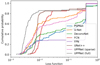 |
Fig. 2. Distribution of loss function values of neural networks randomly sampled from tested architectures trained in the task of pseudo-continuum prediction. One hundred random neural networks, with a number of trainable parameters ranging from 200 000 to 300 000, were drawn for each architecture. The training was held in a low-data regime for only 30 epochs. |
In the second step of exploration, the best neural network from each architecture was picked and trained in segmentation/pseudo-continuum prediction, and also in both tasks simultaneously. In the case of the simultaneous training, neural networks were equipped with two independent prediction heads. This training covered the entire synthetic dataset and lasted 150 epochs. The metrics were calculated on the same validation dataset as in the first step of exploration. The first 100 epochs used a learning rate equal to 10−4 and a learning rate equal to 10−5 was used for the remaining steps.
A brief summary of the results can be found in Table 1. Mean absolute error or accuracy is shown for each architecture and task. UPPNet (full), trained on both tasks simultaneously, is leading in pseudo-continuum prediction with MAE equal to 0.0110, while in segmentation the best is UPPNet (sparse), which is trained only in the segmentation task, with accuracy equal to 0.9166. The best, when trained in pseudo-continuum prediction only, is the U-Net network, with MAE equal to 0.0112. Training in both tasks simultaneously results in a systematic decrease in the segmentation quality but has little effect on the pseudo-continuum estimation. An overview of the original models used in the image semantic segmentation, with a short note about their one-dimensional versions, is provided below with the results and our conclusions.
Results of experiments with various neural network architectures on the validation dataset.
2.4.1. Fully convolutional network
This type of CNN was proposed by Long et al. (2015) and influenced the whole field of image semantic segmentation; most of the following architectures used in the semantic segmentation are also fully convolutional neural networks. This end-to-end trainable model uses a VGG-16 network (Simonyan & Zisserman 2015) as a backbone. This is a simple network that contains 16 trainable layers. The segmentation prediction is a function of feature maps previously upsampled by trained deconvolution layers from several intermediate representations, and merged by summation. This design gives spatial resolution and access to high-level semantic classes. In the context of one-dimensional spectrum processing, high-level semantic information can for example correspond to the presence of emission or wide absorption features in a spectrum. In all of the following networks, this is always the main goal: to somehow transfer to the final segmentation result the information about precise localisation that the input image contains, but also to discover the class of the complex objects present in the input. The schematic diagram of this architecture can be found in Fig. A.1.
Fully convolutional network architecture does not fit the comparison strategy used in our work, but we include it here as a prototype for all fully convolutional neural networks. It forms the low-resolution prediction, gradually refines it, and increases its resolution by upsampling and addition. This is contrary to other network architectures, which form high-resolution features used by a neural network head for the final prediction. Because of these characteristics, the FCN network that predicts pseudo-continuum and segmentation simultaneously was not implemented.
In the context of processing stellar spectra, this network has the poorest results among all tested architectures. The MAE of the predicted pseudo-continuum is equal to 0.0580 and the accuracy of segmentation is 0.8877. This shows that the strategy of upsampling a low-resolution prediction is not an efficient approach to the investigated problems.
2.4.2. Deconvolution network
This network (Noh et al. 2015) is an example of a so-called encoder-decoder architecture. It is composed of two parts: an encoder, the narrowing part, which is the VGG-16 network, and a decoder, the widening part, the mirrored VGG-16 where pooling is replaced with unpooling layers that use spatial positions of elements pooled in the decoder. This means that the localisation information is forwarded to the final segmentation output. The schematic diagram of this architecture can be found in Appendix A in Fig. A.2.
The one-dimensional version of this architecture gives moderate results (separate training: MAE = 0.0124, accuracy = 0.8991). Training in both tasks decreases prediction quality (C and S training: MAE = 0.0128, accuracy = 0.8763). To accurately preserve spatial location information, which is key to accurately predicting pseudo-continuum and segmentation, is the main challenge when using this architecture. We believe that this is the reason for the moderate performance of this network.
2.4.3. U-Net
The U-Net architecture proposed by Ronneberger et al. (2015) is a very successful and broadly exploited model. It is another encoder-decoder network. Its encoder is composed of five convolutional blocks that double the number of feature maps at each stage, and that are separated by a maximum pooling layer (comparison of pooling methods can be found in Scherer et al. 2010) a with 2 × 2 size and stride. The decoder is also composed of five blocks and upsamples the low-resolution, high semantic level feature maps, but contrary to the deconvolution network, blocks do not use only pooling indices but also concatenate the encoder feature map of the corresponding resolution. This is an example of the widely used concept of skipped connections, which helps to propagate the gradient in the training process, and helps the network to recover spatial localisation of objects in the input image. The blocks use 3 × 3 convolution kernels, except the final layer which uses 1 × 1 convolution for the final prediction. The schematic diagram of this architecture can be found in Fig. A.3.
Tested implementation of one-dimensional U-Net architecture gives very good results in both segmentation and pseudo-continuum prediction (separate training: MAE = 0.0112, accuracy = 0.9105). Its pseudo-continuum prediction MAE is the lowest among networks with one output. Simultaneous training to predict both targets does not lead to any improvement (C and S training: MAE = 0.0119, accuracy = 0.8866). This simple architecture is a very strong baseline for any further experiments.
2.4.4. UNet++
UNet++ (Zhou et al. 2018) is an extension of U-Net architecture. It replaces the skipped connections with densely connected blocks and uses deep supervision for regularisation. The authors of the original article introducing this architecture argue that the proposed connection scheme bridges a semantic gap between feature maps obtained in the encoder and decoder parts. The schematic diagram of this architecture can be found in Fig. A.4.
In the original work, the authors used intermediate supervision, but we do not use it for the sake of fair comparison to other architectures. Although, in theory, UNet++ is superior to the simpler U-Net architecture, the one-dimensional UNet++ network that we tested shows poor results (separate training: MAE = 0.0146, accuracy = 0.8945). Training in both tasks simultaneously slightly improves pseudo-continuum quality (MAE = 0.0133) but degrades segmentation substantially (accuracy = 0.8679). Nonetheless, we suspect that this architecture could outperform U-Net in the regime of bigger networks, where the U-Net performance could potentially saturate.
2.4.5. Feature pyramid network
The FPN was originally developed as a backbone for a two-stage object-detection model and was later used in a panoptic segmentation task (the task that unifies image semantic and instance segmentation; Kirillov et al. 2019). The basic idea is to incorporate the construction of a feature pyramid as a part of the neural network architecture. The feature pyramid is implemented as a path that upsamples the features using the nearest neighbour interpolation and uses lateral connections for better spatial localisation of high-resolution feature maps; it is visually similar to the U-Net architecture but conceptually implements a different idea. FPN propagates the same feature maps across different resolutions, while U-Net in principle may alter the feature maps towards the network output. The schematic diagram of this architecture can be found in Fig. A.5.
The FPN gives promising results in spectra processing (separate training: MAE = 0.0125, accuracy = 0.9063). Simultaneous task training (C and S) slightly improves the metrics of pseudo-continuum prediction (MAE = 0.0119) but worsens segmentation quality (accuracy = 0.8887).
2.4.6. Pyramid scene parsing network
The PSPNet (Zhao et al. 2017) is composed of three parts: a backbone network that delivers a feature map, a pyramid pooling module (PPM) that helps to introduce contextual information from different parts of an image to the final prediction, and an output convolutional network that is responsible for the final prediction. Use of the PPM is the novelty of PSPNet; PPM pools the features on different scales, applies 1 × 1 convolution and bilinear upsampling, and concatenates the produced features to input the feature map of the module. Zhao et al. (2017) show experimentally that such a lightweight module is able to introduce contextual information in the final prediction. The schematic diagram of this architecture can be found in Fig. A.6.
The one-dimensional version of PSPNet uses PPM depicted schematically in Fig. 3. Although PSPNet does not use skipped connections in between its encoder and decoder, it gives great results (separate training: MAE = 0.0115, accuracy = 0.9154). Its quality slightly degrades when trained on both tasks (C and S training: MAE = 0.0119, accuracy = 0.8914). Its results in pseudo-continuum prediction are very close to the results of U-Net, while in segmentation it achieves results that are about 0.5% better in accuracy.
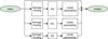 |
Fig. 3. Pyramid pooling module used in PSPNet and UPPNet networks. The PPM pools input feature maps at different scales, processes them using residual stages, linearly upsamples features to input resolution, and finally concatenates them with input features. In this work, the PPM pools the input features to all resolutions that strictly divide the input resolution, e.g. for feature resolutions equal to 32, it pools at scales of 2, 4, 8, and 16. The number of residual blocks in each RS and the number of features in each residual block were the same for all PPMs used in exploratory tests and were equal to 4 and 8, respectively. |
2.5. UPPNet
Insights from the previously mentioned architectures encouraged us to experiment with a different placement of skipped connections together with the use of PPMs. This led to U-Net with Pyramid Pooling Modules (UPPNet). First, we hypothesised that not all skipped connections are needed, but at the same time we suspected that PPMs included at some depths may result in better predictions. The proposed architecture is derived from U-Net by randomly dropping skipped connections or by replacing them with PPM. This version of UPPNet is denoted as sparse. U-Net, DeconvNet, and PSPNet are special cases of this architecture. Next, we decided to experiment with a version of UPPNet that is derived from the U-Net by replacing all skipped connections with PPMs, with an additional PPM module at the bottom of the network. This version of UPPNet is denoted as full. The schematic diagram of UPPNet (full) can be found in Fig. 4.
 |
Fig. 4. Diagram of U-Net with PPMs: UPPNet. The two RSs on the left create the narrowing path. The downward arrows represent strided residual blocks that decrease the sequence length by a factor of two. The central part has three PPM modules; the bottom one is preceded by a RS. The widening path on the right is a reflection of the narrowing path. Upward arrows represent upsampling by a factor of two. The upsampled features are concatenated with the result from the PPM blocks before being fed into the RS blocks. The depth of this UPPNet is defined as two. |
Figure 2 partially justifies the idea behind sparse UPPNet as there is a relatively large number of networks giving loss values lower that 4 × 10⁻³, but Table 1 shows that in the full training regime, this additional degree of freedom in skipped connection arrangement does not necessarily lead to better results than those obtained with U-Net and PSPNet (separate training: MAE = 0.0122, accuracy = 0.9166, C and S training: MAE = 0.0126, accuracy = 0.8857).
The regular UPPNet (full) architecture generally gives better results. Figure 2 shows that there are many models with a low loss value and that the best single network is of this kind. In the training on the full synthetic dataset (see Table 1), the advantage of this network decreases and the quality of pseudo-continuum prediction is comparable to that of U-Net and PSPNet models (separate training: MAE = 0.0116, C&S training: MAE = 0.0110). Nonetheless, the best result in pseudo-continuum normalisation belongs to UPPNet (full) architecture when trained in both tasks. Additionally, visual inspection of the results of U-Net and UPPNet showed that the latter gives slightly smaller residuals on hydrogen Hα and Hβ spectral lines which are important for atmospheric parameter estimation. The quality of segmentation is moderate in the case of training only in this task (accuracy = 0.9065), but is the best among models trained in both tasks simultaneously (accuracy = 0.9033). Because of these findings, the final model for pseudo-continuum prediction uses UPPNet (full) architecture as its main building block and is trained in both tasks simultaneously.
3. SUPP Network
Stacked U-Net with Pyramid Pooling Modules (SUPPNet) is a proposed neural network that gives the best results in the pseudo-continuum prediction task (see Table 1). This neural network was inspired by the three following well-known solutions present in machine learning literature: the U-Net architecture (Ronneberger et al. 2015), which, effective in tasks, is a basic block that combines precise localisation of features with complex semantic concepts, the pyramid scene parsing module (Zhao et al. 2017), which enables more effective sharing of contextual information across the whole receptive field, and the stacked hourglass network (Newell et al. 2016), where repetitive bottom-up processing in conjunction with deep supervision allows the network to learn fine-grained predictions.
3.1. Architecture details
SUPPNet is composed of two UPPNet (full) blocks and four prediction heads (Seg 1, Seg 2, Cont 1 and Cont 2; see Fig. 5). The UPPNet module was chosen as the main building block because of its high quality; reviewed in Sect. 2.5. The heads compute final predictions from the high-resolution feature maps created by UPPNet blocks and have simple architecture, which is described in Sect. 2.4. The first block is responsible for the coarse prediction of a continuum/non-continuum segmentation mask (Seg 1) and pseudo-continuum (Cont 1); these outputs are used only while training, for deep supervision (intermediate supervision) (Newell et al. 2016; Zhou et al. 2018), which is beneficial in two ways. First, it helps to deal with the vanishing gradient problem. Second, the deep supervision regularises the neural network model. As an input, the second block takes spectra, intermediate predictions (Seg 1 and Cont 1), and high-resolution feature maps from the first UPPNet block concatenated together. It outputs improved features that are used by the Seg 2 and Cont 2 heads for final predictions.
 |
Fig. 5. Block diagram of the proposed SUPP Network. The network is composed of two UPPNet blocks and four prediction heads. The first UPPNet block forms coarse predictions, and high-resolution feature maps that are forwarded to the second block (dashed arrow). The coarse predictions in intermediate outputs Cont 1 and Seg 1 (first pseudo-continuum and segmentation outputs, respectively) are forwarded to the second block. The second block forms the final predictions at Cont 2 and Seg 2 outputs. |
Both UPPNet blocks share hyper-parameters (e.g. a depth, a number of residual blocks in each residual stage (RS), etc.) but not their weights. The choice of hyper-parameters was based on a sampling of 400 UPPNet models that were trained in a low-data regime in a pseudo-continuum prediction task, following the procedure from Sect. 2.4. Subsequently, the best UPPNet was selected. The depth of this model is equal to 8 (its narrowing path has eight pooling layers in total), with the number of residual blocks in residual stages successively equal to 1, 1, 1, 2, 2, 5, 6, 7, 10, 7, 6, 5, 2, 2, 1, 1, and 1 with the number of filters at each stage equal to 12, 16, 16, 20, 24, 32, 44, 44, 44, 44, 44, 32, 24, 20, 16, 16, and 12, respectively. The narrowing and widening parts are symmetrical with the bottom residual stage. PPM modules in SUPPNet have four filters and use residual stages that are composed of a single residual block. Their group width is equal to 64, and so residual stages effectively use non-grouped convolutions. The total number of free parameters of the proposed SUPPNet is approximately equal to one million.
3.2. Training details
First, the SUPPNet model was trained on a synthetic dataset only. The training data were fed into the model using a data generator that augments training examples by randomly cropping the spectra with ratios ranging from 0.7 to 2.5, reflecting the spectrum over the y-axis with 0.5 probability, and adding Gaussian noise to obtain a S/N from 30 to 500. A ratio of one means that an input sampling of 0.03 Å was kept. A ratio of 0.7 corresponds to a sampling of 0.021 Å and a spectral range of 170 Å (170 ≈ 0.021 × 8192), and 2.5 to a sampling of 0.075 Å that corresponds to a 610 Å input window width. In this setting, the average sampling of the training data was equal to 0.05 Å and this is the value used later for prediction.
The Nadam optimiser was used for training as in all other experiments described in this work. The learning rate (lr) was equal to 10−4 for the first 100 epochs and was decreased to 10−5 for the remaining 50 epochs. After these 150 epochs, a learning curve flattened. We did not experiment with different parameters of the Nadam optimiser and left them equal to their default values (β1 = 0.9, β2 = 0.999). The batch size is 128. We denote this version SUPPNet (synth, S).
For active learning, the SUPPNet (synth) model was loaded and the learning continued for the next 100 epochs (for first 50 epochs lr = 10−4, and later lr = 10−5), using the same augmentations but with 10% of the synthetic training, examples replaced with spectra, and pseudo-continua acquired from manual normalisation. This resulted in the SUPPNet (active, A) network.
All neural network outputs were used in the training process. As in previous experiments, a mean squared error was used as a loss for pseudo-continuum regression, and mean binary cross-entropy for segmentation. The MSE loss was multiplied by a factor of 400 to give it the same order of magnitude as loss used in segmentation branches.
3.3. Spectrum processing
The proposed spectrum normalisation method consists of three stages. First, the spectrum is re-sampled with the sampling of 0.05 Å, and the sliding window of 8192 samples in size with a shift of 256 samples is applied. This particular shift means that each sample is normalised 8192/256 = 32 times. The data prepared in this way are then re-scaled (min-max normalisation is applied). The second step is the application of the SUPP Network. As the post-processing step, the predicted pseudo-continua are scaled back. Finally, the result is calculated as a weighted average over all predictions for each sample. This is also used to obtain a qualitative measure of the model’s inherent uncertainty of both predictions (pseudo-continuum and segmentation).
The processing described above gives final pseudo-continuum and segmentation mask predictions. Because of the noisy pattern of the order of 0.001 of the relative magnitude present in the final result, we recommend an application of additional final post-processing. We used a smoothing spline available in the SciPy Python module (Virtanen et al. 2020, function UnivariateSpline). A useful advantage of this approach to smoothing is the possibility to incorporate the estimated pseudo-continuum errors in the smoothing process. A smoothing spline fit contains a knot arrangement that takes into account the uncertainty of the predicted pseudo-continuum. For example, it places fewer knots in the ranges of greater uncertainty. An example SUPPNet result can be found in Fig. 1.
4. Results
Several statistics were used for SUPPNet normalisation quality assessment. All were computed using residuals between the normalised spectrum (manually or automatically using SUPPNet) and the reference normalised spectrum. Either the synthetic or manually normalised spectrum served as the reference spectrum. Observed spectra analysed here come from UVES POP, while synthetic spectra were computed using ATLAS/SYNTHE codes. Among all normalised UVES POP spectra, six were chosen as representative and were normalised by three of us (TR, EN, and NP). These spectra show most of the features present in stellar spectra (for a detailed description see the following text and Table 2). Statistics mostly used in this section are the following percentiles: 2.28, 15.87, 50.00 (median), 84.13, 97.73, and root-mean-square (RMS) error. In the case of normally distributed residuals, 15.87–84.13 and 2.28–97.73 ranges correspond to respectively one- and two-sigma bands.
Stars for the detailed normalisation quality assessment.
The significance of the obtained results was tested using the bootstrap method. We tested the hypothesis that median and measure of spread, defined as the difference between 15.87 and 84.13 residuals, are equal in tested groups. In all statements regarding significance, we adopted 95% symmetrical confidence intervals.
4.1. Synthetic spectra normalisation
To measure normalisation quality and minimise uncertainty introduced by the manual normalisation, the first test used only synthetic spectra. First of all, six chosen stars were modelled using ATLAS/SYNTHE codes. Parameters for synthetic spectra were taken from Table 2 and related articles. Missing parameters were manually estimated to be equal to Teff = 30 000 K and log g = 3.15 in the case of the star HD 155806 (O7.5 IIIe), and log g = 3.90 for HD 90882 (B9.5 V). The synthetic normalised spectrum for each star was then multiplied by about 200 different pseudo-continua derived from the manual normalisation. This gave about 1200 spectra in total, which were later normalised using the two versions of SUPPNet (synth and active), and used to calculate normalisation metrics.
The summary statistics of this experiment can be found in the top two rows of Table 3, and in Fig. 6 and Fig. B.1. The medians of the residuals, which measure a normalisation bias, are between −0.0016 (SUPPNet active, HD 25069, K0 III) and 0.0017 (SUPPNet synth, HD 27411, A3m). The residuals in the case of SUPPNet trained using active learning are systematically smaller than when trained using only the synthetic dataset. This means that the latter places pseudo-continuum systematically lower. The dispersion of residuals measured as a difference between 84.13 and 15.87 percentiles is between 0.0022 (SUPPNet synth, HD 155806, O7.5 IIIe) and 0.0095 (SUPPNet synth, HD 27411, A3m). The residuals are often slightly smaller when active learning is applied. For SUPPNet trained using the active learning, the dispersion of residuals is slightly but significantly smaller in the case of HD 27411 (A3m), HD 37495 (G4 V), and HD 25069 (K0 III), and is significantly larger for HD 90882 (B9.5 V). There are no statistically significant differences between dispersions of residuals for HD 155806 (O7.5 V) and HD 37495 (F4 V). The detailed inspection of Fig. 6 shows that systematic errors vary significantly across both wavelength and spectra parameters. They are especially prominent for A3m (HD 27411) and F4V (HD 37495) stars at wavelength shorter than 4500 Å, where they reach 0.03. Figure 7 shows a close-up of the 3900–4500 Å wavelength range of the A3 V synthetic spectra with the mean normalisation result and residuals. It can be seen that a significant normalisation bias arises in a range where the whole spectrum is below the continuum level. Leaving aside the regions described above, the average bias of normalization for synthetic spectra is typically below 0.01.
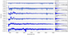 |
Fig. 6. Results of normalisation of six synthetic spectra multiplied by six manually fitted pseudo-continua trained with the application of active learning (synthetic data supplemented with manually normalised spectra). On the left of each row, we show the differences between automatically normalised spectra and synthetic spectra, and on the right we show the histograms of those differences with a related spectral type, median with 15.87 percentile in the upper index, and 84.13 percentile in the lower index. The dashed lines on each panel correspond to the residuals, which are equal to −0.01, 0.0, and 0.01, respectively. The use of active learning resulted in a slight reduction in the dispersion of residuals. |
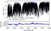 |
Fig. 7. Close-up of the 3900–4500 Å spectral range of the A3 V synthetic spectrum with a median of synthetic automatically normalised spectra (top panel) and residuals of normalisation errors (bottom panel). For this particular part of the spectrum, the average normalisation is significantly biased. These differences arise due to wide hydrogen absorption lines and strong metal lines which heavily blend in this spectral range. See Fig. 6 for the remaining results. |
Summary statistics of the detailed analysis of chosen representative stars and the normalisation of synthetic spectra.
We consider this statistics to be close to the realistic normalisation uncertainty in wavelength ranges with spectral features well represented in synthetic models. Nonetheless, normalisation of the synthetic spectra does not allow us to draw conclusions about the normalisation quality of the observed spectra, as they contain additional features (e.g. complex emission spectral lines).
4.2. Summary UVES POP normalisation statistics
Approximately 100 spectra from the UVES POP library were used to assess the quality of SUPPNet on observed stellar spectra. First, the majority of spectra from spectral type O to G were manually normalised. Spectra were then normalised using both versions of SUPPNet, and residuals’ statistics were calculated. The results are summarised in Fig. 8.
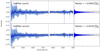 |
Fig. 8. Quality of normalisation measured using residuals between the result of the SUPPNet method and the manually normalised spectra over all stars from UVES POP field stars, which were manually normalised. The line shows the value of median for each wavelength, the shaded areas are defined to contain respectively 68 and 95 percent of values (defined by percentiles: 2.28, 15.87, 84.13, and 97.73). The upper and lower panels contain results of the algorithm that used only synthetic data for training or applied active learning, respectively. Active learning significantly reduces systematic effects for wavelengths shorter than 4500 Å. |
In the case of the model trained using only synthetic data, some biases are prominent around 6750 Å and for wavelengths shorter than 4500 Å. Strong telluric lines at approximately 6870 Å, which were absent in synthetic spectra, are the cause of the first bias. The second problem appears because SUPPNet (synth) systematically predicts an overly low pseudo-continuum in wide hydrogen absorption lines of A and F spectral types. Figures B.2–B.6 show separate plots for each spectral type. The median of residuals is significantly different from zero and is equal to −0.0006, which means that the model places pseudo-continua slightly above the levels chosen by astronomers. The dispersion of residuals measured as a difference between 84.13 and 15.87 percentiles is equal to 0.0124. Root mean squared error equals 0.0122.
SUPPNet trained using an active learning approach shows slightly better characteristics. The dispersion of its residuals (0.0118, RMS = 0.0128) is not significantly different from the SUPPNet (synth), but most of the systematic effects that can be seen in Fig. 8 are reduced (compare bias in wavelengths shorter than 4500 Å) after training that included real spectra. Nonetheless, SUPPNet (active) shares the tendency of the model trained on a synthetic dataset to place the pseudo-continuum higher than when a spectrum is manually normalised. This tendency is measured by a median of residuals equal to −0.0018 which is significantly (for a 95% confidence interval) different from zero. This effect can potentially be introduced by the human, who often models pseudo-continuum to lie lower than in reality. Differences between the medians of residuals for the two SUPPNet versions, although statistically significant, are at most comparable and often smaller than the intrinsic error of manual normalisation described in detail in Sect. 4.3.
Normalisation quality and active learning importance vary significantly across spectral types. In general, the later the spectral type, the larger the dispersion of normalisation residuals. Differences between the medians of the residuals of the two versions of SUPPNet for O, B, and A type stars are statistically significant. However, SUPPNet synth and active are not significantly different in terms of the dispersions of residuals and the remaining medians. The results are summarised in Table 4 and summary plots for each spectral type can be found in Figs. B.2–B.6. The tendency to place pseudo-continuum higher than during manual normalisation holds for most spectral types, with the notable exception of G type stars. Upon inspection, we noticed that in spectral ranges with substantial narrow absorption line blending, where the continuum is absent across wide parts of a spectrum, the model tends to place pseudo-continuum below the correct level. A simple workaround for this SUPPNet limitation is to reduce default sampling from 0.05 Å to 0.03–0.04 Å when working with spectral types later than G5.
Summary of SUPPNet normalisation quality over UVES POP field stars divided into spectral types.
The second issue is the relatively high uncertainty in the Hα Balmer line, which is especially prominent in the case of F and A type stars. Closer examination showed that this can be explained by erroneous manual normalisation. For this spectral range, the manual normalisation is impossible as a wavy pattern introduced by imperfections of an instrument pipeline crosses and changes this spectral feature significantly (see Fig. 9 for details).
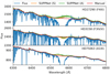 |
Fig. 9. Hα Balmer line region for the three UVES POP field stars. The figure shows how the wavy pattern prominent in pseudo-continua of F and A type stars is related to manual and SUPPNet predictions. The pseudo-continuum predicted by SUPPNet (A) is shown with an estimate of its uncertainty (method internal uncertainty, green shaded area). |
The positive influence of active learning on SUPPNet normalisation quality is the most prominent in the case of O type stars, where strong emission features are often present. The spectral range of HD 148937 (O6.5), with Hα Balmer and He I 6678 Å lines in emission, is shown in Fig. 10. SUPPNet (active) predicts pseudo-continuum across these features relatively well, while SUPPNet, trained using synthetic data only, treats these features as a part of the pseudo-continuum.
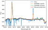 |
Fig. 10. Predicted pseudo-continuum for a spectrum of HD 148937 (O6.5) with Hα and HeI 6678 Å lines in emission. SUPPNet (active) correctly deals with most emission features, while SUPPNet (synth) treats those features as a part of pseudo-continuum. This is an important example of where active learning significantly improves the normalisation quality. |
4.3. Detailed analysis of chosen stars
In the last step of the SUPPNet analysis, six stars were normalised automatically and manually by three of us (TR, EN and NP), and the results were carefully compared. Their spectral types range from O7.5 V to K0 III and show most of the typical spectral features. The main characteristics of the selected stars are gathered in Table 2.
HD 155806 (HR 6397, V = 5.53 mag) is the hottest Galactic Oe star (Fullerton et al. 2011). Its initial spectral classification of O7.5 V[n]e (Walborn 1973) was changed to O7.5 IIIe because of the strength of its metallic features (Negueruela et al. 2004). Stars of this type are rare and show a double-peaked or central emission in their Balmer lines.
HD 27411 (HR 1353, V = 6.06 mag, A3m) is an example of a chemically peculiar (CP) star. Its atmospheric parameters and abundances were investigated in detail in the context of diffusion theory in the work of Catanzaro & Balona (2012).
HD 90882 (HR 4116, δ Sex, B9.5 V), HD 37495 (HR 1935, ν2 Col, F5 V), and HD 59967 (HR 2882, G3 V) are typical representatives of their spectral types. The first is a rapidly rotating B type star, and the last is a young (≈0.4 Gyr), active, slowly rotating solar-twin star.
The last star for detailed analysis is HD 25069 (HR 1232, V = 5.83 mag). In the UVES POP catalogue, its spectral type is G9 V, while SIMBAD database sources give K0 III or K0/1 III. Here K0 III is used. This star is a representative example of a late G and early K spectral type.
The results for all stars can be found in the four bottom rows of Table 3. Figure 11 contains detailed pseudo-continua and residuals for the HD 27411 (A3m) star. The results show that the differences between manually normalised spectra are between −0.0042 and 0.0016 in the median with typical dispersion, defined by a 15.87–84.13 percentiles band ranging from approximately 0.0040 to 0.0330 (see NP–TR and EN–TR rows in Table 3). This is the scale of uncertainty inherent to manual normalisation. In terms of residuals statistics, the quality of the SUPPNet normalisation method is superior to the quality of the manual normalisation.
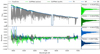 |
Fig. 11. Comparison of normalisation quality using the example of HD 27411 (A3m) with two versions of the proposed method (SUPPNet active and synth) and manual normalisation performed independently by three different people (TR, NP, and EN). Upper left panel: original flux with all fitted pseudo-continua. Lower left panel: residuals of normalised fluxes relative to TR normalisation. Right panels: present histograms of all mentioned residuals with median, 15.87, and 84.13 percentiles. |
The left panels of Fig. 11 and Figs. B.7–B.11 demonstrate the difficulty of the task of fitting a pseudo-continuum. In HD 27411, most of the spectrum is disturbed by a semi-periodic pattern that arises from imperfect order merging and blaze function removal. SUPPNet models this pseudo-continuum type relatively well for wavelengths longer than the Balmer Hβ line and significantly poorer in the spectral range from 4400 to 4800 Å, where the amplitude and frequency of this pattern significantly increase. Nonetheless, the error amplitude is of the order of 0.02, both for manual and SUPPNet normalisation. For wavelengths shorter than 4200 Å, the dispersion between different normalised fluxes grows considerably. In this range, it is difficult to assess the normalisation quality without referring to the synthetic spectral model, which could potentially guide manual normalisation.
The uncertainty estimated by SUPPNets has only a qualitative meaning, and informs the users of where they can expect normalisation results to be most uncertain, but not necessarily where the model failed in predicting the pseudo-continuum. As can be seen in the bottom panel of Fig. 11, the estimated uncertainty is the highest in the wide absorption lines. However, in the spectral range from 4400 to 4800 Å, the proposed method did not capture the ambiguous character of the predicted pseudo-continuum.
4.4. Resolution, rotational velocity, and noise
Stellar spectra present in databases have various levels of noise, resolutions, and projected rotational velocities. We tested the consistency of normalisation with respect to those parameters. To this end, we used synthetic spectra calculated for parameters of HD 27411 (A3m) with a S/N of 30 and 500, a projected rotational velocity equal to 0, 50, 100, and 200 km s−1, and resolutions equal to 104 and 105.
The predicted pseudo-continuum is generally consistent for the tested S/Ns. The differences between results increase for low-resolution spectra and in heavily blended line regions where there is no real continuum in the flux. The test with low-quality medium-resolution spectra showed that in this case, the proposed method places the pseudo-continuum significantly too high. This problem can be suppressed by increasing a sampling step or by training SUPPNet using noisy, low-resolution spectra.
For a spectrum broadened by the projected rotational velocity, the differences between predicted pseudo-continua are generally smaller than 0.01, except for the wavelengths shorter than 4300 Å where the flux is well below expected pseudo-continuum. The results described above are summarised in Fig. C.1.
5. Conclusions
Machine learning methods are becoming more and more important in science, particularly in astronomy. Here we present a method for spectrum normalisation that uses novel, one-dimensional, fully convolutional, deep neural network architecture: the SUPP Network. Its automatic character makes the results of SUPPNet reproducible and more homogeneous, which is very important especially in the context of time-series of spectra. The use of synthetic spectra during training allows the model to become aware of features present in the spectra and helps to recover pseudo-continuum in regions where this cannot be done manually; for example, in regions heavily blended by lines or across Balmer hydrogen lines with instrumental ripples. The accuracy of SUPPNet is comparable to that achieved with careful manual normalisation, making it possible to omit human intervention in this step of spectrum pre-processing. SUPPNet works well with both emission and absorption spectral features, with blended lines and spectral ranges where the real continuum is absent. If manual correction is necessary, it can be done using a developed Python application or online; see Appendix D.
The main drawback of the proposed method is the fact that it uses a sliding window technique while in principle this is not necessary for fully convolutional neural networks, as they accept inputs of any length. Sliding window is necessary because we use a min-max normalisation strategy for inputs. As a beneficial side effect, we are able to give some estimates of pseudo-continuum uncertainty.
The directions of future developments are as follows: extension of the training set to include spectra from spectrographs other than UVES and FEROS, an extension of the set of empirical pseudo-continua to include fits from other astronomers, experiments with alternative input normalisation techniques that would eliminate the sliding window approach, and exploration of alternative ways to estimate prediction uncertainties. pseudo-continua provided by other astronomers and observations from different instruments are expected to reduce biases. The proposed technique can be extended in such a way that it uses coarse spectral type estimation and wavelength range information, which can further improve normalisation quality. Other possible development paths are exploitation of different neural network architectures and modules (e.g. attention module) and scaling-up of the SUPPNet model. The longstanding purpose is to use an automatically normalised spectrum for stellar parameter and abundance estimation that consistently includes normalisation errors.
The most important characteristic of the proposed method is its generality. The use of SUPPNet in similar tasks is straightforward, such as in trend or background modelling, and UPP modules can be used in contexts other than those related to one-dimensional signal processing; for example image segmentation.
Acknowledgments
T. Różański was financed from budgetary funds for science in 2018-2022 as a research project under the program “Diamentowy Grant”, no. DI2018 024648. Research project partly supported by program “Excellence initiative – research university” for years 2020–2026 for University of Wrocław.
References
- Abadi, M., Agarwal, A., Barham, P., et al. 2015, TensorFlow: Large-Scale Machine Learning on Heterogeneous Systems, Software available from tensorflow.org [Google Scholar]
- Aguilera-Gómez, C., Ramírez, I., & Chanamé, J. 2018, A&A, 614, A55 [NASA ADS] [CrossRef] [EDP Sciences] [Google Scholar]
- Antoniadis-Karnavas, A., Sousa, S. G., Delgado-Mena, E., et al. 2020, A&A, 636, A9 [NASA ADS] [CrossRef] [EDP Sciences] [Google Scholar]
- Bagnulo, S., Jehin, E., Ledoux, C., et al. 2003, Messenger, 114, 10 [NASA ADS] [Google Scholar]
- Ball, N. M., & Brunner, R. J. 2010, Int. J. Modern Phys. D, 19, 1049 [NASA ADS] [CrossRef] [Google Scholar]
- Baron, D. 2019, Machine Learning in Astronomy: a Practical Overview [arXiv:1904.07248] [Google Scholar]
- Cadusch, P. J., Hlaing, M. M., Wade, S. A., McArthur, S. L., & Stoddart, P. R. 2013, J. Raman Spectr., 44, 1587 [NASA ADS] [CrossRef] [Google Scholar]
- Carleo, G., Cirac, I., Cranmer, K., et al. 2019, Rev. Mod. Phys., 91, 041001 [NASA ADS] [CrossRef] [Google Scholar]
- Catanzaro, G., & Balona, L. A. 2012, MNRAS, 421, 1222 [NASA ADS] [CrossRef] [Google Scholar]
- Cretignier, M., Francfort, J., Dumusque, X., Allart, R., & Pepe, F. 2020, A&A, 640, A42 [NASA ADS] [CrossRef] [EDP Sciences] [Google Scholar]
- dos Santos, L. A., Meléndez, J., do Nascimento, J. D., et al. 2016, A&A, 592, A156 [NASA ADS] [CrossRef] [EDP Sciences] [Google Scholar]
- Dozat, T. 2016, Incorporating Nesterov Momentum into Adam [Google Scholar]
- Farias, H., Ortiz, D., Damke, G., Jaque Arancibia, M., & Solar, M. 2020, Astron. Comput., 33, 100420 [NASA ADS] [CrossRef] [Google Scholar]
- Fullerton, A. W., Petit, V., Bagnulo, S., & Wade, G. A. 2011, in Active OB Stars: Structure, Evolution, Mass Loss, and Critical Limits, eds. C. Neiner, G. Wade, G. Meynet, & G. Peters, 272, 182 [NASA ADS] [Google Scholar]
- Gaia Collaboration (Prusti, T., et al.) 2016, A&A, 595, A1 [NASA ADS] [CrossRef] [EDP Sciences] [Google Scholar]
- George, D., & Huerta, E. 2018, Phys. Lett. B, 778, 64 [NASA ADS] [CrossRef] [Google Scholar]
- Hendriks, L., & Aerts, C. 2019, PASP, 131, 108001 [Google Scholar]
- Hoeser, T., & Kuenzer, C. 2020, Remote Sens., 12, 1667 [NASA ADS] [CrossRef] [Google Scholar]
- Hojjatpanah, S., Figueira, P., Santos, N. C., et al. 2019, A&A, 629, A80 [NASA ADS] [CrossRef] [EDP Sciences] [Google Scholar]
- Howarth, I. D., Siebert, K. W., Hussain, G. A. J., & Prinja, R. K. 1997, MNRAS, 284, 265 [NASA ADS] [CrossRef] [Google Scholar]
- Ivezić, V., Kahn, S. M., Tyson, J. A., et al. 2019, ApJ, 873, 111 [NASA ADS] [CrossRef] [Google Scholar]
- Kingma, D. P., & Ba, J. 2017, Adam: A Method for Stochastic Optimization [arXiv:1412.6980] [Google Scholar]
- Kirillov, A., Girshick, R., He, K., & Dollár, P. 2019, Panoptic Feature Pyramid Networks [arXiv:1901.02446] [Google Scholar]
- Kukačka, J., Golkov, V., & Cremers, D. 2017, ArXiv e-prints [arXiv:1710.10686] [Google Scholar]
- Kurucz, R. L. 1970, SAO Special report, 309 [Google Scholar]
- Lanz, T., & Hubeny, I. 2003, ApJS, 146, 417 [NASA ADS] [CrossRef] [Google Scholar]
- Lanz, T., & Hubeny, I. 2007, ApJS, 169, 83 [CrossRef] [Google Scholar]
- LeCun, Y., Boser, B., Denker, J. S., et al. 1989, Neural Comput., 1, 541 [NASA ADS] [CrossRef] [Google Scholar]
- Lin, T. Y., Dollár, P., Girshick, R., et al. 2017, Feature Pyramid Networks for Object Detection [arXiv:1612.03144] [Google Scholar]
- Long, J., Shelhamer, E., & Darrell, T. 2015, Fully Convolutional Networks for Semantic Segmentation [arXiv:1411.4038] [Google Scholar]
- Mahabal, A., Rebbapragada, U., Walters, R., et al. 2019, PASP, 131, 038002 [NASA ADS] [CrossRef] [Google Scholar]
- Majewski, S. R., Schiavon, R. P., Frinchaboy, P. M., et al. 2017, AJ, 154, 94 [NASA ADS] [CrossRef] [Google Scholar]
- Negueruela, I., Steele, I. A., & Bernabeu, G. 2004, Astron. Nachr., 325, 749 [Google Scholar]
- Nesterov, Y. E. 1983, Dokl. akad. nauk Sssr, 269, 543 [Google Scholar]
- Newell, A., Yang, K., & Deng, J. 2016, Stacked Hourglass Networks for Human Pose Estimation [arXiv:1603.06937] [Google Scholar]
- Nissen, P. E., Christensen-Dalsgaard, J., Mosumgaard, J. R., et al. 2020, A&A, 640, A81 [NASA ADS] [CrossRef] [EDP Sciences] [Google Scholar]
- Noh, H., Hong, S., & Han, B. 2015, Learning Deconvolution Network for Semantic Segmentation [arXiv:1505.04366] [Google Scholar]
- Radosavovic, I., Prateek Kosaraju, R., Girshick, R., He, K., & Dollár, P. 2020, ArXiv e-prints [arXiv:2003.13678] [Google Scholar]
- Ronneberger, O., Fischer, P., & Brox, T. 2015, U-Net: Convolutional Networks for Biomedical Image Segmentation [arXiv:1505.04597] [Google Scholar]
- Royer, F. 2009, On the Rotation of A-Type Stars, 765, 207 [NASA ADS] [CrossRef] [Google Scholar]
- Savitzky, A., & Golay, M. J. E. 1964, Anal. Chem., 36, 1627 [Google Scholar]
- Scherer, D., Müller, A., & Behnke, S. 2010, in International Conference on Artificial Neural Networks (Springer), 92 [Google Scholar]
- Schröder, C., Reiners, A., & Schmitt, J. H. M. M. 2009, A&A, 493, 1099 [NASA ADS] [CrossRef] [EDP Sciences] [Google Scholar]
- Simonyan, K., & Zisserman, A. 2015, Very Deep Convolutional Networks for Large-Scale Image Recognition [arXiv:1409.1556] [Google Scholar]
- Swihart, S. J., Garcia, E. V., Stassun, K. G., et al. 2017, AJ, 153, 16 [Google Scholar]
- Virtanen, P., Gommers, R., Oliphant, T. E., et al. 2020, Nat. Methods, 17, 261 [Google Scholar]
- Škoda, P., Podsztavek, O., & Tvrdík, P. 2020, A&A, 643, A122 [NASA ADS] [CrossRef] [EDP Sciences] [Google Scholar]
- Walborn, N. R. 1973, AJ, 78, 1067 [NASA ADS] [CrossRef] [Google Scholar]
- Xie, S., Girshick, R., Dollár, P., Tu, Z., & He, K. 2016, ArXiv e-prints [arXiv:1611.05431] [Google Scholar]
- Xu, X., Cisewski-Kehe, J., Davis, A. B., Fischer, D. A., & Brewer, J. M. 2019, AJ, 157, 243 [NASA ADS] [CrossRef] [Google Scholar]
- Zhao, G., Zhao, Y., Chu, Y., Jing, Y., & Deng, L. 2012, LAMOST Spectral Survey [arXiv:1206.3569] [Google Scholar]
- Zhao, H., Shi, J., Qi, X., Wang, X., & Jia, J. 2017, Pyramid Scene Parsing Network [arXiv:1612.01105] [Google Scholar]
- Zhou, Z., Siddiquee, M. M. R., Tajbakhsh, N., & Liang, J. 2018, UNet++: A Nested U-Net Architecture for Medical Image Segmentation [arXiv:1807.10165] [Google Scholar]
- Zorec, J., & Royer, F. 2012, A&A, 537, A120 [NASA ADS] [CrossRef] [EDP Sciences] [Google Scholar]
Appendix A: Diagrams of neural network architectures
Block diagrams of neural network architectures included in exploratory tests.
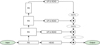 |
Fig. A.1. Fully convolutional network (FCN; Long et al. 2015) |
 |
Fig. A.2. Deconvolution network (DeconvNet Noh et al. 2015) |
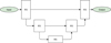 |
Fig. A.3. U-Net (Ronneberger et al. 2015) |
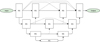 |
Fig. A.4. UNet++ (Zhou et al. 2018) |
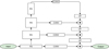 |
Fig. A.5. Feature pyramid network (FPN, Lin et al. 2017; Kirillov et al. 2019) |
 |
Fig. A.6. Pyramid scene parsing network (PSPNet, Zhao et al. 2017) |
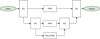 |
Fig. A.7. U-Net with pyramid pooling module (UPPNet, this work) |
Appendix B: Plots
Detailed plots of the results.
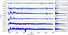 |
Fig. B.1. Results of normalisation of six synthetic spectra multiplied by six manually fitted pseudo-continua using a neural network trained only with synthetic data. In each row, on the left, the differences between automatically normalised spectra and synthetic spectrum are shown, and on the right, the histogram of those differences with a related spectral type, the median with 15.87 percentile in the upper index, and 84.13 percentile in the lower index is displayed. The dashed lines on each panel correspond to the residuals equal to -0.01, 0.0, and 0.01, respectively. |
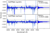 |
Fig. B.2. Residuals between the manually normalised spectrum and the result of the tested algorithm over O type stars from UVES POP field stars, which were manually normalised. |
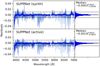 |
Fig. B.3. Residuals between the manually normalised spectrum and the result of the tested algorithm over B type stars from UVES POP field stars, which were manually normalised. |
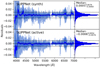 |
Fig. B.4. Residuals between the manually normalised spectrum and the result of the tested algorithm over A type stars from UVES POP field stars, which were manually normalised. |
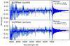 |
Fig. B.5. Residuals between the manually normalised spectrum and the result of the tested algorithm over F type stars from UVES POP field stars, which were manually normalised. |
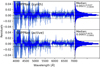 |
Fig. B.6. Residuals between the manually normalised spectrum and the result of the tested algorithm over G type stars from UVES POP field stars, which were manually normalised. |
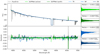 |
Fig. B.7. Comparison of normalisation quality on the example of HD 155806 (O7.5 V) star with two versions of the proposed method (SUPPNet active and synth) and manual normalisation done independently by three different people (TR, NP, and EN). The left upper panel shows original flux with all fitted pseudo-continua. The left lower panel shows residuals of normalised fluxes relative to TR normalisation. The right panel presents histograms of all mentioned residuals with median, 15.87, and 84.13 percentiles. |
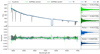 |
Fig. B.8. Comparison of normalisation quality on the example of HD 90882 (B9.5 V) star with two versions of the proposed method (SUPPNet active and synth) and manual normalisation done independently by three different people (TR, NP, and EN). The left upper panel shows original flux with all fitted pseudo-continua. The left lower panel shows residuals of normalised fluxes relative to TR normalisation. The right panel presents histograms of all mentioned residuals with median, 15.87, and 84.13 percentiles. |
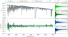 |
Fig. B.9. Comparison of normalisation quality on the example of HD 37495 (F4 V) star with two versions of the proposed method (SUPPNet active and synth) and manual normalisation done independently by three different people (TR, NP, and EN). The left upper panel shows original flux with all fitted pseudo-continua. The left lower panel shows residuals of normalised fluxes relative to TR normalisation. The right panel presents histograms of all mentioned residuals with median, 15.87, and 84.13 percentiles. |
 |
Fig. B.10. Comparison of normalisation quality on the example of HD 59967 (G4 V) star with two versions of the proposed method (SUPPNet active and synth) and manual normalisation done independently by three different people (TR, NP, and EN). The left upper panel shows original flux with all fitted pseudo-continua. The left lower panel shows residuals of normalised fluxes relative to TR normalisation. The right panel presents histograms of all mentioned residuals with median, 15.87, and 84.13 percentiles. |
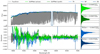 |
Fig. B.11. Comparison of normalisation quality on the example of HD 25069 (K0 III) star with two versions of the proposed method (SUPPNet active and synth) and manual normalisation done independently by three different people (TR, NP, and EN). The left upper panel shows original flux with all fitted pseudo-continua. The left lower panel shows residuals of normalised fluxes relative to TR normalisation. The right panel presents histograms of all mentioned residuals with median, 15.87, and 84.13 percentiles. |
Appendix C: Resolution, rotational velocity, and noise
The results of resolution, rotation velocity, and noise influence on predicted pseudo-continuum are summarised in Fig. C.1
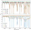 |
Fig. C.1. Normalised spectrum and pseudo-continuum predicted by SUPPNet (active) with default sampling and smoothing parameters. As flux is already normalised, pseudo-continuum should equal 1 in the whole domain. The upper panel shows the influence of noise and resolution on normalisation results. The results are generally consistent with the exception of noisy, SNR = 30, medium resolution, R = 104, spectra (see the green lines). In such a case the pseudo-continuum is placed too high. It is worth mentioning that such low resolution is outside of the training data domain where the resolution is not lower than 4 × 10⁴. This limitation can be overcome by increasing a sampling step or by extending the training set to include lower resolution spectra. The lower panel shows the influence of the projected rotational velocity on the normalisation result. The predictions are generally consistent and differ by less than 0.01. |
Appendix D: Codes
D.1. SUPPNet – online
An online version of the SUPPNet method is available: https://git.io/JqJhf. It is a fully front-end JavaScript application that gives access to the basic features of SUPPNet. It is a simple way to experiment with the proposed method and is intended to be the first choice for users who do not need all features of the full version of the code and for whom the performance offered by the website is sufficient. Additionally, the webpage contains interactive versions of plots gathered in this work.
Its basic limitations are a predetermined value of the sliding window shifts (equals 1024 samples), and a missing feature of adaptive spline smoothing which is replaced with Savicky-Golay filtering (Savitzky & Golay 1964) in the online version. Users interested in automatised normalisation of large sets of spectra are encouraged to use the Python version of the code.
D.2. SUPPNet – Python version
The Python version of SUPPNet includes all features for spectrum normalisation, with relatively easy access to GPU acceleration for users who need top performance. It is available on GitHub https://github.com/RozanskiT/suppnet.
D.3. HANDY
HANDY5 is an interactive tool for manual spectrum normalisation. pseudo-continuum fitting in HANDY is based on manual selection of parts of the continuum, to which the Chebyshev polynomial of the selected order is then fitted in the defined areas. Akima spline functions are used between these areas. Additionally, HANDY includes the possibility to interpolate spectrum on the predefined grid of synthetic spectra, wraps SYNTHE/ATLAS codes (Kurucz 1970), for spectrum synthesis that gives access to lines identification lists and includes radial velocity correction unit. The mentioned features make it a handy tool for initial spectrum exploration and/or manual normalisation.
All Tables
Results of experiments with various neural network architectures on the validation dataset.
Summary statistics of the detailed analysis of chosen representative stars and the normalisation of synthetic spectra.
Summary of SUPPNet normalisation quality over UVES POP field stars divided into spectral types.
All Figures
|
Fig. 1. Result of HD 27411 (A3m) spectrum processing. Left upper panel: the spectrum and the predicted continuum near the Hα line. Lower left panel: the corresponding segmentation mask. The shaded area denotes the estimated uncertainty. |
| In the text | |
|
Fig. 2. Distribution of loss function values of neural networks randomly sampled from tested architectures trained in the task of pseudo-continuum prediction. One hundred random neural networks, with a number of trainable parameters ranging from 200 000 to 300 000, were drawn for each architecture. The training was held in a low-data regime for only 30 epochs. |
| In the text | |
|
Fig. 3. Pyramid pooling module used in PSPNet and UPPNet networks. The PPM pools input feature maps at different scales, processes them using residual stages, linearly upsamples features to input resolution, and finally concatenates them with input features. In this work, the PPM pools the input features to all resolutions that strictly divide the input resolution, e.g. for feature resolutions equal to 32, it pools at scales of 2, 4, 8, and 16. The number of residual blocks in each RS and the number of features in each residual block were the same for all PPMs used in exploratory tests and were equal to 4 and 8, respectively. |
| In the text | |
|
Fig. 4. Diagram of U-Net with PPMs: UPPNet. The two RSs on the left create the narrowing path. The downward arrows represent strided residual blocks that decrease the sequence length by a factor of two. The central part has three PPM modules; the bottom one is preceded by a RS. The widening path on the right is a reflection of the narrowing path. Upward arrows represent upsampling by a factor of two. The upsampled features are concatenated with the result from the PPM blocks before being fed into the RS blocks. The depth of this UPPNet is defined as two. |
| In the text | |
|
Fig. 5. Block diagram of the proposed SUPP Network. The network is composed of two UPPNet blocks and four prediction heads. The first UPPNet block forms coarse predictions, and high-resolution feature maps that are forwarded to the second block (dashed arrow). The coarse predictions in intermediate outputs Cont 1 and Seg 1 (first pseudo-continuum and segmentation outputs, respectively) are forwarded to the second block. The second block forms the final predictions at Cont 2 and Seg 2 outputs. |
| In the text | |
|
Fig. 6. Results of normalisation of six synthetic spectra multiplied by six manually fitted pseudo-continua trained with the application of active learning (synthetic data supplemented with manually normalised spectra). On the left of each row, we show the differences between automatically normalised spectra and synthetic spectra, and on the right we show the histograms of those differences with a related spectral type, median with 15.87 percentile in the upper index, and 84.13 percentile in the lower index. The dashed lines on each panel correspond to the residuals, which are equal to −0.01, 0.0, and 0.01, respectively. The use of active learning resulted in a slight reduction in the dispersion of residuals. |
| In the text | |
|
Fig. 7. Close-up of the 3900–4500 Å spectral range of the A3 V synthetic spectrum with a median of synthetic automatically normalised spectra (top panel) and residuals of normalisation errors (bottom panel). For this particular part of the spectrum, the average normalisation is significantly biased. These differences arise due to wide hydrogen absorption lines and strong metal lines which heavily blend in this spectral range. See Fig. 6 for the remaining results. |
| In the text | |
|
Fig. 8. Quality of normalisation measured using residuals between the result of the SUPPNet method and the manually normalised spectra over all stars from UVES POP field stars, which were manually normalised. The line shows the value of median for each wavelength, the shaded areas are defined to contain respectively 68 and 95 percent of values (defined by percentiles: 2.28, 15.87, 84.13, and 97.73). The upper and lower panels contain results of the algorithm that used only synthetic data for training or applied active learning, respectively. Active learning significantly reduces systematic effects for wavelengths shorter than 4500 Å. |
| In the text | |
|
Fig. 9. Hα Balmer line region for the three UVES POP field stars. The figure shows how the wavy pattern prominent in pseudo-continua of F and A type stars is related to manual and SUPPNet predictions. The pseudo-continuum predicted by SUPPNet (A) is shown with an estimate of its uncertainty (method internal uncertainty, green shaded area). |
| In the text | |
|
Fig. 10. Predicted pseudo-continuum for a spectrum of HD 148937 (O6.5) with Hα and HeI 6678 Å lines in emission. SUPPNet (active) correctly deals with most emission features, while SUPPNet (synth) treats those features as a part of pseudo-continuum. This is an important example of where active learning significantly improves the normalisation quality. |
| In the text | |
|
Fig. 11. Comparison of normalisation quality using the example of HD 27411 (A3m) with two versions of the proposed method (SUPPNet active and synth) and manual normalisation performed independently by three different people (TR, NP, and EN). Upper left panel: original flux with all fitted pseudo-continua. Lower left panel: residuals of normalised fluxes relative to TR normalisation. Right panels: present histograms of all mentioned residuals with median, 15.87, and 84.13 percentiles. |
| In the text | |
|
Fig. A.1. Fully convolutional network (FCN; Long et al. 2015) |
| In the text | |
|
Fig. A.2. Deconvolution network (DeconvNet Noh et al. 2015) |
| In the text | |
|
Fig. A.4. UNet++ (Zhou et al. 2018) |
| In the text | |
|
Fig. A.5. Feature pyramid network (FPN, Lin et al. 2017; Kirillov et al. 2019) |
| In the text | |
|
Fig. A.6. Pyramid scene parsing network (PSPNet, Zhao et al. 2017) |
| In the text | |
|
Fig. A.7. U-Net with pyramid pooling module (UPPNet, this work) |
| In the text | |
|
Fig. B.1. Results of normalisation of six synthetic spectra multiplied by six manually fitted pseudo-continua using a neural network trained only with synthetic data. In each row, on the left, the differences between automatically normalised spectra and synthetic spectrum are shown, and on the right, the histogram of those differences with a related spectral type, the median with 15.87 percentile in the upper index, and 84.13 percentile in the lower index is displayed. The dashed lines on each panel correspond to the residuals equal to -0.01, 0.0, and 0.01, respectively. |
| In the text | |
|
Fig. B.2. Residuals between the manually normalised spectrum and the result of the tested algorithm over O type stars from UVES POP field stars, which were manually normalised. |
| In the text | |
|
Fig. B.3. Residuals between the manually normalised spectrum and the result of the tested algorithm over B type stars from UVES POP field stars, which were manually normalised. |
| In the text | |
|
Fig. B.4. Residuals between the manually normalised spectrum and the result of the tested algorithm over A type stars from UVES POP field stars, which were manually normalised. |
| In the text | |
|
Fig. B.5. Residuals between the manually normalised spectrum and the result of the tested algorithm over F type stars from UVES POP field stars, which were manually normalised. |
| In the text | |
|
Fig. B.6. Residuals between the manually normalised spectrum and the result of the tested algorithm over G type stars from UVES POP field stars, which were manually normalised. |
| In the text | |
|
Fig. B.7. Comparison of normalisation quality on the example of HD 155806 (O7.5 V) star with two versions of the proposed method (SUPPNet active and synth) and manual normalisation done independently by three different people (TR, NP, and EN). The left upper panel shows original flux with all fitted pseudo-continua. The left lower panel shows residuals of normalised fluxes relative to TR normalisation. The right panel presents histograms of all mentioned residuals with median, 15.87, and 84.13 percentiles. |
| In the text | |
|
Fig. B.8. Comparison of normalisation quality on the example of HD 90882 (B9.5 V) star with two versions of the proposed method (SUPPNet active and synth) and manual normalisation done independently by three different people (TR, NP, and EN). The left upper panel shows original flux with all fitted pseudo-continua. The left lower panel shows residuals of normalised fluxes relative to TR normalisation. The right panel presents histograms of all mentioned residuals with median, 15.87, and 84.13 percentiles. |
| In the text | |
|
Fig. B.9. Comparison of normalisation quality on the example of HD 37495 (F4 V) star with two versions of the proposed method (SUPPNet active and synth) and manual normalisation done independently by three different people (TR, NP, and EN). The left upper panel shows original flux with all fitted pseudo-continua. The left lower panel shows residuals of normalised fluxes relative to TR normalisation. The right panel presents histograms of all mentioned residuals with median, 15.87, and 84.13 percentiles. |
| In the text | |
|
Fig. B.10. Comparison of normalisation quality on the example of HD 59967 (G4 V) star with two versions of the proposed method (SUPPNet active and synth) and manual normalisation done independently by three different people (TR, NP, and EN). The left upper panel shows original flux with all fitted pseudo-continua. The left lower panel shows residuals of normalised fluxes relative to TR normalisation. The right panel presents histograms of all mentioned residuals with median, 15.87, and 84.13 percentiles. |
| In the text | |
|
Fig. B.11. Comparison of normalisation quality on the example of HD 25069 (K0 III) star with two versions of the proposed method (SUPPNet active and synth) and manual normalisation done independently by three different people (TR, NP, and EN). The left upper panel shows original flux with all fitted pseudo-continua. The left lower panel shows residuals of normalised fluxes relative to TR normalisation. The right panel presents histograms of all mentioned residuals with median, 15.87, and 84.13 percentiles. |
| In the text | |
|
Fig. C.1. Normalised spectrum and pseudo-continuum predicted by SUPPNet (active) with default sampling and smoothing parameters. As flux is already normalised, pseudo-continuum should equal 1 in the whole domain. The upper panel shows the influence of noise and resolution on normalisation results. The results are generally consistent with the exception of noisy, SNR = 30, medium resolution, R = 104, spectra (see the green lines). In such a case the pseudo-continuum is placed too high. It is worth mentioning that such low resolution is outside of the training data domain where the resolution is not lower than 4 × 10⁴. This limitation can be overcome by increasing a sampling step or by extending the training set to include lower resolution spectra. The lower panel shows the influence of the projected rotational velocity on the normalisation result. The predictions are generally consistent and differ by less than 0.01. |
| In the text | |
Current usage metrics show cumulative count of Article Views (full-text article views including HTML views, PDF and ePub downloads, according to the available data) and Abstracts Views on Vision4Press platform.
Data correspond to usage on the plateform after 2015. The current usage metrics is available 48-96 hours after online publication and is updated daily on week days.
Initial download of the metrics may take a while.